Second-principles method including electron and lattice degrees of freedom

Abstract

We present a first-principles-based (second-principles) scheme that permits large-scale materials simulations including both atomic and electronic degrees of freedom on the same footing. The method is based on a predictive quantum-mechanical theory – e.g., Density Functional Theory – and its accuracy can be systematically improved at a very modest computational cost. Our approach is based on dividing the electron density of the system into a reference part – typically corresponding to the system’s neutral, geometry-dependent ground state – and a deformation part – defined as the difference between the actual and reference densities. We then take advantage of the fact that the bulk part of the system’s energy depends on the reference density alone; this part can be efficiently and accurately described by a force field, thus avoiding explicit consideration of the electrons. Then, the effects associated to the difference density can be treated perturbatively with good precision by working in a suitably chosen Wannier function basis. Further, the electronic model can be restricted to the bands of interest. All these features combined yield a very flexible and computationally very efficient scheme. Here we present the basic formulation of this approach, as well as a practical strategy to compute model parameters for realistic materials. We illustrate the accuracy and scope of the proposed method with two case studies, namely, the relative stability of various spin arrangements in NiO (featuring complex magnetic interactions in a strongly-correlated oxide) and the formation of a two-dimensional electron gas at the interface between band insulators LaAlO₃ and SrTiO₃ (featuring subtle electron-lattice couplings and screening effects). We conclude by discussing ways to overcome the limitations of the present approach (most notably, the assumption of a fixed bonding topology), as well as its many envisioned possibilities and future extensions.

I Introduction

Over the past two decades first-principles methods, in particular those based on efficient schemes like Density Functional Theory (DFT),Kohn and Sham (1965); Parr and Yang (1994); Martin (2004); Jensen (1999); Kohanoff (2006) have become an indispensable tool in applied and fundamental studies of molecules, nanostructures, and solids. Modern DFT implementations make it possible to compute the energy and properties (vibrational, electronic, magnetic) of a compound from elementary information about its structure and composition. Hence, in DFT investigations the experimental input can usually be reduced to a minimum (the number of atoms of the different chemical species, and a first guess for the atomic positions and unit cell lattice vectors). Further, the behavior of hypothetical materials can be readily investigated, which turns the methods into the ultimate predictive tool for application, e.g., in materials design problems.

However, interpreting or predicting the results of experiments requires, in many cases, to go beyond the time and length scales that the most efficient DFT methods can reach today. This becomes a very stringent limitation when, as it frequently happens, the experiments are performed in conditions that are out of the comfort zone of DFT calculations, i.e., at ambient temperature, under applied time-dependent external fields, out of equilibrium, under the presence of (charged-) defects, etc.

The development of efficient schemes to tackle such challenging situations, which are of critical importance in areas ranging from Biophysics to Condensed Matter Physics and Materials Science, constitutes a very active research field. Especially promising are QM/MM multi-scale approaches in which different parts of the system are treated at different levels of description: the most computationally intensive methods [based on Quantum Mechanics (QM), as for example DFT itself] are applied to a region involving a relatively small number of atoms and electrons, while a large embedding region is treated in a less accurate Molecular Mechanics (MM) way (e.g., by using one of many available semi-empirical schemes).

Today’s multi-scale implementations tend to rely on semi-empirical methods – like tight-bindingSlater and Koster (1954); Harrison (1988) and force-fieldLifson and Warshel (1968); Brown (2009) schemes – that were first introduced decades ago. In some cases, such schemes are designed to retain DFT-like accuracy and flexibility as much as possible. One relevant example are the self-consistent-charge density-functional tight-binding (DFTB) techniques,Porezag et al. (1995); Matthew et al. (1989); Elstner et al. (1998) and related approaches,Harris (1998); Sankey and Niklewski (1989); Lewis et al. (2011) which retain the electronic description and permit an essentially complete treatment of the compounds. Another relevant example are the effective Hamiltonians developed to describe ferroelectric phase transitions and other functional effects;Joannopoulos and Rabe (1987); Zhong et al. (1994, 1995) these are purely lattice models (i.e., without an explicit treatment of the electrons) based on a physically-motivated coarse-grained representation of the material, and have been shown to be very useful even in non-trivial situations involving chemical disorderBellaiche et al. (2000) and magnetoelectric effects,Rahmedov et al. (2012) among others. Such methods have demonstrated their ability to tackle many important problems (see e.g. Refs. Lewis et al., 2011; Gaus et al., 2011; Riccardi et al., 2006; Giese and York, 2012 for the DFTB approach), and constitute very powerful tools. Nevertheless, they are limited when it comes to treating situations in which the key interactions involve minute energy differences (of the order of meV’s per atom) and a great accuracy is needed, or where a complete atomistic description of the material is required.

Another aspect in which many approximate approaches fail is in the simultaneous treatment, at a similar level of accuracy and completeness, of electronic and lattice degrees of freedom. Most methods in the literature are strongly biased towards either the electronicHubbard (1963); Spałek (1988); Kugel and Khomskii (1973) or the latticeJoannopoulos and Rabe (1987); Zhong et al. (1994, 1995); Lifson and Warshel (1968); Brown (2009) properties. Further, the few schemes that attempt a realistic, simultaneous treatment of both types of variables usually involve very coarse-grained representations.Millis et al. (1996); Stengel (2011); Kornev et al. (2007)

Here we introduce a new scheme to tackle the problem of simulating both atomic and electronic degrees of freedom on the same footing, with arbitrarily high accuracy, and at a modest computational cost. Our scheme will be limited to problems in which it is possible to identify an underlying lattice or bonding topology that is not broken during the course of the simulation. As we will show below, such a fixed-topology hypothesis permits drastic simplifications in the description of the system, yielding a computationally efficient scheme whose accuracy can be systematically improved to match that of a DFT calculation, if needed. Note that, while our assumption of an underlying lattice may seem very restrictive at first, in fact it is not. There are myriads of problems of great current interest – ranging from electronic and thermal transport phenomena to functional (dielectric, ferroelectric, piezoelectric, magnetoelectric) effects and most optical properties – that are perfectly compatible with it. Further, this restriction can be greatly alleviated by combining our potentials with DFT calculations in a multi-scale scheme, a task for which our models are ideally suited.

In essence, our new scheme relies on the usage of a force field to treat interatomic interactions, capable of providing a very accurate description of the lattice-dynamical properties of the material of interest. In particular, the scheme recently introduced by some of us in Ref. Wojdeł et al., 2013 constitutes an excellent choice for our purposes, as it takes advantage of the aforementioned fixed-topology condition to yield physically transparent models whose ability to match DFT results can be systematically improved.

Then, a critical feature of our approach is to identify such a lattice-dynamical model with the description of the material in the Born-Oppenheimer surface, i.e., with the DFT solution of the neutral system in its electronic ground state. Since the force fields of Ref. Wojdeł et al., 2013 do not treat electrons explicitly, this identification implies that our models will not tackle the description of electronic bonding, as DFTB schemes do. In other words, we will not be concerned with modeling the interactions responsible for the cohesive energy of the material, or for the occurrence of a certain basic lattice topology and structural features. Within our scheme, all such properties are simply taken for granted, and constitute the starting point of our models.

Instead, our models focus on the description of electronic states that differ from the ground state. These are the truly relevant configurations for the analysis of excitations, transport, competing magnetic orders, etc. By focusing on them, and by adopting a description based on material- (and topology-) specific electronic wave functions, we can afford a very accurate treatment of the electronic part while keeping the models relatively simple and computationally light.

As we will see, while it bears similarities with DFTB schemes, the present approach is ultimately more closely related to Hubbard-like methods. Yet, at variance with the usual semi-empirical Hubbard Hamiltonians, our models are firmly based on a higher-level first-principles theory, treating all lattice degrees of freedom, and the relevant electronic ones, with similarly high (perfect at the limit) accuracy. The term “second-principles”, used in the title of this article, is meant to emphasize such a solid first-principles foundation.

In this article we introduce the general formal framework of our approach, and propose a tentative scheme for a systematic calculation of the model variables from first principles. We then describe a couple of non-trivial applications that were chosen to highlight the flexibility of the models, the great physical insight that they provide, and their ability to account for complex properties with DFT-like accuracy. Note that, while accuracy will be highlighted, in these initial applications we have focused on testing the ability of our scheme to tackle challenging situations from the physics standpoint, and not so much on building complete models. We will also give a brief description of the elemental model-construction and model-simulation codes that have been developed in the course of this work, to stress the computational efficiency of our scheme. Then, the development of a systematic – and automatic – strategy for the construction of models with predefined accuracy is a technically challenging task that remains for future work.

The article is organized as follows. The main body of theory is contained in Sec. II, where we present the basic definitions and formulation of the method, and in Sec. III, where we describe the procedure to generate, from first principles, all the information necessary to simulate a material. Some technical details on the actual implementation of the method in the second-principles scale-up code are given in Sec. IV. This is followed, in Sec. V, by an illustration of its capabilities with simulations in two non-trivial systems with interactions of very different origin: (i) the magnetic Mott-Hubbard insulator NiO and (ii) the two-dimensional electron gas (2DEG) that appears at the interface between band insulators LaAlO₃ and SrTiO₃. Finally we present our conclusions and a brief panoramic overview of future extensions of the method and possible fields of application in Sec. VI.

II Theory

II.1 Basic definitions

As customarily done in most first-principles schemes, we assume the Born-Oppenheimer approximation to separate the dynamics of nuclei and electrons. Hence, we consider the positions of the nuclei as fixed parameters of the electronic Hamiltonian. Our approach will give us access to the potential energy surface (PES), i.e., for each configuration of the nuclei, the total energy of the system will be computed.

Our goal is to describe the electrons in the system, and the relevant electronic interactions, in the simplest possible way. Hence, we will typically focus on valence and conduction states, and will thus work with a lattice of ionic cores comprised by the nuclei and the corresponding core electrons, which will not be modeled explicitly. Here we use indistinctively the terms atoms, ions, and nuclei to refer to such ionic cores.

Our method relies on the following key concepts: the reference atomic geometry (RAG henceforth) and the reference electronic density (RED in the following).

As in the recent development of model potentials for lattice-dynamical studies,Wojdeł et al. (2013) the first step towards the construction of our model is the choice of a RAG, that is, one particular configuration of the nuclei that we will use as a reference to describe any other configuration. In principle, no restrictions are imposed on the choice of RAG. However, it is usually convenient to employ the ground state structure or, alternatively, a suitably chosen high-symmetry configuration. Note that these choices correspond to extrema of the PES, so that the corresponding forces on the atoms and stresses on the cell are zero. Further, the higher the symmetry of the RAG, the fewer the coupling terms needed to describe the system and, in turn, the number of parameters to be determined from first principles.

To describe the atomic configuration of the system we shall adopt a notation similar to that of Ref. Wojdeł et al., 2013. In what follows, all the magnitudes related with the atomic structure will be labeled using Greek subindices. For the sake of simplicity, we shall assume a periodic three dimensional infinite crystal, with the lattice cells denoted by uppercase letters ($\Lambda$, $\Delta$,…) and the atoms in the cell by lowercase letters ($\lambda$, $\delta$,…). In this manner, the lattice vector of cell $\Lambda$ is $\vec{R}_{\Lambda}$, and the reference position of atom $\lambda$ is $\vec{\tau}_{\lambda}$. In order to allow for a more compact notation, a cell/atom pair will sometimes be represented by a lowercase bold subindex, so that $\vec{R}_{\Lambda}\lambda\leftrightarrow\bm{\lambda}$.

Any possible crystal configuration can be specified by expressing the atomic positions, $\vec{r}_{\bm{\lambda}}$, as a distortion of the RAG, as

$$\vec{r}_{\bm{\lambda}}=\left(\mathbb{1}+\overleftrightarrow{\eta}\right)\left(\vec{R}_{\Lambda}+\vec{\tau}_{\lambda}\right)+\vec{u}_{\bm{\lambda}},$$ (1)

where $\mathbb{1}$ is the identity matrix, $\overleftrightarrow{\eta}$ is the homogeneous strain tensor, and $\vec{u}_{\bm{\lambda}}$ is the absolute displacement of atom $\lambda$ in cell $\Lambda$ with respect to the strained reference structure.

The second step is the definition of a RED, $n_{0}(\vec{r})$, for each possible atomic configuration. Our method relies on the fact that, in most cases, the self-consistent electron density, $n(\vec{r})$, will be very close to the RED, so that changes in physical properties can be described by the small deformation density, $\delta n(\vec{r})$, defined as

$$n(\vec{r})=n_{0}(\vec{r})+\delta n(\vec{r}).$$ (2)

Several remarks are in order about Eq. (2).

First, with $n(\vec{r})$ we denote the electron density that integrates to the number of electrons (i.e. it is positive). It is trivially related with the charge density (in atomic units it just requires making it negative due to the sign of the electronic charge).

Second, this separation of the charge density into reference and deformation contributions is similar to what is commonly found in DFTB schemes, and even in first-principles methods.Soler et al. (2002) However, this parallelism may be misleading. Indeed, it is important to note that we make no assumption on the form of the RED. In most cases – e.g., non-magnetic insulators –, it will be most sensible to identify the RED with the ground state density of the neutral system. Nevertheless, as will be illustrated in Sec. V.2 for Mott insulator NiO, other choices are also possible and very convenient in some situations.

Third, our RED will typically be an actual solution of the electronic problem, as opposed to some approximate density – e.g., a sum of spherical atomic-like densities, possibly taken from the isolated-atom solution –, as used in some DFTB schemes.Lewis et al. (2011)

Fourth, the concepts of RAG and RED are completely independent: In our formalism, we define a RED for every atomic structure accessible by the system, and not only for the reference atomic geometry.

Finally, let us remark, in advance to Sec. II.10, that our method does not require an explicit calculation of $n_{0}(\vec{r})$ (or any other function in space, for that matter), a feature that allows us to reduce the computational cost significantly.

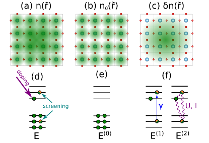
Figure 1: (Color online) Schematic cartoon that represents the key physical concepts for the development of the second-principles models: the reference atomic structure and the reference and deformation electron densities. Panels (a)-(c): the meaning of the balls (which represent the position of the atoms in a hypothetical semiconductor), and the green clouds (which represent charge densities) are explained in the main text. Panels (d)-(f): the horizontal lines represent the one-electron energy levels obtained at the corresponding atomic structures and for the reference electronic configuration (neutral ground state). Full green circles represent full occupation of a given state by electrons. Half filled orange/green circles indicate partial occupation of a particular level. The notations $E^{(0)}$, $E^{(1)}$, and $E^{(2)}$ for the energies are introduced in Sec. II.2. The parameters $\gamma$, $U$, and, $I$ are defined in Secs. II.3 and II.4. Only the case of doping with electrons is sketched. Doping with holes would lead to an equivalent picture.

In order to further clarify the concept of RED, let us discuss the application of our method to the relevant case of a doped semiconductor. As sketched in Fig. 1, our hypothetical semiconductor is made of two different types of atoms (represented by large green and small red balls, respectively) in a square planar geometry with a three-atom repeated cell. The RAG corresponds to the high-symmetry configuration in which the large atom is located at the center of the square, while the small atoms lie at the centers of the sides. In the neutral (undoped) case, a self-consistent DFT calculation of the RAG would yield an electronic configuration with all the valence bands occupied and all the conduction bands empty, as illustrated in Fig. 1(e). The associated electron density would be our RED, $n_{0}(\vec{r})$, represented by the green clouds in Fig. 1(b); the associated energy would be $E^{(0)}$, using the notation that will be introduced in Sec. II.2.

Now, if we dope the neutral system by adding or removing electrons, there will be a response of the electronic cloud, which will tend to screen the field caused by the extra charge. The doping electron (respectively, hole) will occupy the states at the bottom of the conduction band (respectively, top of the valence band). The doping-induced charge redistribution can be viewed as resulting from an admixture of occupied and unoccupied states of the reference neutral configuration. The resulting state, described by the total charge density $n(\vec{r})$, is sketched in Figs. 1(a) and 1(d). The difference between the total electronic density and the RED is the deformation density $\delta n(\vec{r})$. Such a deformation density, which is the key quantity in our scheme, captures both the doping and the system’s response to it, as sketched in Figs. 1(c) and 1(f).

Finally, let us further stress the independence between RAG and RED. Note that all three quantities $n(\vec{r})$, $n_{0}(\vec{r})$, and $\delta n(\vec{r})$ are in fact parametric functions of the atomic positions. This is illustrated in Fig. 2, which sketches a case in which one atom is displaced from the RAG.

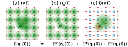
Figure 2: (Color online) Schematic cartoon emphasizing that the the division of the electron density into reference and deformation parts is carried out for any geometrical configuration of the system, as defined by the strain $\overleftrightarrow{\eta}$ and atomic displacements $\{\vec{u}_{\bm{\lambda}}\}$. The distortion of the reference atomic geometry is illustrated by the off-centering of one atom (indicated with a black arrow). The atomic distortion results in a modified $n_{0}(\vec{r})$ [panel (b)], as well as in additional changes depicted in panel (c), where the green and orange clouds denote positive and negative variations in the electronic density. Symbols have the same meaning as in Fig. 1.

II.2 Approximate expression for the energy

Let us consider an atomic geometry characterized by the homogeneous strain tensor, $\overleftrightarrow{\eta}$, and the individual atomic displacements, $\{\vec{u}_{\bm{\lambda}}\}$, as described in Eq. (1). Our main objective is to find a functional form that permits an accurate approximation of the DFT total energy at a low computational cost. The DFT energy can be written as

$$E_{\text{DFT}}= \sum_{j\vec{k}}o_{j\vec{k}}\left\langle\psi_{j\vec{k}}\right|\hat{t}+v_{\text{ext}}\left|\psi_{j\vec{k}}\right\rangle$$

$$+\frac{1}{2}\iint\frac{n(\vec{r})n(\vec{r}\mkern 2.0mu\vphantom{r}^{\prime})}{|\vec{r}-\vec{r}\mkern 2.0mu\vphantom{r}^{\prime}|}d^{3}rd^{3}r^{\prime}+E_{\text{xc}}[n]+E_{\text{nn}}.$$ (3)

In this expression, the first term on the right-hand side includes the kinetic energy of a collection of non-interacting electrons as computed through the one-particle kinetic energy operator, $\hat{t}$; this first term also includes the action of an external potential, $v_{\text{ext}}$, which gathers contributions from the nuclei (or ionic cores) and, possibly, other external fields. The second term is the Coulomb electrostatic energy, which in the context of quantum mechanics of condensed matter systems is also referred to as the Hartree term. The third term, $E_{\text{xc}}[n]$, is the so-called exchange and correlation functional, which contains the correlation contribution to the kinetic energy in the interacting electron system, as well as any electron-electron interaction effect beyond the classic Coulomb repulsion. The last term, $E_{\text{nn}}$, is the nucleus-nucleus electrostatic energy. Note that Eq. (3) is written in atomic units, which are used throughout the manuscript. ($|e|=m_{e}=\hbar=a_{\rm B}=1$, where $|e|$ is the magnitude of the electronic charge, $m_{e}$ is the electronic mass, and $a_{\rm B}$ is the Bohr radius).

As already mentioned, we assume that the Born-Oppenheimer approximation applies, so that the positions of the nuclei can be considered as parameters of the Hamiltonian. We also assume periodic boundary conditions. (Finite systems can be trivially considered by, e.g., adopting a supercell approach.Payne et al. (1992))

Within periodic boundary conditions, the eigenfunctions of the one-particle Kohn-Sham equations, $|\psi_{j\vec{k}}\rangle$, can be written as Bloch states characterized by the wave vector $\vec{k}$ and the band index $j$, with the occupation of a state given by $o_{j\vec{k}}$. Note that Eq. (3) is valid for any geometric structure of the system, and we implicitly assume that the total energy ($E_{\text{DFT}}$), the one-particle eigenstates ($|\psi_{j\vec{k}}\rangle$), and all derived magnitudes (such as the electron densities $n$, $n_{0}$, and $\delta n$) depend on the structural parameters $\overleftrightarrow{\eta}$ and $\{\vec{u}_{\bm{\lambda}}\}$.

The total energy of Eq. (3) is a functional of the density which, as described in Eq. (2), can be written as the sum of a reference part, $n_{0}(\vec{r})$, and a deformation part, $\delta n(\vec{r})$. When we implement this decomposition, the linear Coulomb energy term can be trivially dealt with. For the non-linear exchange and correlation functional, we follow Ref. (Elstner et al., 1998) and expand $E_{\text{x}c}[n]$ around the RED as

$$E_{\text{xc}}[n]= E_{\text{xc}}[n_{0}]+\int\left.\frac{\delta E_{\text{xc}}}{\delta n(\vec{r})}\right|_{n_{0}}\delta n(\vec{r})d^{3}r$$

$$+\frac{1}{2}\iint\left.\frac{\delta^{2}E_{\text{xc}}}{\delta n(\vec{r})\delta n(\vec{r}\mkern 2.0mu\vphantom{r}^{\prime})}\right|_{n_{0}}\delta n(\vec{r})\delta n(\vec{r}\mkern 2.0mu\vphantom{r}^{\prime})d^{3}rd^{3}r^{\prime}+\cdots,$$ (4)

where we have introduced functional derivatives of $E_{\text{xc}}$. In principle, Eq. (4) is exact if we consider all the orders in the expansion. (Expansions like this one are frequently found in the formulations of the adiabatic density functional perturbation theory.Gonze (1995, 1997)) In practice, under the assumption of a small deformation density, the expansion can be cut at second order. As we shall show in Secs. II.4 and II.8, this approximation includes as a particular case the full Hartree-Fock-theory; hence, we expect it to be accurate enough for our current purposes.

Within the previous approximation, we can write the total energy as a sum of terms coming from the contributions of the deformation density at zeroth (reference density), first, and second orders. Formally we write

$$E_{\text{DFT}}\approx E=E^{(0)}+E^{(1)}+E^{(2)},$$ (5)

where the individual terms have the following form. (A full derivation is given in Appendix A.)

For the zeroth-order term, $E^{(0)}$, we get

$$E^{(0)}= \sum_{j\vec{k}}o_{j\vec{k}}^{(0)}\left\langle\psi_{j\vec{k}}^{(0)}\right|\hat{t}+v_{\text{ext}}\left|\psi_{j\vec{k}}^{(0)}\right\rangle$$

$$+\frac{1}{2}\iint\frac{n_{0}(\vec{r})n_{0}(\vec{r}\mkern 2.0mu\vphantom{r}^{\prime})}{|\vec{r}-\vec{r}\mkern 2.0mu\vphantom{r}^{\prime}|}d^{3}rd^{3}r^{\prime}+E_{\text{xc}}[n_{0}]+E_{nn}.$$ (6)

The above equation corresponds, without approximation, to the exact DFT energy for the reference density, $n_{0}$. We can choose the RED so that $E^{(0)}$ is the dominant contribution to the total energy of the system, and here comes a key advantage of our approach: We can compute $E^{(0)}$ by employing a model potential that depends only on the atomic positions, where the electrons (assumed to remain on the Born-Oppenheimer surface) are integrated out. This represents a huge gain with respect to other schemes that, like the typical DFTB schemes, require an explicit and accurate treatment of the electronic interactions yielding the RED as well as solving numerically for $E^{(0)}$ and $n_{0}$ for each atomic configuration considered in the simulation.

The first-order term involves the one-electron excitations as captured by the deformation density,

$$E^{(1)}=\sum_{j\vec{k}}\left[o_{j\vec{k}}\left\langle\psi_{j\vec{k}}\right|\hat{h}_{0}\left|\psi_{j\vec{k}}\right\rangle-o_{j\vec{k}}^{(0)}\left\langle\psi_{j\vec{k}}^{(0)}\right|\hat{h}_{0}\left|\psi_{j\vec{k}}^{(0)}\right\rangle\right].$$ (7)

Here, $\hat{h}_{0}$ is the Kohn-ShamKohn and Sham (1965) one-electron Hamiltonian defined for the RED,

$$\hat{h}_{0}=\hat{t}+v_{\text{ext}}-v_{\text{H}}(n_{0};\vec{r})+v_{\text{xc}}[n_{0};\vec{r}],$$ (8)

where $v_{\text{H}}(n_{0};\vec{r})$ and $v_{\text{xc}}[n_{0};\vec{r}]$ are, respectively, the reference Hartree,

$$v_{\text{H}}(n_{0};\vec{r})=-\int\frac{n_{0}(\vec{r}\mkern 2.0mu\vphantom{r}^{\prime})}{|\vec{r}-\vec{r}\mkern 2.0mu\vphantom{r}^{\prime}|}d^{3}r^{\prime},$$ (9)

and exchange-correlation,

$$v_{\text{xc}}[n_{0};\vec{r}]=\left.\frac{\delta E_{\text{xc}}[n]}{\delta n(\vec{r})}\right|_{n_{0}},$$ (10)

potentials. It is important to note that Eq. (7) is different from the one usually employed in DFTB methods (see, for example, Refs. Porezag et al., 1995 and Elstner et al., 1998): while typical DFTB schemes include a plain sum of one-electron energies, here we deal with the difference between the value of this quantity for the actual system and for the reference one [see sketch in Fig. 1(f)]. Such a difference is a much smaller quantity, more amenable to accurate calculations.

Finally, the two-electron contribution from the deformation density, $E^{(2)}$, is given by

$$E^{(2)}=\frac{1}{2}\int d^{3}r\int d^{3}r^{\prime}g(\vec{r},\vec{r}\mkern 2.0mu\vphantom{r}^{\prime})\delta n(\vec{r})\delta n(\vec{r}\mkern 2.0mu\vphantom{r}^{\prime}),$$ (11)

where the screened electron-electron interaction operator, $g(\vec{r},\vec{r}\mkern 2.0mu\vphantom{r}^{\prime})$, is

$$g(\vec{r},\vec{r}\mkern 2.0mu\vphantom{r}^{\prime})=\frac{1}{|\vec{r}-\vec{r}\mkern 2.0mu\vphantom{r}^{\prime}|}+\left.\frac{\delta^{2}E_{\text{xc}}}{\delta n(\vec{r})\delta n(\vec{r}\mkern 2.0mu\vphantom{r}^{\prime})}\right|_{n_{0}}.$$ (12)

Here, $\delta^{2}E_{\text{xc}}/\delta n(\vec{r})\delta n(\vec{r}\mkern 2.0mu\vphantom{r}^{\prime})$ captures the effective screening of the two-electron interactions due to exchange and correlation. The latter magnitude is particularly important in chemistry, as it is related to the hardness of a material.Parr and Pearson (1983)

In summary, in this Section we have shown how a particular splitting of the total density, into reference and a deformation parts, allows us to expand the DFT energy around $n_{0}$ and as a function of $\delta n$. This expansion can be truncated at second-order while keeping a high accuracy; nevertheless, this approach can be systematically improved by including higher-order terms in $\delta n$, in analogy to what is done, e.g., in the so-called DFTB3 method.Gaus et al. (2011) While the general idea is reminiscent of DFTB methods in the literature,Porezag et al. (1995); Matthew et al. (1989); Elstner et al. (1998) our scheme has two distinct advantages. On one hand, the zeroth-order term can be conveniently parametrized by means of a lattice model potential, so that it can be evaluated in a fast and accurate way without explicit consideration of the electrons. On the other hand, the first-order term is much smaller, and can be calculated more accurately, than in usual DFTB schemes, as it takes the form of a perturbative correction.

II.3 Formulation in a Wannier basis

II.3.1 Choice of Wannier functions

Our formulation requires the computation of the matrix elements of the Kohn-Sham one-electron Hamiltonian, as defined for the RED, in terms of Bloch wavefunctions [Eq. (7)], as well as various integrals involving the deformation charge density [Eq. (11)]. To compute these terms, we will expand the Bloch waves on a basis of Wannier-like functions (WFs), $\left|\chi_{\bm{a}}\right\rangle$, in the spirit of Ref. Souza et al., 2001. There are several reasons for our choice of a Wannier basis set over the atomic orbitals most commonly used in DFTB formulations.Porezag et al. (1995); Matthew et al. (1989); Elstner et al. (1998); Lewis et al. (2011)

First, the Wannier orbitals are naturally adapted to the specific material under investigation. In fact, they will be typically obtained from a full first-principles simulation of the band structure of the target material, which permits a more accurate parametrization of the system while retaining a minimal basis set.

Second, the Wannier functions can be chosen to be spatially localized, and several localization schemes are available in the literature.Callaway and Hughes (1967); Teichler (1971); Satpathy and Pawlowska (1988); Marzari and Vanderbilt (1997); Souza et al. (2001); Sakura (2013); Wang et al. (2014) The localization will be exploited in our second-principles method to restrict the real-space matrix elements to those involving relatively close neighbors, as will be explained in Sec. III.

Third, the localized Wannier functions can be chosen to be orthogonal. Note that methods with non-orthogonal basis functions require the calculation of the overlap integrals that have a non-trivial behavior as a function of the geometry of the system. Moreover, the one-particle Kohn-Sham equations in matrix form become a generalized eigenvalue problem, whose solution requires a computationally demanding inversion of the overlap matrix. The use of orthogonal Wannier functions allows to bypass these shortcomings.

Fourth, the Wannier functions enable a very flexible description of the electronic band structure, as they can be constructed to span the space corresponding to a specific set of bands.Souza et al. (2001); Marzari et al. (2012) Therefore, the electronic states can be efficiently split into: (i) an active set playing an important role in the properties under study; and (ii) a background set that will be integrated out from the explicit treatment. For instance, if the problem of interest involves the formation of low-energy electron-hole excitons, our active set would be comprised by the top-valence and bottom-conduction bands, and we would use the corresponding Wannier functions as a basis set.

Typically, we will start from a set of Bloch-like Hamiltonian eigenstates, $|\psi_{n\vec{k}}^{(0)}\rangle$, that define a manifold of $J$ bands associated to the RED. Then, following e.g. the recipe of Ref. Marzari and Vanderbilt, 1997, we have

$$|\chi_{\bm{a}}\rangle\equiv|\vec{R}_{A}a\rangle=\frac{V}{\left(2\pi\right)^{3}}\int_{\rm BZ}d\vec{k}\>\>e^{-i\vec{k}\cdot\vec{R}_{A}}\sum_{m=1}^{J}T_{ma}^{(\vec{k})}|\psi_{m\vec{k}}^{(0)}\rangle,$$ (13)

where the Wannier function $|\vec{R}_{A}a\rangle$ is labeled by the cell $A$ at which it is centered (associated to the lattice vector $\vec{R}_{A}$) and by a discrete index $a$. Note that we use Latin subindices to label all physical quantities related with the electrons; to alleviate the notation, we group in the bold symbol $\bm{a}$ both the cell and the discrete index, so that $\bm{a}\leftrightarrow\vec{R}_{A}a$. In Eq. (13), $V$ is the volume of the primitive unit cell, the integral is carried out over the whole Brillouin zone ($\rm BZ$), the index $m$ runs over all the $J$ bands of the manifold, and the $\bm{T}^{(\vec{k})}$ matrices represent unitary transformations among the $J$ Bloch orbitals at a given wavevector.

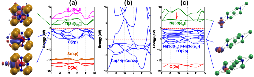
Figure 3: (Color online) Band structure, showing different band entanglements, in three archetypal cases: (a) insulating SrTiO₃, (b) metallic Cu, and (c) antiferromagnetic NiO. The groups of entangled bands are separated by energy gaps and colored differently. For SrTiO₃: bands with dominant O($2s$), Sr($4p$), O($2p$), Ti[$3d(t_{2g})$], and Ti[$3d(e_{g})$] characters are plotted, respectively in red, orange, blue, green, and magenta. For Cu: all the bands are entangled. For NiO: some weakly-disperssive bands at the top of the valence and bottom of the conduction regions (indicated by an arrow) share the Ni[$3d(e_{g})$] character. On the leftmost and rightmost edges of the figure, the spatial shape of some of the Wannier functions for SrTiO₃ and NiO are displayed, respectively. Isosurfaces corresponding to positive and negative values of the MLWFs are plotted with different colors. In these diagrams, golden, blue, red, and green spheres represent, respectively, Sr, O, Ti, and Ni ions. For NiO, the atoms in the cell used to simulate the antiferromagnetic ground state are shown. Dashed red lines mark the Fermi energy of the metal and the top of the valence bands of the insulators; in all cases such level is taken as the zero of energy.

Figure 3 shows three paradigmatic examples: a non-magnetic insulator [bulk SrTiO₃, Fig. 3(a)], a non-magnetic metal [bulk Cu, Fig. 3(b)], and an antiferromagnetic insulator [bulk NiO, Fig. 3(c)].

In the first case, the valence bands are well separated in energy from other bands; further, they have a well-defined character strongly reminiscent of the corresponding atomic orbitals. More precisely, three isolated manifolds corresponding to the occupied valence bands – with dominant O-$2s$, Sr-$4p$, and O-$2p$ character, respectively – are clearly visible; these bands are centered around 17 eV, 15 eV, and 3 eV below the valence-band top, respectively. The Bloch eigenstates for these bands can be directly used to compute the corresponding localized Wannier functions following the scheme of Ref. Marzari and Vanderbilt, 1997 or similar ones. In contrast, the bottom conduction bands of SrTiO₃ have a dominant Ti-$t_{2g}$ character, but overlap in energy with higher-lying (Ti-$e_{g}$) conduction bands. The situation is even more complicated in the cases of Figs. 3(b) and 3(c), where the critical bands – i.e., those around the Fermi energy in the case of Cu, and those comprising the Ni-$3d$ manifold in the case of NiO – are strongly entangled with other states. In such cases, we may need to use a disentanglement method – like e.g. the one proposed in Ref. Souza et al., 2001 – to identify a minimal active manifold.

Note that the inverse transformation from Wannier to Bloch functions reads

$$|\psi_{j\vec{k}}^{(0)}\rangle=\sum_{{\bm{a}}}c_{ja\vec{k}}^{(0)}e^{i\vec{k}\cdot\vec{R}_{A}}|\chi_{\bm{a}}\rangle,$$ (14)

where the connection between the $c_{ja\vec{k}}^{(0)}$ coefficients and the transformation matrices in Eq. (13) is given in Appendix B.

The Wannier functions corresponding to the RED [Fig. 1(b)] form a complete basis of the Hilbert space. Hence, we can use them to represent any perturbed electronic configuration of the system [e.g., the one sketched in Fig. 1(a)] as

$$|\psi_{j\vec{k}}\rangle=\sum_{{\bm{a}}}c_{ja\vec{k}}e^{i\vec{k}\cdot\vec{R}_{A}}|\chi_{\bm{a}}\rangle,$$ (15)

where the sum can be extended to as many bands as needed to accurately describe the phenomenon of interest. (As in the example of Fig. 1, this might be the addition of an electron and the associated screening.)

Finally, note that the Wannier function basis is implicitly dependent on the structural parameters $\overleftrightarrow{\eta}$ and $\{\vec{u}_{\bm{\lambda}}\}$, and it should be recomputed for every new RED corresponding to varying atomic positions. Ultimately, our models will capture all such effects implicitly in the electron-lattice coupling terms, whose calculation is described in Sec. II.6.

Also, henceforth we will assume that each and every one of the WFs in our basis can be unambiguously associated with a particular atom at (around) which it is centered. Further, we will use the notation $\bm{a}\in\bm{\lambda}$ to refer to all the WFs associated to atom $\lambda$ in cell $\Lambda$, an identification that will be necessary when discussing our treatment of electrostatic couplings in Sec. II.5.

II.3.2 Equations in a Wannier basis

Using Eq. (15), we can write the electron density $n(\vec{r})$ in terms of the Wannier functions,

$$n(\vec{r}) =\sum_{j\vec{k}}o_{j\vec{k}}|\psi_{j\vec{k}}(\vec{r})|^{2}=\sum_{j\vec{k}}o_{j\vec{k}}\psi^{*}_{j\vec{k}}(\vec{r})\psi_{j\vec{k}}(\vec{r})$$

$$=\sum_{j\vec{k}}\sum_{\bm{a}\bm{b}}o_{j\vec{k}}c_{ja\vec{k}}^{*}c_{jb\vec{k}}e^{i\vec{k}(\vec{R}_{B}-\vec{R}_{A})}\chi_{\bm{a}}(\vec{r})\chi_{\bm{b}}(\vec{r})$$

$$=\sum_{\bm{a}\bm{b}}d_{\bm{a}\bm{b}}\chi_{\bm{a}}(\vec{r})\chi_{\bm{b}}(\vec{r}).$$ (16)

We can assume we will work with real Wannier functionsMarzari et al. (2012) and therefore drop the complex conjugates in our equations. In Eq. (16) we have introduced a reduced density matrix,

$$d_{\bm{a}\bm{b}}=\sum_{j\vec{k}}o_{j\vec{k}}c_{ja\vec{k}}^{*}c_{jb\vec{k}}e^{i\vec{k}(\vec{R}_{B}-\vec{R}_{A})},$$ (17)

which, following the nomenclature of Ref. Marzari et al., 1997, will be referred to as the occupation matrix for the WFs. This occupation matrix has the usual properties, including periodicity when the Wannier functions are displaced by the same lattice vector in real space.

Equation (16) can similarly be applied to the RED,

$$n_{0}(\vec{r})=\sum_{\bm{a}\bm{b}}d_{\bm{a}\bm{b}}^{(0)}\chi_{\bm{a}}(\vec{r})\chi_{\bm{b}}(\vec{r}),$$ (18)

where the calculation of the occupation matrix is performed with the coefficients of the Bloch functions that define the reference electronic density, $c_{j\alpha\vec{k}}^{(0)}$, as in Eq. (14).

In order to quantify the difference between the two densities defined in Eqs. (16) and (18), we introduce a deformation occupation matrix,

$$D_{\bm{a}\bm{b}}=d_{\bm{a}\bm{b}}-d_{\bm{a}\bm{b}}^{(0)},$$ (19)

which will be the central magnitude in our calculations. Now the deformation density can be written as

$$\delta n(\vec{r})=\sum_{\bm{a}\bm{b}}D_{\bm{a}\bm{b}}\chi_{\bm{a}}(\vec{r})\chi_{\bm{b}}(\vec{r}).$$ (20)

Using these definitions, we can rewrite the $E^{(1)}$ and $E^{(2)}$ energy terms. Introducing Eq. (19) into Eqs. (7) and (11) we get

$$E^{(1)}= \sum_{j\vec{k}}\left[o_{j\vec{k}}\left\langle\psi_{j\vec{k}}\right|\hat{h}_{0}\left|\psi_{j\vec{k}}\right\rangle-o_{j\vec{k}}^{(0)}\left\langle\psi_{j\vec{k}}^{(0)}\right|\hat{h}_{0}\left|\psi_{j\vec{k}}^{(0)}\right\rangle\right]$$

$$= \sum_{j\vec{k}}\left[o_{j\vec{k}}\sum_{\bm{a}\bm{b}}c^{*}_{aj\vec{k}}c_{bj\vec{k}}e^{i\vec{k}(\vec{R}_{B}-\vec{R}_{A})}\langle\chi_{\bm{a}}|\hat{h}_{0}|\chi_{\bm{b}}\rangle\right.$$

$$-\left.o^{(0)}_{j\vec{k}}\sum_{\bm{a}\bm{b}}\left(c^{(0)}_{aj\vec{k}}\right)^{*}c^{(0)}_{bj\vec{k}}e^{i\vec{k}(\vec{R}_{B}-\vec{R}_{A})}\langle\chi_{\bm{a}}|\hat{h}_{0}|\chi_{\bm{b}}\rangle\right]$$

$$= \left[\sum_{\bm{a}\bm{b}}d_{\bm{a}\bm{b}}\langle\chi_{\bm{a}}|\hat{h}_{0}|\chi_{\bm{b}}\rangle-\sum_{\bm{a}\bm{b}}d^{(0)}_{\bm{a}\bm{b}}\langle\chi_{\bm{a}}|\hat{h}_{0}|\chi_{\bm{b}}\rangle\right]$$

$$= \sum_{\bm{a}\bm{b}}D_{\bm{a}\bm{b}}\gamma_{\bm{a}\bm{b}},$$ (21)

and

$$E^{(2)} =\frac{1}{2}\int d^{3}r\int d^{3}r^{\prime}g(\vec{r},\vec{r}\mkern 2.0mu\vphantom{r}^{\prime})\delta n(\vec{r})\delta n(\vec{r}\mkern 2.0mu\vphantom{r}^{\prime})$$

$$=\frac{1}{2}\sum_{\bm{a}\bm{b}}\sum_{\bm{a}^{\prime}\bm{b}^{\prime}}D_{\bm{a}\bm{b}}D_{\bm{a}^{\prime}\bm{b}^{\prime}}\langle\chi_{\bm{a}}\chi_{\bm{a}^{\prime}}|\hat{g}|\chi_{\bm{b}}\chi_{\bm{b}^{\prime}}\rangle$$

$$=\frac{1}{2}\sum_{\bm{a}\bm{b}}\sum_{\bm{a}^{\prime}\bm{b}^{\prime}}D_{\bm{a}\bm{b}}D_{\bm{a}^{\prime}\bm{b}^{\prime}}U_{\bm{a}\bm{b}\bm{a}^{\prime}\bm{b}^{\prime}},$$ (22)

respectively, where $\gamma_{\bm{a}\bm{b}}$ and $U_{\bm{a}\bm{b}\bm{a}^{\prime}\bm{b}^{\prime}}$ are the primary parameters that define our electronic model. These parameters can be obtained, respectively, from the integrals of the one- and two-electron operators computed in DFT simulations, as

$$\gamma_{\bm{a}\bm{b}} =\left\langle\chi_{\bm{a}}\right|\hat{h}_{0}\left|\chi_{\bm{b}}\right\rangle$$

$$=\int d^{3}r\>\chi_{\bm{a}}(\vec{r})\>h_{0}(\vec{r})\>\chi_{\bm{b}}(\vec{r}),$$ (23)

and

$$U_{\bm{a}\bm{b}\bm{a}^{\prime}\bm{b}^{\prime}} =\langle\chi_{\bm{a}}\chi_{\bm{a}^{\prime}}|\hat{g}|\chi_{\bm{b}}\chi_{\bm{b}^{\prime}}\rangle$$

$$=\int d^{3}r\int d^{3}r^{\prime}\chi_{\bm{a}}(\vec{r})\chi_{\bm{b}}(\vec{r})\chi_{\bm{a}^{\prime}}(\vec{r}\mkern 2.0mu\vphantom{r}^{\prime})\chi_{\bm{b}^{\prime}}(\vec{r}\mkern 2.0mu\vphantom{r}^{\prime})g(\vec{r},\vec{r}\mkern 2.0mu\vphantom{r}^{\prime}).$$ (24)

Alternatively, they can be fitted so that the model reproduces a training set of first-principles data.

II.4 Magnetic systems

The above expressions are valid for systems without spin polarization. The procedure to construct the energy for magnetic cases is very similar, but there are subtleties pertaining the choice of RED.

In principle, one could use a RED corresponding to a particular realization of the spin order, e.g., the anti-ferromagnetic ground state for a typical magnetic insulator, or the ferromagnetic ground state for a typical magnetic metal. However, such a choice is likely to result in a less accurate description of other spin arrangements, which would hamper the application of the model to investigate certain phenomena (e.g., a spin-ordering transition).

Alternatively, one might adopt a non-magnetic RED around which to construct the model. Such a RED might correspond to an actual computable state: for example, it could be obtained from a non-magnetic DFT simulation in which a perfect pairing of spin-up and spin-down electrons is imposed. Further, as we will see below for the case of NiO, in some cases it is possible and convenient to consider a virtual RED whose character can be inspected a posteriori. This latter option follows the spirit of the usual approach to the construction of spin-phonon effective Hamiltonians, Cazorla and Íñiguez (2013) where the parameters defining the reference state cannot be computed directly from DFT, but are effectively fitted by requesting the model to reproduce the properties of specific spin arrangements.

In the following we assume a non-magnetic RED, and present an otherwise general formulation.

The $E^{(0)}$ and $E^{(1)}$ terms thus describe the lattice and one-electron energetics corresponding to the non-magnetic RED, and do not capture any effect related with the spin polarization. In contrast, the screened electron-electron interaction operator [Eq. (12)] is spin dependent and equal to

$$g(\vec{r},\vec{r}\mkern 2.0mu\vphantom{r}^{\prime},s,s^{\prime})=\frac{1}{|\vec{r}-\vec{r}\mkern 2.0mu\vphantom{r}^{\prime}|}+\left.\frac{\delta^{2}E_{\text{xc}}}{\delta n(\vec{r},s)\delta n(\vec{r}\mkern 2.0mu\vphantom{r}^{\prime},s^{\prime})}\right|_{n_{0}}.$$ (25)

where $s$ and $s^{\prime}$ are spin indices that can take “up” or “down” values which we denote, respectively, by $\uparrow$ and $\downarrow$ symbols. This distinction in the screened electron-electron operator leads us to introduce two kinds of $U$ parameters,

$$U_{\bm{a}\bm{b}\bm{a}^{\prime}\bm{b}^{\prime}}^{\text{par}} =\int d^{3}r\int d^{3}r^{\prime}\chi_{\bm{a}}(\vec{r})\chi_{\bm{b}}(\vec{r})\chi_{\bm{a}^{\prime}}(\vec{r}\mkern 2.0mu\vphantom{r}^{\prime})\chi_{\bm{b}^{\prime}}(\vec{r}\mkern 2.0mu\vphantom{r}^{\prime})g(\vec{r},\vec{r}\mkern 2.0mu\vphantom{r}^{\prime},\uparrow,\uparrow)$$

$$=\int d^{3}r\int d^{3}r^{\prime}\chi_{\bm{a}}(\vec{r})\chi_{\bm{b}}(\vec{r})\chi_{\bm{a}^{\prime}}(\vec{r}\mkern 2.0mu\vphantom{r}^{\prime})\chi_{\bm{b}^{\prime}}(\vec{r}\mkern 2.0mu\vphantom{r}^{\prime})g(\vec{r},\vec{r}\mkern 2.0mu\vphantom{r}^{\prime},\downarrow,\downarrow)$$

and

$$U_{\bm{a}\bm{b}\bm{a}^{\prime}\bm{b}^{\prime}}^{\text{anti}} =\int d^{3}r\int d^{3}r^{\prime}\chi_{\bm{a}}(\vec{r})\chi_{\bm{b}}(\vec{r})\chi_{\bm{a}^{\prime}}(\vec{r}\mkern 2.0mu\vphantom{r}^{\prime})\chi_{\bm{b}^{\prime}}(\vec{r}\mkern 2.0mu\vphantom{r}^{\prime})g(\vec{r},\vec{r}\mkern 2.0mu\vphantom{r}^{\prime},\uparrow,\downarrow)$$

$$=\int d^{3}r\int d^{3}r^{\prime}\chi_{\bm{a}}(\vec{r})\chi_{\bm{b}}(\vec{r})\chi_{\bm{a}^{\prime}}(\vec{r}\mkern 2.0mu\vphantom{r}^{\prime})\chi_{\bm{b}^{\prime}}(\vec{r}\mkern 2.0mu\vphantom{r}^{\prime})g(\vec{r},\vec{r}\mkern 2.0mu\vphantom{r}^{\prime},\downarrow,\uparrow),$$

which describe, respectively, the interactions between electrons with parallel ($U^{\text{par}}$) and antiparallel ($U^{\text{anti}}$) spins. As a consequence, $E^{(2)}$ in spin-polarized systems is

$$E^{(2)} =\sum_{s,s^{\prime}}\frac{1}{2}\int d^{3}r\int d^{3}r^{\prime}g({r},\vec{r}\mkern 2.0mu\vphantom{r}^{\prime},s,s^{\prime})\delta n(\vec{r},s)\delta n(\vec{r}\mkern 2.0mu\vphantom{r}^{\prime},s^{\prime}),$$ (28)

where

$$\delta n(\vec{r},s)=\sum_{\bm{a}\bm{b}}D_{\bm{a}\bm{b}}^{s}\chi_{\bm{a}}(\vec{r})\chi_{\bm{b}}(\vec{r}),$$ (29)

and $D_{\bm{a}\bm{b}}^{s}$ is the deformation occupation matrix for the $s$ spin-channel, defined for the up and down spins as

$$D_{\bm{a}\bm{b}}^{\uparrow} =d_{\bm{a}\bm{b}}^{\uparrow}-\frac{1}{2}d_{\bm{a}\bm{b}}^{(0)}$$ (30)

and

$$D_{\bm{a}\bm{b}}^{\downarrow} =d_{\bm{a}\bm{b}}^{\downarrow}-\frac{1}{2}d_{\bm{a}\bm{b}}^{(0)},$$ (31)

respectively. Replacing Eqs. (29)-(31) into Eq. (28),

$$E^{(2)}= \frac{1}{2}\sum_{s,s^{\prime}}\sum_{\bm{a}\bm{b}}\sum_{\bm{a}^{\prime}\bm{b}^{\prime}}D_{\bm{a}\bm{b}}^{s}D_{\bm{a}^{\prime}\bm{b}^{\prime}}^{s^{\prime}}$$

$$\int d^{3}r\int d^{3}r^{\prime}\chi_{\bm{a}}(\vec{r})\chi_{\bm{b}}(\vec{r})\chi_{\bm{a}^{\prime}}(\vec{r}\mkern 2.0mu\vphantom{r}^{\prime})\chi_{\bm{b}^{\prime}}(\vec{r}\mkern 2.0mu\vphantom{r}^{\prime})g({r},\vec{r}\mkern 2.0mu\vphantom{r}^{\prime},s,s^{\prime})$$

$$= \frac{1}{2}\left\{\sum_{\bm{a}\bm{b}}\sum_{\bm{a}^{\prime}\bm{b}^{\prime}}\left[D_{\bm{a}\bm{b}}^{\uparrow}D_{\bm{a}^{\prime}\bm{b}^{\prime}}^{\uparrow}+D_{\bm{a}\bm{b}}^{\downarrow}D_{\bm{a}^{\prime}\bm{b}^{\prime}}^{\downarrow}\right]\right.U_{\bm{a}\bm{b}\bm{a}^{\prime}\bm{b}^{\prime}}^{\text{par}}+$$

$$\left.\left[D_{\bm{a}\bm{b}}^{\uparrow}D_{\bm{a}^{\prime}\bm{b}^{\prime}}^{\downarrow}+D_{\bm{a}\bm{b}}^{\downarrow}D_{\bm{a}^{\prime}\bm{b}^{\prime}}^{\uparrow}\right]U_{\bm{a}\bm{b}\bm{a}^{\prime}\bm{b}^{\prime}}^{\text{anti}}\right\}$$ (32)

For physical clarity, and to establish the link of Eqs. (LABEL:eq:Upar) and (LABEL:eq:Uanti) with Eq. (24), it is convenient to write $U^{\text{par}}$ and $U^{\text{anti}}$ in terms of Hubbard- ($U$) and Stoner- ($I$) like parameters:

$$U^{\text{par}}_{\bm{a}\bm{b}\bm{a}^{\prime}\bm{b}^{\prime}} = U_{\bm{a}\bm{b}\bm{a}^{\prime}\bm{b}^{\prime}}-I_{\bm{a}\bm{b}\bm{a}^{\prime}\bm{b}^{\prime}}$$ (33)

$$U^{\text{anti}}_{\bm{a}\bm{b}\bm{a}^{\prime}\bm{b}^{\prime}} = U_{\bm{a}\bm{b}\bm{a}^{\prime}\bm{b}^{\prime}}+I_{\bm{a}\bm{b}\bm{a}^{\prime}\bm{b}^{\prime}},$$ (34)

so

$$U_{\bm{a}\bm{b}\bm{a}^{\prime}\bm{b}^{\prime}} = \frac{1}{2}\left(U^{\text{par}}_{\bm{a}\bm{b}\bm{a}^{\prime}\bm{b}^{\prime}}+U^{\text{anti}}_{\bm{a}\bm{b}\bm{a}^{\prime}\bm{b}^{\prime}}\right),$$ (35)

$$I_{\bm{a}\bm{b}\bm{a}^{\prime}\bm{b}^{\prime}} = \frac{1}{2}\left(U^{\text{anti}}_{\bm{a}\bm{b}\bm{a}^{\prime}\bm{b}^{\prime}}-U^{\text{par}}_{\bm{a}\bm{b}\bm{a}^{\prime}\bm{b}^{\prime}}\right).$$ (36)

It is also convenient to introduce

$$D_{\bm{a}^{\prime}\bm{b}^{\prime}}^{U}=D_{\bm{a}^{\prime}\bm{b}^{\prime}}^{\uparrow}+D_{\bm{a}^{\prime}\bm{b}^{\prime}}^{\downarrow},$$ (37)

and

$$D_{\bm{a}^{\prime}\bm{b}^{\prime}}^{I}=D_{\bm{a}^{\prime}\bm{b}^{\prime}}^{\uparrow}-D_{\bm{a}^{\prime}\bm{b}^{\prime}}^{\downarrow},$$ (38)

so that Eq. (32) can be rewritten as:

$$E^{(2)}=\frac{1}{2}\sum_{\bm{a}\bm{b}}\sum_{\bm{a}^{\prime}\bm{b}^{\prime}} \left\{D_{\bm{a}\bm{b}}^{U}D_{\bm{a}^{\prime}\bm{b}^{\prime}}^{U}U_{\bm{a}\bm{b}\bm{a}^{\prime}\bm{b}^{\prime}}-D_{\bm{a}\bm{b}}^{I}D_{\bm{a}^{\prime}\bm{b}^{\prime}}^{I}I_{\bm{a}\bm{b}\bm{a}^{\prime}\bm{b}^{\prime}}\right\}.$$ (39)

Note that the value of $U$ in Eqs. (33) and (34) is consistent with the one in Eq. (24) if we consider a non-spin-polarized density ($D_{\bm{a}\bm{b}}^{\downarrow}=D_{\bm{a}\bm{b}}^{\uparrow}$). In addition, note that the newly introduced constant $I_{\bm{a}\bm{b}\bm{a}^{\prime}\bm{b}^{\prime}}$ only plays a role in spin-polarized systems and is necessarily responsible for magnetism.

Connection with other schemes

The two-electron interaction constants – $U$ and $I$ defined in Eqs. (33) and (34), respectively – are formally similar to the four-index integrals typically found in Hartree-Fock theoryJensen (1999) and can be chosen to completely match this approach.

However, one should note that the electron-electron interaction in our Hubbard-like and Stoner-like constants is not the bare one, but is screened by the exchange-correlation potential associated to the reference density, $n_{0}$ [see Eq. (25)]. This fact brings our formulation closer to the so-called DFT+U Anisimov et al. (1997); Liechtenstein et al. (1995) and GWHedin (1965); Aryasetiawan and Gunnarsson (1998) methods.

Looking in more detail at our expressions for $U$ and $I$,

$$U_{\bm{a}\bm{b}\bm{a}^{\prime}\bm{b}^{\prime}} =\int d^{3}r\int d^{3}r^{\prime}\chi_{\bm{a}}(\vec{r})\chi_{\bm{b}}(\vec{r})\chi_{\bm{a}^{\prime}}(\vec{r}\mkern 2.0mu\vphantom{r}^{\prime})\chi_{\bm{b}^{\prime}}(\vec{r}\mkern 2.0mu\vphantom{r}^{\prime})g_{U}(\vec{r},\vec{r}\mkern 2.0mu\vphantom{r}^{\prime})$$ (40)

$$I_{\bm{a}\bm{b}\bm{a}^{\prime}\bm{b}^{\prime}} =\int d^{3}r\int d^{3}r^{\prime}\chi_{\bm{a}}(\vec{r})\chi_{\bm{b}}(\vec{r})\chi_{\bm{a}^{\prime}}(\vec{r}\mkern 2.0mu\vphantom{r}^{\prime})\chi_{\bm{b}^{\prime}}(\vec{r}\mkern 2.0mu\vphantom{r}^{\prime})g_{I}(\vec{r},\vec{r}\mkern 2.0mu\vphantom{r}^{\prime}),$$ (41)

we find that they are very similar to those of $U^{\text{par}}$ [Eq. (LABEL:eq:Upar)] and $U^{\text{anti}}$ [Eq. (LABEL:eq:Uanti)], except that the operator involved in the double integral is, respectively,

$$g_{U}(\vec{r},\vec{r}\mkern 2.0mu\vphantom{r}^{\prime}) =\frac{1}{|\vec{r}-\vec{r}\mkern 2.0mu\vphantom{r}^{\prime}|}+$$

$$\frac{1}{2}\left[\left.\frac{\delta^{2}E_{\text{xc}}}{\delta n(\vec{r},\uparrow)\delta n(\vec{r}\mkern 2.0mu\vphantom{r}^{\prime},\uparrow)}\right|_{n_{0}}+\left.\frac{\delta^{2}E_{\text{xc}}}{\delta n(\vec{r},\uparrow)\delta n(\vec{r}\mkern 2.0mu\vphantom{r}^{\prime},\downarrow)}\right|_{n_{0}}\right],$$ (42)

and

$$g_{I}(\vec{r},\vec{r}\mkern 2.0mu\vphantom{r}^{\prime}) =$$

$$\frac{1}{2}\left[\left.\frac{\delta^{2}E_{\text{xc}}}{\delta n(\vec{r},\uparrow)\delta n(\vec{r}\mkern 2.0mu\vphantom{r}^{\prime},\downarrow)}\right|_{n_{0}}-\left.\frac{\delta^{2}E_{\text{xc}}}{\delta n(\vec{r},\uparrow)\delta n(\vec{r}\mkern 2.0mu\vphantom{r}^{\prime},\uparrow)}\right|_{n_{0}}\right].$$ (43)

Thus, we see that $U$ contains the classical Hartree interactions, screened by exchange and correlation. Moreover, from Eq. (39) we see that $U$, as used here, is related with the deformation occupation matrix $D^{U}$, that captures the total change of the electron density (i.e., the sum of the deformation occupation matrix for both components of spins). Therefore, it is consistent with the usual definition $U=d^{2}E/dn^{2}$, i.e., it quantifies the energy needed to add or remove electrons.

On the other hand, Stoner’sStoner (1936); Gunnarson (1976); Stöhr and Siegmann (2006) $I$ only includes terms with quantum origin. In particular $g_{I}$ provides the difference in interaction between electrons with parallel and antiparallel spins.

II.5 Electrostatics

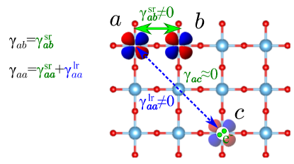
Figure 4: (Color online) Schematic representation of the near- and far-field interactions. The shape of the orbitals (represented here by two $t_{2g}$-like WFs labeled $\bm{a}$ and $\bm{b}$) is important in the determination of the short-range part of the $\gamma$ and $U$ interactions. In addition, the diagonal terms like $\gamma_{\bm{a}\bm{a}}$ and $U_{\bm{a}\bm{a}\bm{b}\bm{b}}$ also include far-field effects due to charges and dipoles at distant regions of the material (see WF $\bm{c}$ in the figure). As regards the far-field interactions, the precise shape of the charge distributions generating the potential is not critical (illustrated by the diffuse orbital at point $\bm{c}$), and can be approximated by a multipole expansion.

II.5.1 One-electron parameters

The matrix element $\gamma_{\bm{a}\bm{b}}$ [Eq. (23)] gathers Coulomb interactions associated to the electrostatic potential created by both electrons and nuclei, which acts on the WFs $\chi_{\bm{a}}$ and $\chi_{\bm{b}}$. Note that these are the only long-ranged interactions in the system, since all other contributions (kinetic, exchange-correlation, external applied fields) can be considered local or semi-local. In the following we discuss the detailed form of this electrostatic part of $\gamma_{\bm{a}\bm{b}}$, which we denote $\gamma_{\bm{a}\bm{b}}^{\rm elec}$.

Let us first consider the part of $\gamma_{\bm{a}\bm{b}}^{\rm elec}$ associated to the electrostatic potential created by the electrons, $\gamma_{\bm{a}\bm{b}}^{\text{elec,e}}$. We have

$$\gamma_{\bm{a}\bm{b}}^{\text{elec,e}} \equiv-\left\langle\chi_{\bm{a}}\right|v_{\rm H}(n_{0};\vec{r})\left|\chi_{\bm{b}}\right\rangle$$

$$=\int\chi_{\bm{a}}(\vec{r})\left(\int\frac{n_{0}(\vec{r}\mkern 2.0mu\vphantom{r}^{\prime})}{|\vec{r}-\vec{r}\mkern 2.0mu\vphantom{r}^{\prime}|}d^{3}r^{\prime}\right)\chi_{\bm{b}}(\vec{r})d^{3}r$$

$$=\int\chi_{\bm{a}}(\vec{r})\left(\int\frac{\sum_{\bm{c}}o_{\bm{c}}^{(0)}|\chi_{\bf c}(\vec{r}\mkern 2.0mu\vphantom{r}^{\prime})|^{2}}{|\vec{r}-\vec{r}\mkern 2.0mu\vphantom{r}^{\prime}|}d^{3}r^{\prime}\right)\chi_{\bm{b}}(\vec{r})d^{3}r.$$ (44)

The expression of the reference electron density in terms of the occupation of Wanniers, $o_{\bm{c}}^{(0)}$, and squares of Wannier functions in the reference state will be described in more detail in Sec. II.10. Following the criteria of Ref. Demkov et al., 1995, the one-electron matrix elements related with the Coulomb electron-electron interaction can be split into two categories: (i) the near-field regime, where the two WFs ($\bm{a}$ and $\bm{b}$) significantly overlap with the third WF ($\bm{c}$) that creates the electrostatic potential, and (ii) the far-field regime, where this overlap is negligible.

In the far-field regime, the electrostatic potential outside the region where a source charge $\chi_{\bm{c}}$ is located can be expressed as a multipole expansion (see Chapter 4 of Ref. Jackson, 1975). More precisely, we can write the far-field (FF) potential created by the charge distribution given by $\chi_{\bm{c}}$ as

$$v_{{\rm FF},{\bm{c}}}^{\rm e}(n_{0};\vec{r})=-o_{\bm{c}}^{(0)}\int\frac{|\chi_{\bm{c}}(\vec{r}\mkern 2.0mu\vphantom{r}^{\prime})|^{2}}{|\vec{r}-\vec{r}\mkern 2.0mu\vphantom{r}^{\prime}|}d^{3}r^{\prime},$$ (45)

which applies to $\vec{r}$ points for which $\chi_{\bm{c}}(\vec{r})\approx 0$. Now, let $\bm{\lambda}$ label the atom – located at the RAG reference position $\vec{\tau}_{\bm{\lambda}}=\vec{R}_{\Lambda}+\vec{\tau}_{\lambda}$ – around which $\chi_{\bm{c}}$ is centered. It is convenient to shift the origin in the integral, $\vec{r}\mkern 2.0mu\vphantom{r}^{\prime\prime}=\vec{r}\mkern 2.0mu\vphantom{r}^{\prime}-\vec{\tau}_{\bm{\lambda}}$, to write

$$v_{{\rm FF},{\bm{c}}}^{\rm e}(n_{0};\vec{r})=-o_{\bm{c}}^{(0)}\int\frac{|\chi_{\bm{c}}(\vec{r}\mkern 2.0mu\vphantom{r}^{\prime\prime}+\vec{\tau}_{\bm{\lambda}})|^{2}}{|\vec{r}-\vec{\tau}_{\bm{\lambda}}-\vec{r}\mkern 2.0mu\vphantom{r}^{\prime\prime}|}d^{3}r^{\prime\prime}.$$ (46)

Then, assuming that $|\vec{r}\mkern 2.0mu\vphantom{r}^{\prime\prime}|\ll|\vec{r}-\vec{\tau}_{\bm{\lambda}}|$ and using the superscript $T$ to indicate the transpose operation, as necessary to compute inner dot products, we get

$$\frac{1}{|\vec{r}-\vec{\tau}_{\bm{\lambda}}-\vec{r}\mkern 2.0mu\vphantom{r}^{\prime\prime}|}\approx\frac{1}{|\vec{r}-\vec{\tau}_{\bm{\lambda}}|}+\frac{(\vec{r}-\vec{\tau}_{\bm{\lambda}})^{T}\vec{r}\mkern 2.0mu\vphantom{r}^{\prime\prime}}{|\vec{r}-\vec{\tau}_{\bm{\lambda}}|^{3}}+\ldots$$ (47)

Now, substituting Eq. (47) into Eq. (46) we obtain the multipole series

$$v_{{\rm FF},{\bm{c}}}^{\rm e}(n_{0};\vec{r}) \approx-o_{\bm{c}}^{(0)}\left[\frac{\int|\chi_{\bm{c}}(\vec{r}\mkern 2.0mu\vphantom{r}^{\prime\prime}+\vec{\tau}_{\bm{\lambda}})|^{2}d^{3}r^{\prime\prime}}{|\vec{r}-\vec{\tau}_{\bm{\lambda}}|}+\right.$$

$$\left.\frac{(\vec{r}-\vec{\tau}_{\bm{\lambda}})^{T}\int|\chi_{\bm{c}}(\vec{r}\mkern 2.0mu\vphantom{r}^{\prime\prime}+\vec{\tau}_{\bm{\lambda}})|^{2}\vec{r}\mkern 2.0mu\vphantom{r}^{\prime\prime}d^{3}r^{\prime\prime}}{|\vec{r}-\vec{\tau}_{\bm{\lambda}}|^{3}}+\ldots\right]$$

$$=\frac{q_{\bm{c}}}{|\vec{r}-\vec{\tau}_{\bm{\lambda}}|}+\frac{(\vec{r}-\vec{\tau}_{\bm{\lambda}})^{T}\vec{p}_{\bm{c}}}{|\vec{r}-\vec{\tau}_{\bm{\lambda}}|^{3}}+\ldots.$$ (48)

The coefficient of the first term is the total charge (i.e., the monopole), and it is given by

$$q_{\bm{c}}=-o_{\bm{c}}^{(0)}\int|\chi_{\bm{c}}(\vec{r}\mkern 2.0mu\vphantom{r}^{\prime\prime}+\vec{\tau}_{\bm{\lambda}})|^{2}d^{3}r^{\prime\prime}=-o_{\bm{c}}^{(0)}.$$ (49)

The coefficient of the second term is the electric dipole moment associated to $\chi_{\bm{c}}$, which amounts to

$$\vec{p}_{\bm{c}} =-o_{\bm{c}}^{(0)}\int|\chi_{\bm{c}}(\vec{r}\mkern 2.0mu\vphantom{r}^{\prime\prime}+\vec{\tau}_{\bm{\lambda}})|^{2}\vec{r}\mkern 2.0mu\vphantom{r}^{\prime\prime}d^{3}r^{\prime\prime}$$

$$=-o_{\bm{c}}^{(0)}\int|\chi_{\bm{c}}(\vec{r}\mkern 2.0mu\vphantom{r}^{\prime})|^{2}(\vec{r}\mkern 2.0mu\vphantom{r}^{\prime}-\vec{\tau}_{\bm{\lambda}})d^{3}r^{\prime}$$

$$=-o_{\bm{c}}^{(0)}(\vec{r}_{\bm{c}}-\vec{\tau}_{\bm{\lambda}}),$$ (50)

where $\vec{r}_{\bm{c}}$ represents the centroid of $\chi_{\bm{c}}$. Quadrupole and higher-order moments follow in the expansion, but here we assume they can be neglected. Finally, the full FF potential created by the electrons at point $\vec{r}$ is simply given by

$$v_{{\rm FF}}^{\rm e}(n_{0};\vec{r})=\sum_{\bm{c}}{}^{{}^{\prime}}v_{{\rm FF},{\bm{c}}}^{\rm e}(n_{0};\vec{r}),$$ (51)

where the prime indicates that we sum only over WF’s such that $\chi_{\bm{c}}(\vec{r})\approx 0$.

Let us now consider the part of $\gamma_{\bm{a}\bm{b}}^{\rm elec}$ associated to the potential created by the nuclei, which we call $\gamma_{\bm{a}\bm{b}}^{\rm elec,n}$. In analogy with the electronic case, we write the FF electrostatic potential created by the nuclei at point $\vec{r}$ as

$$v_{\rm FF}^{\rm n}(\vec{r})\approx\sum_{\bm{\lambda}}{}^{{}^{\prime}}\frac{Z_{\bm{\lambda}}}{|\vec{r}-\vec{\tau}_{\bm{\lambda}}|}+\sum_{\bm{\lambda}}{}^{{}^{\prime}}\frac{(\vec{r}-\vec{\tau}_{\bm{\lambda}})^{T}Z_{\bm{\lambda}}\vec{u}_{\bm{\lambda}}}{|\vec{r}-\vec{\tau}_{\bm{\lambda}}|^{3}}+\ldots,$$ (52)

where the primed sums run only over atoms $\bm{\lambda}$ whose associated WFs $\bm{a}\subset\bm{\lambda}$ satisfy $\chi_{\bm{a}}(\vec{r})\approx 0$.

Then, adding all far-field contributions to $\gamma_{\bm{a}\bm{b}}^{\rm elec}$, and assigning each WF to its associated nucleus, we get

$$v_{\rm FF}(n_{0};\vec{r})=\sum_{\bm{\lambda}}{}^{{}^{\prime}}\frac{q_{\bm{\lambda}}}{|\vec{r}-\vec{\tau}_{\bm{\lambda}}|}+\sum_{\bm{\lambda}}{}^{{}^{\prime}}\frac{(\vec{r}-\vec{\tau}_{\bm{\lambda}})^{T}\vec{p}_{\bm{\lambda}}}{|\vec{r}-\vec{\tau}_{\bm{\lambda}}|^{3}}+\ldots,$$ (53)

where

$$q_{\bm{\lambda}}=Z_{\bm{\lambda}}+\sum_{{\bm{c}}\subset{\bm{\lambda}}}q_{\bm{c}}$$ (54)

is the charge of ion $\bm{\lambda}$, while $\vec{p}_{\bm{\lambda}}$ is the local dipole associated to that very ion. Note that we add together the contributions from electrons and nuclei, which allows us to talk about ions in a strict sense. We can further approximate this local dipole using the Born charge tensor $\overleftrightarrow{Z}_{\bm{\lambda}}^{*}$, to obtain

$$\vec{p}_{\bm{\lambda}}=Z_{\bm{\lambda}}\vec{u}_{\bm{\lambda}}+\sum_{{\bm{c}}\subset{\bm{\lambda}}}\vec{p}_{\bm{c}}\approx\overleftrightarrow{Z}^{*}_{\bm{\lambda}}\vec{u}_{\bm{\lambda}}.$$ (55)

In order to get the final expression for the FF potential, we note that the electrostatic interactions described above do not take place in vacuum, but in the material at its reference electronic density. Thus, we need to take into account that the RED will react to screen such interactions, and that such a screening can be modelled by the high-frequency dielectric tensor of the material at its RED. Thus, the far-field potential at the center of WF $\chi_{\bm{a}}$ is

$$v_{\rm FF}(n_{0};\vec{r}_{\bm{a}})\approx \sum_{\bm{\lambda}}{}^{{}^{\prime}}\left[\vec{e}_{\bm{\lambda}\bm{a}}^{T}(\overleftrightarrow{\epsilon_{\infty}})^{-1}\vec{e}_{\bm{\lambda}\bm{a}}\right]\frac{q_{\bm{\lambda}}}{\left|\vec{\tau}_{\bm{\lambda}}-\vec{r}_{\bm{a}}\right|}$$

$$+\sum_{\bm{\lambda}}{}^{{}^{\prime}}\frac{[\vec{p}_{\bm{\lambda}}^{T}(\overleftrightarrow{\epsilon_{\infty}})^{-1}\vec{e}_{\bm{\lambda}\bm{a}}]}{\left|\vec{\tau}_{\bm{\lambda}}-\vec{r}_{\bm{a}}\right|^{2}},$$ (56)

where $\vec{e}_{\bm{\lambda}\bm{a}}$ is a unitary vector parallel to $\vec{\tau}_{\bm{\lambda}}-\vec{r}_{\bm{a}}$, $\overleftrightarrow{\epsilon_{\infty}}$ is the high-frequency dielectic tensor, and the primed sums are restricted in the usual way.

We can now divide $\gamma_{\bm{a}\bm{b}}$ in long-range (lr) and short-range (sr) contributions. Considering that $\chi_{\bm{a}}$ and $\chi_{\bm{b}}$ are strongly localized and orthogonal to each other, we define $\gamma_{\bm{a}\bm{b}}^{\text{lr}}$ as

$$\gamma_{\bm{a}\bm{b}}^{\text{lr}}=-v_{\rm FF}(n_{0};\vec{r}_{\bm{a}})\delta_{\bm{a}\bm{b}}.$$ (57)

Then, we effectively define the short-range part of $\gamma_{\bm{a}\bm{b}}$ as

$$\gamma_{\bm{a}\bm{b}}^{\text{sr}}=\gamma_{\bm{a}\bm{b}}-\gamma_{\bm{a}\bm{b}}^{\text{lr}}.$$ (58)

Note that the short-range interactions defined in this way include electrostatic effects as well as others associated to chemical bonding, orbital hybridization, etc. These interactions do not have a simple analytic form; hence, in order to construct our models, they will generally be fitted to reproduce DFT results.

It is important to note that the above derivation, and decomposition in long- and short-range parts, is exact and does not involve any approximation, except for: (i) the truncation of the multi-pole expansion and (ii) the analytic form introduced for the long-range electrostatic interactions, which strictly speaking only applies to homogeneous materials with a band gap.

Finally, note that the $\gamma_{\bm{a}\bm{b}}$ couplings can be expected to be short in range, as they involve WFs $\chi_{\bm{a}}$ and $\chi_{\bm{b}}$ that are strongly localized in space and decay exponentially as we move away from their centers. Hence, the $\bm{\gamma}$ matrix can be expected to be sparse, which will result in more efficient calculations. It is important to note that this short-ranged character of the $\gamma_{\bm{a}\bm{b}}$ couplings is expected despite the fact that the interactions contributing to $\gamma_{\bm{a}\bm{b}}^{\rm\text{lr}}$ are electrostatic and thus long ranged.

II.5.2 Two-electron integrals

In a similar vein, we can split $U$ in short- and long-range contributions, so that

$$U_{\bm{a}\bm{b}\bm{a}^{\prime}\bm{b}^{\prime}}^{\text{sr}}=U_{\bm{a}\bm{b}\bm{a}^{\prime}\bm{b}^{\prime}}-U_{\bm{a}\bm{b}\bm{a}^{\prime}\bm{b}^{\prime}}^{\text{lr}},$$ (59)

where the long-range part will contain the classical FF interaction between electrons that can be approximated analytically, while the short-range part will contain all other interactions including many-body effects.

As above, we expect that (i) long-range two-electron integrals should be very small unless $\bm{a}$ overlaps with $\bm{b}$ and $\bm{a}^{\prime}$ overlaps with $\bm{b}^{\prime}$, (ii) we can truncate the multipolar expansion at the monopole level, and (iii) the electrostatic interactions take place in a medium characterized by the high-frequency dielectric tensor of the material at the RED. Under these conditions we choose $U_{\bm{a}\bm{b}\bm{a}^{\prime}\bm{b}^{\prime}}^{\text{lr}}$ to be

$$U_{\bm{a}\bm{b}\bm{a}^{\prime}\bm{b}^{\prime}}^{\text{lr}}=\left[\vec{e}_{\bm{a}\bm{a}^{\prime}}^{T}(\overleftrightarrow{\epsilon_{\infty}})^{-1}\vec{e}_{\bm{a}\bm{a}^{\prime}}\right]\frac{1}{|\vec{r}_{\bm{a}^{\prime}}-\vec{r}_{\bm{a}}|}\delta_{\bm{a}\bm{b}}\delta_{\bm{a}^{\prime}\bm{b}^{\prime}}.$$ (60)

In order to avoid the divergence of this term, we assume that all one-body integrals ($\bm{a}=\bm{a}^{\prime}$) are fully included in the short-range part, $U_{\bm{a}\bm{b}\bm{a}^{\prime}\bm{b}^{\prime}}^{\text{sr}}$. Assigning the Wannier functions to their closest nucleus, and summing over all the atoms in the lattice, we find that the total two-electron long-range energy adds to

$$E^{\text{(2),lr}}=\frac{1}{2}\sum_{\bm{\lambda}\bm{\upsilon}}\left[\vec{e}_{\bm{\lambda}\bm{\upsilon}}^{T}(\overleftrightarrow{\epsilon_{\infty}})^{-1}\vec{e}_{\bm{\lambda}\bm{\upsilon}}\right]\frac{\Delta q_{\bm{\lambda}}\Delta q_{\bm{\upsilon}}}{|\vec{\tau}_{\bm{\upsilon}}-\vec{\tau}_{\bm{\lambda}}|},$$ (61)

where $\Delta q_{\bm{\lambda}}$ is the change in charge of the atom $\bm{\lambda}$ when compared to the RED state [Eq. (54)]. Thus, the long-range part of $U$ simply updates the one-electron FF potentials due to the charge transfers between atoms.

We would like to stress again that the separation in long- and short- range parts does not involve any approximation; indeed, effects usually considered important in many physical phenomena, like e.g. the anisotropy of the Wannier orbitals at short distances,Kugel and Khomskii (1982) are included in $U^{\text{sr}}$.

II.6 Electron-lattice coupling

The system’s geometry determines the reference density $n_{0}(\vec{r})$ as well as the corresponding Hamiltonian. In our scheme, such a dependence of the model parameters on the atomic configuration is captured by the electron-lattice coupling terms.

Let us consider the lattice dependence of the one-electron integrals $\gamma$ [Eq. (23)]. In Sec. II.5.1, these parameters were split in short- and long-range contributions. The explicit dependence of the long-range part with the distortion of the lattice is clearly seen in Eq. (55), where the electric dipole that enters in the multipole expansion of the far field potential [Eq. (56)] depends linearly with the atomic displacements, as computed with respect to the RAG. As regards the dependence of $\gamma^{\text{sr}}_{\bm{a}\bm{b}}$ on the atomic configuration (see Fig. 5), we include it by expanding

$$\gamma^{\text{sr}}_{\bm{a}\bm{b}}=\gamma^{\text{RAG, sr}}_{\bm{a}\bm{b}} +\sum_{\bm{\lambda}\bm{\upsilon}}\left[-\vec{f}_{\bm{a}\bm{b},\bm{\lambda}\bm{\upsilon}}^{T}\delta\vec{r}_{\bm{\lambda}\bm{\upsilon}}+\right.$$

$$+\left.\sum_{\bm{\lambda}^{\prime}\bm{\upsilon}^{\prime}}\delta\vec{r}_{\bm{\lambda}\bm{\upsilon}}^{T}\overleftrightarrow{g}_{\bm{a}\bm{b},\bm{\lambda}\bm{\upsilon}\bm{\lambda}^{\prime}\bm{\upsilon}^{\prime}}\delta\vec{r}_{\bm{\lambda}^{\prime}\bm{\upsilon}^{\prime}}+...\right],$$ (62)

where

$$\delta\vec{r}_{\bm{\lambda}\bm{\upsilon}}=\overleftrightarrow{\eta}\left(\vec{R}_{\Upsilon}-\vec{R}_{\Lambda}+\vec{\tau}_{\upsilon}-\vec{\tau}_{\lambda}\right)+\vec{u}_{\bm{\upsilon}}-\vec{u}_{\bm{\lambda}}$$ (63)

quantifies the relative displacement of atoms $\bm{\lambda}$ and $\bm{\upsilon}$. In addition, $\vec{\bm{f}}$ and $\overleftrightarrow{\bm{g}}$ are the first- and second-rank tensors that characterize the electron-lattice coupling, closely related to the concept of vibronic constants.Bersuker (2006)

We have checked that including quadratic constants is enough to describe typical changes in the value of $\gamma$ with the geometry. For example, we have inspected the $\gamma$ parameters associated with the oxygen $2p$-like WFs of SrTiO₃ – i.e., with the valence band of the material –, and plotted in Fig. 6 the three that are most sensitive to structural deformations: they correspond with the diagonal elements of the $\sigma$ and $\pi$ functions centered on the oxygen ions [see Fig. 3(a)] and a $\pi-\pi$ off-diagonal term. We find that, if we use a quadratic expansion to describe such a structural dependence, the errors are smaller than 1% over a wide range of distortions, up to 0.3 Å. Hence, given the strong changes occurring in the hybridization of ferroelectric-like materials like SrTiO₃, we consider that the approximation employed in Eq. (62) should be reasonable for most systems.

Moreover, in the cases studied so far, we have found that the quadratic constants are typically much smaller than the linear ones; further, among the quadratic constants, the diagonal ones are clearly dominant. Hence, in Eq. (62) we restrict the expansion to two-atom terms, so that

$$\overleftrightarrow{g}_{\bm{a}\bm{b},\bm{\lambda}\bm{\upsilon}\bm{\lambda}^{\prime}\bm{\upsilon}^{\prime}}\approx\overleftrightarrow{g}_{\bm{a}\bm{b},\bm{\lambda}\bm{\upsilon}\bm{\lambda}^{\prime}\bm{\upsilon}^{\prime}}\delta_{\bm{\lambda}\bm{\lambda}^{\prime}}\delta_{\bm{\upsilon}\bm{\upsilon}^{\prime}}=\overleftrightarrow{g}_{\bm{a}\bm{b},\bm{\lambda}\bm{\upsilon}}.$$ (64)

The physical meaning of $\vec{f}_{\bm{a}\bm{b},\bm{\lambda}\bm{\upsilon}}$ is particularly obvious when $\bm{a}=\bm{b}$: it represents the force created by an electron occupying the WF $\chi_{\bm{a}}$ over the surrounding atoms [see Figs. 5(a) and 5(b)]. Such a parameter is key to quantify phenomena like the Jahn-Teller effect in solidsBersuker (2006) or polaron formation.Emin (2013)

Off-diagonal terms in $\vec{\bm{f}}$ describe the mixing of two WFs upon an atomic distortion, and thus quantify changes in covalency [see Figs. 5(c) and 5(d)]. They can be identified with the pseudo Jahn-Teller vibronic constants and are thus relevant to a wide variety of phenomena including ferroelectricity,Bersuker (2006) spin-crossover, García-Fernández and Bersuker (2011) and spin-phonon coupling.García-Fernández et al. (2011)

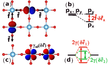
Figure 5: (Color online) Schematic representation of the effects of the expansion of $\gamma^{\text{sr}}$ in terms of atomic deformations. Panels (a) and (b) illustrate the electron-lattice coupling associated to diagonal, $\gamma_{\bm{a}\bm{a}}^{\text{sr}}$, matrix elements that control the average energy of the corresponding bands. In (a) we sketch the forces on the atoms (represented by red spheres) as generated by electrons placed on a $p_{x}$ or $p_{y}$-like WFs. In our method, these forces are captured by the tensor $\vec{f}$ in Eq. (62). In (b) we illustrate the change in the electronic structure as a consequence of the atomic displacement: if the atoms displace along $x$ in the way shown in the top atomic chain of panel (a), then a variation in the position of the $p_{x}$ orbitals is induced, while the $p_{y}$ level remains unaltered. Panels (c) and (d) illustrate the change in non-diagonal $\gamma^{\text{sr}}$ matrix elements between two neighboring orbitals when the intermediate atom moves, thus altering the band width as illustrated in (d). The change in the band width depends on the amount by which the atoms are displaced, represented in the cartoon by two different displacement vectors $\delta\vec{r}_{1}$ and $\delta\vec{r}_{2}$.

Finally, the geometrical dependence of the two-electron parameters, $U$ and $I$, can be included in our model in a similar way. Nevertheless, since these terms are not explicitly dependent on the potential created by the ions, their value can be expected to be less sensitive to changes in the atomic configuration. Hence, in this work, and in analogy to what is customarily done in model Hamiltonian and DFT+U approaches,Anisimov et al. (1997) we will neglect such effects.

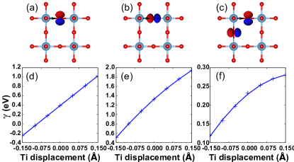
Figure 6: (Color online) Variation of the $\gamma$ matrix elements of bulk SrTiO₃ that are most sensitive to the the displacement of a Ti ion. Panels (a)-(c): the atoms at a TiO₂ plane are represented by big blue (Ti) and small red (O) spheres. The displacement of the Ti⁴⁺ is marked with an arrow. The Wannier-like functions related with the $\gamma$ matrix elements under consideration are plotted: (a) a $p$-like orbital with lobules pointing perpendicularly to the Ti⁴⁺ displacement ($\pi$-bonding), (b) a $p$-like orbital with lobules pointing parallel to the Ti⁴⁺ displacement ($\sigma$-bonding), and (c) two $p$-like orbitals centered on different O atoms with lobules pointing perpendicular in one case and parallel in the other to the Ti⁴⁺ displacement. In (a), and (b), the corresponding matrix element whose evolution is studied is diagonal (i.e., $\bm{a}=\bm{b}$), while in (c) the matrix element is off-diagonal ($\bm{a}\neq\bm{b}$). Panels (d)-(f) show the variation of these matrix elements with respect to the Ti displacement. First-principles results are represented by blue crosses, while the model values [see Eq. (62)] are represented by solid blue lines.

II.7 Total energy

Replacing the expressions for the one-electron [Eq. (21)], and two-electron [Eq. (39)] integrals into Eq. (5) for the total energy, we get

$$E= E^{(0)}+E^{(1)}+E^{(2)}$$

$$= E^{(0)}+\sum_{\bm{a}\bm{b}}D_{\bm{a}\bm{b}}^{U}\gamma_{\bm{a}\bm{b}}+$$

$$+\frac{1}{2}\sum_{\bm{a}\bm{b}}\sum_{\bm{a}^{\prime}\bm{b}^{\prime}}\left(D_{\bm{a}\bm{b}}^{U}D_{\bm{a}^{\prime}\bm{b}^{\prime}}^{U}U_{\bm{a}\bm{b}\bm{a}^{\prime}\bm{b}^{\prime}}-D_{\bm{a}\bm{b}}^{I}D_{\bm{a}^{\prime}\bm{b}^{\prime}}^{I}I_{\bm{a}\bm{b}\bm{a}^{\prime}\bm{b}^{\prime}}\right).$$ (65)

or, equivalently, in terms of the spin-up and spin-down densities,

$$E= E^{(0)}+\sum_{\bm{a}\bm{b}}\left(D_{\bm{a}\bm{b}}^{\uparrow}+D_{\bm{a}\bm{b}}^{\downarrow}\right)\gamma^{\text{sr}}_{\bm{a}\bm{b}}$$

$$+\frac{1}{2}\sum_{\bm{a}\bm{b}}\sum_{\bm{a}^{\prime}\bm{b}^{\prime}}\left\{\left(D_{\bm{a}\bm{b}}^{\uparrow}+D_{\bm{a}\bm{b}}^{\downarrow}\right)\left(D_{\bm{a}^{\prime}\bm{b}^{\prime}}^{\uparrow}+D_{\bm{a}^{\prime}\bm{b}^{\prime}}^{\downarrow}\right)\right.U_{\bm{a}\bm{b}\bm{a}^{\prime}\bm{b}^{\prime}}$$

$$\left.-\left(D_{\bm{a}\bm{b}}^{\uparrow}-D_{\bm{a}\bm{b}}^{\downarrow}\right)\left(D_{\bm{a}^{\prime}\bm{b}^{\prime}}^{\uparrow}-D_{\bm{a}^{\prime}\bm{b}^{\prime}}^{\downarrow}\right)I_{\bm{a}\bm{b}\bm{a}^{\prime}\bm{b}^{\prime}}\right\}$$ (66)

Now we introduce the decomposition of the $\gamma$ [Eqs. (57) and (58)] and $U$ [Eqs. (59) and (60)] parameters into long and short-range parts, and gather together all the long-range terms, to obtain,

$$E= E^{(0)}+\sum_{\bm{a}\bm{b}}D_{\bm{a}\bm{b}}^{U}\gamma^{\text{sr}}_{\bm{a}\bm{b}}$$

$$+\frac{1}{2}\sum_{\bm{a}\bm{b}}\sum_{\bm{a}^{\prime}\bm{b}^{\prime}}\left(D_{\bm{a}\bm{b}}^{U}D_{\bm{a}^{\prime}\bm{b}^{\prime}}^{U}U^{\text{sr}}_{\bm{a}\bm{b}\bm{a}^{\prime}\bm{b}^{\prime}}-D_{\bm{a}\bm{b}}^{I}D_{\bm{a}^{\prime}\bm{b}^{\prime}}^{I}I_{\bm{a}\bm{b}\bm{a}^{\prime}\bm{b}^{\prime}}\right)$$

$$+\sum_{\bm{a}}D_{\bm{a}\bm{a}}^{U}\left(-v_{\rm FF}(\vec{r}_{\bm{a}})+\frac{1}{2}\sum_{\bm{a}^{\prime}}D_{\bm{a}^{\prime}\bm{a}^{\prime}}^{U}U^{\text{lr}}_{\bm{a}\bm{a}\bm{a}^{\prime}\bm{a}^{\prime}}.\right)$$ (67)

Note that for the case of a non-spin polarized system ($D_{\bm{a}\bm{b}}^{I}=0$) the expression for the total energy reduces to

$$E= E^{(0)}+\sum_{\bm{a}\bm{b}}D_{\bm{a}\bm{b}}^{U}\gamma^{\text{sr}}_{\bm{a}\bm{b}}$$

$$+\frac{1}{2}\sum_{\bm{a}\bm{b}}\sum_{\bm{a}^{\prime}\bm{b}^{\prime}}D_{\bm{a}\bm{b}}^{U}D_{\bm{a}^{\prime}\bm{b}^{\prime}}^{U}U^{\text{sr}}_{\bm{a}\bm{b}\bm{a}^{\prime}\bm{b}^{\prime}}$$

$$+\sum_{\bm{a}}D_{\bm{a}\bm{a}}^{U}\left(-v_{\rm FF}(\vec{r}_{\bm{a}})+\frac{1}{2}\sum_{\bm{a}^{\prime}}D_{\bm{a^{\prime}}\bm{a}^{\prime}}^{U}U^{\text{lr}}_{\bm{a}\bm{a}\bm{a}^{\prime}\bm{a}^{\prime}}\right).$$ (68)

II.8 Self-consistent equations

As it is clearly seen in Eq. (67), the total energy in our formalism depends on the deformation occupation matrix defined in Eq. (19), and later generalized for the case of spin-polarized systems in Eqs. (30) and (31). This quantity is directly related with the deformation charge density, i.e., with the difference between the total charge density and the reference electronic density. It can be computed from the coefficients of the Bloch wave functions in the basis of Wannier functions, which are thus the only variational parameters of the method.

Solving for the ground state amounts to finding a point at which the energy is stationary upon variations in the electronic density, $n(\vec{r})$. Following a textbook procedure,Parr and Yang (1994); Jensen (1999); Martin (2004); Kohanoff (2006) we obtain a set of self-consistent conditions analogous to the Kohn-Sham equationsKohn and Sham (1965)

$$\sum_{b}h_{ab,\vec{k}}^{s}\,c_{jb\vec{k}}^{s}=\varepsilon_{j\vec{k}}^{s}\,c_{ja\vec{k}}^{s},$$ (69)

where, as defined above, $\varepsilon_{j\vec{k}}^{s}$, is the $j$-th band energy at wavevector $\vec{k}$ for the spin channel $s$. The corresponding Hamiltonian matrix, $h_{ab,\vec{k}}^{s}$, is

$$h_{ab,\vec{k}}^{s}=\sum_{\vec{R}_{B}-\vec{R}_{A}}e^{i\vec{k}\cdot\left(\vec{R}_{B}-\vec{R}_{A}\right)}h_{\bm{a}\bm{b}}^{s},$$ (70)

where $h_{\bm{a}\bm{b}}^{s}$ is the real-space Hamiltonian

$$h_{\bm{a}\bm{b}}^{s}=\gamma_{\bm{a}\bm{b}}+\sum_{\bm{a^{\prime}b}^{\prime}} \left[\left(D_{\bm{a}^{\prime}\bm{b}^{\prime}}^{s}+D_{\bm{a}^{\prime}\bm{b}^{\prime}}^{-s}\right)U_{\bm{aba^{\prime}b}^{\prime}}-\right.$$

$$\left.\left(D_{\bm{a}^{\prime}\bm{b}^{\prime}}^{s}-D_{\bm{a}^{\prime}\bm{b}^{\prime}}^{-s}\right)I_{\bm{aba^{\prime}b}^{\prime}}\right].$$ (71)

Note that this is a mean-field problem fully equivalent to that of the Hartree-Fock approach, and it must be solved self-consistently. The practical procedure for finding the solution is straightforward: given an initial guess for the deformation occupation matrix ($D_{\bm{a}\bm{b}}^{s}$), we compute the corresponding mean-field Hamiltonian ($h_{\bm{a}\bm{b}}^{s}$); from the diagonalization of this matrix we obtain a new deformation occupation matrix, and the procedure is iterated until reaching self-consistency. Note that electrostatic effects are accounted for by computing the long-range part of the $\gamma$ and $U$ parameters; this is our scheme’s equivalent to solving Poisson’s equation, as customarily done in DFT and other approaches.

Finally, note that in cases in which the system does not present any electron excitation – i.e., whenever the full density is equal to the reference density and we have $D_{\bm{a}\bm{b}}^{s}=0$ –, no self-consistent procedure is needed to obtain the solution.

II.9 Forces and stresses

Forces and stresses can be computed by direct derivation of the total energy [Eq. (65)] with respect to the atomic positions and cell strains. After some algebra, the result for the forces is,

$$\vec{F}_{\bm{\lambda}}=-\vec{\nabla}_{\bm{\lambda}}E=-\vec{\nabla}_{\bm{\lambda}}E^{(0)}-\sum_{\bm{a}\bm{b}}D_{\bm{a}\bm{b}}^{U}\vec{\nabla}_{\bm{\lambda}}\gamma_{\bm{a}\bm{b}},$$ (72)

where $\bm{\lambda}$ denotes a specific atom in a certain cell; here we assume that electron-lattice couplings are restricted to the one-electron terms.

The derivative of $E^{(0)}$ can be computed directly and exactly from the force-field on which our model is based.

The deformation occupation matrix $D_{\bm{a}\bm{b}}^{U}$ depends on the eigenvector coefficients and occupations. However, its derivative with respect to the atomic displacement is not required, since the energy is stationary with respect to these coefficients and occupations on the Born-Oppenheimer surface, and the Hellman-Feynman theorem guarantees that their first-order variation will not modify the total energy, and therefore will not affect the forces. Moreover, due to the orthogonality of the basis set used, no orthogonality forces need to be included, as it is the case when using a basis of non-orthogonal atomic orbitals (see Appendix A of Ref. Soler et al., 2002).

It is interesting to further inspect the similarity between the second term in our forces and the Hellmann-Feynman result,Martin (2004)

$$\vec{F}_{\bm{\lambda}}=-\vec{\nabla}E_{nn}-\sum_{j\vec{k}}o_{j\vec{k}}\left\langle\psi_{j\vec{k}}\right|\vec{\nabla}_{\bm{\lambda}}\hat{h}_{0}\left|\psi_{j\vec{k}}\right\rangle,$$ (73)

as (via a Fourier transform) $\vec{\nabla}_{\bm{\lambda}}\gamma_{\bm{a}\bm{b}}$ is analogous to $\langle\psi_{j\vec{k}}|\vec{\nabla}_{\bm{\lambda}}\hat{h}_{0}|\psi_{j\vec{k}}\rangle$, and $D_{\bm{a}\bm{b}}^{U}$ plays the role of the occupations $o_{j\vec{k}}$. This connection should be considered with caution, though, as our forces have a dominant contribution from the RED state, which is also included in the Hellmann-Feynman expression.

It is also interesting to note that, if we included the dependence of $U$ (and $I$) on the nuclear positions, we would have a Pulay term in Eq. (72),Pulay (1969) reflecting the change of the WF basis set with the atomic displacements.

Now we calculate the stress tensor in an analogous way. We adopt the standard definitionMartin (2004)

$$S_{\alpha\beta}=-\frac{1}{V}\frac{\partial^{\prime}E}{\partial^{\prime}\eta_{\alpha\beta}},$$ (74)

where $V$ is the volume of the real-space cell and $\partial^{\prime}$ denotes derivative keeping the fractional coordinates of the atoms in the system constant. We notice that there are only three terms in the energy that depend explicitly on the strain tensor $\overleftrightarrow{\eta}$, namely, the RED energy $E^{(0)}$, the short-range one-electron term, $\gamma_{\bm{a}\bm{b}}^{\text{sr}}$, and the electrostatic energy. Thus, we have

$$S_{\alpha\beta}=-\frac{1}{V}\left[\frac{\partial^{\prime}E^{(0)}}{\partial^{\prime}\eta_{\alpha\beta}}+\sum_{\bm{a}\bm{b}}D_{\bm{a}\bm{b}}^{U}\frac{\partial^{\prime}\gamma^{\text{s}r}_{\bm{a}\bm{b}}}{\partial^{\prime}\eta_{\alpha\beta}}+\frac{\partial^{\prime}E^{\text{elec}}}{\partial^{\prime}\eta_{\alpha\beta}}\right],$$ (75)

where $E^{\text{elec}}$ corresponds with the electrostatic energy as written in the fourth contribution to the total energy in Eq. (67). As in the case of the forces, the $E^{(0)}$ derivative is computed from the force field that describes the RED state. Similarly, the calculation of the last, electrostatic term can be achieved via Ewald summation techniques (see e.g. Ref. Kawata et al., 2001). The only term that requires further manipulation is the derivative of $\gamma_{\bm{a}\bm{b}}^{\text{sr}}$, Eq. (62), with respect to the strain, which yields

$$\frac{\partial^{\prime}\gamma_{\bm{a}\bm{b}}^{\text{sr}}}{\partial^{\prime}\eta_{\alpha\beta}}= \sum_{\bm{\lambda}\bm{\upsilon}}\left[-\vec{f}_{\bm{a}\bm{b},\bm{\lambda}\bm{\upsilon}}^{T}\frac{\partial^{\prime}\left(\delta\vec{r}_{\bm{\lambda}\bm{\upsilon}}\right)}{\partial^{\prime}\eta_{\alpha\beta}}+\right.$$

$$+\left.\sum_{\bm{\lambda}^{\prime}\bm{\upsilon}^{\prime}}\frac{\partial^{\prime}\left(\delta\vec{r}_{\bm{\lambda}\bm{\upsilon}}^{T}\right)}{\partial^{\prime}\eta_{\alpha\beta}}\left(\overleftrightarrow{g}\right)_{\bm{a}\bm{b},\bm{\lambda}\bm{\upsilon}\bm{\lambda}^{\prime}\bm{\upsilon}^{\prime}}\delta\vec{r}_{\bm{\lambda}^{\prime}\bm{\upsilon}^{\prime}}+\right.$$

$$+\left.\sum_{\bm{\lambda}^{\prime}\bm{\upsilon}^{\prime}}\delta\vec{r}_{\bm{\lambda}\bm{\upsilon}}^{T}\left(\overleftrightarrow{g}\right)_{\bm{a}\bm{b},\bm{\lambda}\bm{\upsilon}\bm{\lambda}^{\prime}\bm{\upsilon}^{\prime}}\frac{\partial^{\prime}\left(\delta\vec{r}_{\bm{\lambda}^{\prime}\bm{\upsilon}^{\prime}}\right)}{\partial^{\prime}\eta_{\alpha\beta}}\right].$$ (76)

As in the case of the forces, the similarity between this result and the Hellmann-Feynman expression is apparent.

To end this section, let us stress that only excited electrons/holes, which render $D_{\bm{a}\bm{b}}\neq 0$, create forces and stresses not included in the underlying force-field described by $E^{(0)}$. In fact, in the typical case, the dominant contribution to both forces and stresses will come from the derivative of $E^{(0)}$, with corrections that are linear in the difference occupation matrix.

II.10 Practical considerations

So far we have introduced a method for the simulation of materials at a large scale. We have presented the basic physical ingredients (reference atomic geometry, reference electronic density, deformation density, etc.), that allow us to approximate the DFT total energy, forces and stresses.

In this section we discuss some practicalities involved in the implementation of this method in a computer code to perform actual calculations. Of course, different implementations are in principle possible; here we briefly describe some details pertaining to our specific choices, which should be illustrative of the technical issues that need to be tackled.

II.10.1 Definition of the RED

The formulation above is written in terms of differences between the actual and reference states of the system in a completely general way. However, from a practical point of view, an appropriate choice of the RED, $n_{0}(\vec{r})$, is a necessary first step towards an efficient implementation of our method.

The most important ingredient to define $n_{0}$ is the reference occupation matrix that, following Eq. (17), amounts to

$$d_{\bm{a}\bm{b}}^{(0)}=\sum_{j\vec{k}}o_{j\vec{k}}^{(0)}\left[c_{ja\vec{k}}^{(0)}\right]^{*}c_{jb\vec{k}}^{(0)}e^{i\vec{k}(\vec{R}_{B}-\vec{R}_{A})},$$ (77)

where $o_{j\vec{k}}^{(0)}$ and $c_{ja\vec{k}}^{(0)}$ characterize the RED. While it would be possible to use the $d_{\bm{a}\bm{b}}^{(0)}$ result computed from first principles to perform second-principles simulations, in the following we shall simplify this expression in order to obtain a more convenient form.

Note that the reference occupation matrix satisfies $d_{\bm{a}\bm{b}}^{(0)}=0$ for $\bm{a}$ and $\bm{b}$ belonging to different band manifolds. (By definition, if $\bm{a}$ and $\bm{b}$ belong to different bands, they cannot appear simultaneously in the expansion of a particular Bloch state [Eq. (14)], and the corresponding $d_{\bm{a}\bm{b}}^{(0)}$ [Eq. (77)] will vanish.) It is thus possible to rewrite Eq. (77) and split the sum over states in two, one over manifolds $\mathcal{J}$ and a second one over bands within a manifold.

After having established this property, we impose that all the bands $j$ that belong to the same manifold $\mathcal{J}$ have the same occupation in the RED

$$o_{j\vec{k}}^{(0)}=o_{\mathcal{J}}\omega_{\vec{k}}=\frac{o_{\mathcal{J}}}{N_{k}},$$ (78)

where $\omega_{\vec{k}}$ is the weight of each $\vec{k}$-point in the BZ. As we assume an homogeneous sampling in reciprocal space, $\omega_{\vec{k}}=N_{k}^{-1}$, where $N_{k}$ is the total number of points in our BZ mesh. Thus, for example, in a diamagnetic insulator [see Fig. 3(a)] (where the valence and conduction band always belong to different manifolds) we would choose the occupation for the reference states so that all the valence bands are fully occupied while all conduction bands are completely empty. In this way the reference electronic density for a diamagnetic insulator is simply the ground state density.

For metals [Fig. 3(b)], and magnetic insulators [Fig. 3(c)], where a disentanglement procedureSouza et al. (2001) has to be carried out to separate the desired bands from others with which they are hybridized in a given energy window, the choice is not so simple. In such cases we distribute all the electrons of the entangled bands equally among the bands in the manifold. For example, in the case of metallic copper [Fig. 3(b)], which has an electronic configuration 3$d^{10}$4$s^{1}$ where the five 3$d$ functions cross with the 4$s$-like band, we would distribute the eleven electrons over the six bands taking $o_{\mathcal{J}}=11/6$. On the other hand, for NiO [Fig. 3(c)] some Ni(3$d$) bands are occupied and entangled with the O(2$p$) ones; at the same time, empty $e_{g}$-like orbitals are part of the conduction band and entangled with other levels there. Here, we choose to disentangle the bands with strong Ni(3$d$) and O(2$p$) character from the other bands. Further, we assign the occupation by distributing the corresponding electrons – eight 3$d$ electrons of Ni²⁺ and the six 2$p$ electrons of O^2- – over the corresponding bands – five 3$d$ bands and three 2$p$ bands – yielding $o_{\mathcal{J}}=14/8$. Taking into account the spin polarization, the occupation per spin channel is just $o_{\mathcal{J}}=7/8$.

Using Eq. (78) to rewrite Eq. (77), and taking into account the relationship between the coefficients of RED Bloch states and the unitary transformations between Bloch and Wannier representations, we have

$$d_{\bm{a}\bm{b}}^{(0)} =N_{k}^{-1}o_{\mathcal{J}}\sum_{\vec{k}}e^{i\vec{k}(\vec{R}_{B}-\vec{R}_{A})}\sum_{j}\left[\left(T_{aj}^{(\vec{k})}\right)^{-1}\right]^{*}\left(T_{bj}^{(\vec{k})}\right)^{-1}$$

$$=N_{k}^{-1}o_{\mathcal{J}}\sum_{\vec{k}}e^{i\vec{k}(\vec{R}_{B}-\vec{R}_{A})}\sum_{j}T_{ja}^{(\vec{k})}\left(T_{bj}^{(\vec{k})}\right)^{-1}$$

$$=N_{k}^{-1}o_{\mathcal{J}}\sum_{\vec{k}}e^{i\vec{k}(\vec{R}_{B}-\vec{R}_{A})}\delta_{ab}$$

$$=N_{k}^{-1}o_{\mathcal{J}}\delta_{ab}\sum_{\vec{k}}e^{i\vec{k}(\vec{R}_{B}-\vec{R}_{A})}$$

$$=o_{\mathcal{J}}\delta_{ab}\delta_{\vec{R}_{A}\vec{R}_{B}}=o_{\mathcal{J}}\delta_{\bm{a}\bm{b}},$$ (79)

where we have used the properties of the unitary matrices. From this expression we see that $o_{\mathcal{J}}$ is simply the occupation of the WF $\chi_{\bm{a}}$ in the reference state, $o_{\bm{a}}^{(0)}$. Finally, inserting Eq. (79) into Eq. (18), we arrive to the conclusion that

$$n_{0}(\vec{r}) =\sum_{\bm{a}\bm{b}}d^{(0)}_{\bm{a}\bm{b}}\chi_{\bm{a}}(\vec{r})\chi_{\bm{b}}(\vec{r})$$

$$=\sum_{\bm{a}\bm{b}}o_{\mathcal{J}}\delta_{\bm{a}\bm{b}}\chi_{\bm{a}}(\vec{r})\chi_{\bm{b}}(\vec{r})$$

$$=\sum_{\bm{a}}o_{\mathcal{J}}|\chi_{\bm{a}}(\vec{r})|^{2}$$

$$=\sum_{\bm{a}}o_{\bm{a}}^{(0)}|\chi_{\bm{a}}(\vec{r})|^{2},$$ (80)

where we have used the fact that $o_{\bm{a}}^{(0)}=o_{\mathcal{J}}$ for all WFs in the manifold.

We would like to stress that this approach simply allows for a more efficient computational method since we can still retrieve the full electron distribution in space by substituting the first-principles WFs into Eqs. (16) and (18).

II.10.2 Deformation electron density

From the definition of the charge density in terms of the density matrix, Eq. (16), and the orthogonality of the Wannier basis functions, it trivially follows that the total number of electrons in the system is the trace of the density matrix,

$$N =\int n(\vec{r})d^{3}r=\int\sum_{\bm{a}\bm{b}}d_{\bm{a}\bm{b}}\chi_{\bm{a}}(\vec{r})\chi_{\bm{b}}(\vec{r})d^{3}r$$

$$=\sum_{\bm{a}\bm{b}}d_{\bm{a}\bm{b}}\int\chi_{\bm{a}}(\vec{r})\chi_{\bm{b}}(\vec{r})d^{3}r$$

$$=\sum_{\bm{a}\bm{b}}d_{\bm{a}\bm{b}}\delta_{\bm{a}\bm{b}}$$

$$=\sum_{\bm{a}}d_{\bm{a}\bm{a}}.$$ (81)

Therefore, the trace of the deformation matrix gives the number of extra electrons or holes that dope the system.

From the very definition of the deformation matrix, we can deduce that if its diagonal element,

$$D_{\bm{a}\bm{a}}=d_{\bm{a}\bm{a}}-d_{\bm{a}\bm{a}}^{(0)},$$ (82)

is negative (positive), that means that we are creating holes (inserting electrons) on that particular state, as illustrated in Fig. 1.

The fact that most of these electron/hole excitations take place around the Fermi energy has a very important consequence with regards to the efficiency of the method. In order to calculate $D_{\bm{a}\bm{a}}$, and the total energy [see Eq. (67)], we do not need to obtain all the eigenvalues of the one-electron Hamiltonian, but just those around the Fermi energy. This opens up the possibility to use efficient diagonalization techniques that allow a fast calculation of a few relevant eigenvalues, e.g. Lanczos. This approach allows us to speed up the calculations in a very significant manner. (The diagonalization of the full Hamiltonian matrix is one of the main computational bottlenecks in electronic structure methods.) Along these lines, the possibility of obtaining linear scaling within our method will be discussed in a future publication.

III Parameter calculation

The method presented above allows for the simulation of very large systems under operation conditions assuming that a few parameters describing one-electron and two-electron interactions, as well as the electron-lattice couplings, are known beforehand. For the sake of preserving predicting power, it is important to compute those parameters from first principles.

All the electronic parameters of our models have well-defined expressions [see Eq. (23) for $\gamma_{\bm{a}\bm{b}}$, Eq. (40) for $U_{\bm{a}\bm{b}\bm{a}^{\prime}\bm{b}^{\prime}}$ and Eq. (41) for $I_{\bm{a}\bm{b}\bm{a}^{\prime}\bm{b}^{\prime}}$], whose computation requires only the knowledge of the Wannier functions, the one-electron Hamiltonian, and the operators involved in the double integrals, all of them defined for the RED. Since the chosen basis functions are localized in space, the required calculations could be performed on small supercells. Such a direct approach to obtain the model parameters is thus, in principle, feasible.

Note that there has been significant work to calculate related integrals from first principles, as can be found e.g. in Refs. Marzari and Vanderbilt, 1997; Mostofi et al., 2008; Liechtenstein et al., 1995; Anisimov et al., 1997; Aryasetiawan and Gunnarsson, 1998; Anisimov and Gunnarsson, 1991; Solovyev, 2008; Solovyev and Imada, 2005; Gunnarsson et al., 1989; Miyake and Aryasetiawan, 2008; Nakamura et al., 2006; Vaugier et al., 2012. Yet, we feel that most of these approaches are too restrictive for the more general task that we pursue in this work. For instance, the focus in the previous references is placed on strongly correlated electrons in a single center, while we are also interested in multi-center integrals.

A significant effort would thus be required to implement the calculation of the more complex interactions, including all the potentially relevant ones, and developing tools to derive minimal models that retain only the dominant parameters and capture the main physical effects. Note that, in a typical system, the number of potentially relevant integrals will be very large. In fact, the presence of four-index integrals like $U_{\bm{a}\bm{b}\bm{a}^{\prime}\bm{b}^{\prime}}$ and $I_{\bm{a}\bm{b}\bm{a}^{\prime}\bm{b}^{\prime}}$ is the reason why Hartree-Fock schemes scale much worse than DFT methods with respect to the number of basis functions in the calculation [$\sim\mathcal{O}(N^{5})$ vs. $\sim\mathcal{O}(N^{3})$, respectively]. Hence, at the present stage we have not attempted a direct first-principles calculation of the parameters, which is a challenge that remains for the future. Instead, we have devised a practical scheme to fit our models to relevant first-principles data.

III.1 Parameter fitting

Our procedure comprises several steps.

Training set

First, we identify a training set (TS) of representative atomic and electronic configurations from which the relevant model parameters will be identified and computed. For example, the training set for a magnetic system should contain simulations for several spin arrangements, so that the mechanisms responsible for the magnetic couplings can be captured. Additionally, if we want to study a system whose bands are very sensitive to the atomic structure, the training set should contain calculations for different geometries so that this effect is captured. Alternatively, if we want to describe how doping affects the physical properties of a material, then different DFT simulations on charged systems should be carried out,Makov and Payne (1995) etc.

Let us note that it is typically possible to restrict the TS to atomic and electronic configurations compatible with small simulation boxes. This translates into (and is consistent with) the fact that, when expressed in a basis of localized WFs, the non-electrostatic interactions in most materials are short ranged.

We will use $N_{\rm TS}$ to denote the total number of TS elements, noting that we will run a single-point first-principles calculation for each of them. Further, $N_{\rm RAG}$ is the number of TS configurations that correspond to the reference atomic geometry.

Filtering the training set

Let $h_{\bm{a}\bm{b}}^{s}(i)$ be the Hamiltonian of the $i$-th TS configuration, in matrix form and as obtained from a first-principles (typically DFT) calculation. We denote the whole collection of one-electron Hamiltonians in the training set by $\{h_{\bm{a}\bm{b}}^{s}(i)\}$.

These Hamiltonians are expressed in a basis of localized WFs. Formally, they can be obtained by inverting Eq. (70) (see Sec. VI A of Ref. Marzari et al., 2012), so that

$$h_{\bm{a}\bm{b}}^{s}=\frac{(2\pi)^{3}}{V}\int_{\text{BZ}}d^{3}k\left[\sum_{j}\left[T_{ja}^{s(\vec{k})}\right]^{\star}\varepsilon_{j\vec{k}}^{s}T_{jb}^{s(\vec{k})}\right]e^{i\left(\vec{R}_{A}-\vec{R}_{B}\right)\vec{k}},$$ (83)

where the ${\bm{T}}$ matrices are unitary transformations that convert the first-principles eigenstates into Bloch-like waves associated to specific (localized) WFs. These transformations can be obtained by employing codes like wannier90,Mostofi et al. (2008) which implements a particular localization scheme, i.e., a particular way to compute optimum ${\bm{T}}$ matrices.Marzari and Vanderbilt (1997); Marzari et al. (2012)

Once the $h_{\bm{a}\bm{b}}^{s}(i)$ Hamiltonians are known, we can identify the pairs of WFs with a large enough interaction and which need to be retained in the fitting procedure. In practice, we introduce a cut-off energy $\delta\varepsilon_{h}$ such that

$$|h_{\bm{a}\bm{b}}^{s}(i)|>\delta\varepsilon_{h},\text{for at least one $i$ in the TS},$$ (84)

defines the Hamiltonian matrix elements to be retained. (Diagonal elements, $h_{\bm{a}\bm{a}}^{s}$, are always considered independently of their value.) This condition allows us to identify the WF pairs $(\bm{a}$, $\bm{b})$ to be included in the fitting procedure, regardless of the geometry or spin arrangement.

In Fig. 7 we compare the full first-principles bands for SrTiO₃ and NiO with those obtained from models corresponding to different energy cut-offs. For all the $\delta\varepsilon_{h}$ values considered, we also indicate the number of parameters in the resulting models. This allows us to estimate the size of the model (and associated computational cost) needed to achieve an acceptable description of the band structure.

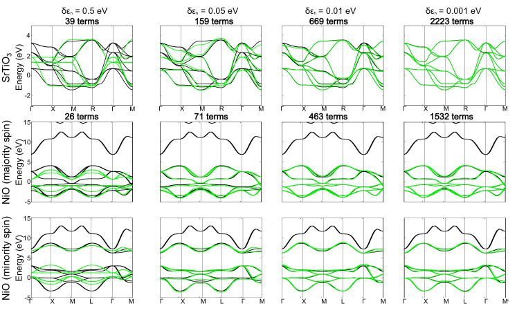
Figure 7: (Color online) Representation of the bands of SrTiO₃ (top row) and NiO (middle and bottom rows, corresponding to the majority and minority spin channels, respectively) for various values of the Hamiltonian cutoff, $\delta\varepsilon_{h}$. Black lines represent the bands as obtained from first principles, while the results from the second-principles model are shown in green. On top of each plot we indicate the corresponding number of $h_{\bm{a}\bm{b}}^{s}$ matrix elements per primitive cell that were included.

Identifying most relevant model interactions

Our models, even though we truncate them at second order of the expansion in Eq. (5), contain a daunting number of electron-electron interaction parameters. Constructing an actual model usually involves further approximations regarding the spatial range of the interactions, the maximum number of different bodies (WFs) involved, etc. Hence, we need a procedure to identify the simplest models that can reproduce the first-principles TS data with an accuracy that is sufficient for our purposes.

The scheme we have implemented is based on a very simple logic: We start from a certain complete model that may contain, in principle, all possible one-electron, two-electron, and electron-lattice parameters. We can then fit such a model to reproduce the one-electron Hamiltonians $\{h_{\bm{a}\bm{b}}^{s}(i)\}$ of our TS within a certain accuracy. Typically, by doing so, and by systematically exploring different combinations of parameters in the model, we can identify the simplest interactions (i.e., those that are shortest in range, involve fewest WFs, etc.) sufficient to achieve the desired level of accuracy; in other words, in this way we can identify non-critical couplings that just render the fitting problem underdetermined, do not improve the accuracy of the model, and can thus be disregarded. Naturally, this split between relevant and irrelevant couplings is strongly dependent on the choice of the training set, which should be complete enough to capture the physical effects of interest.

To better understand how the scheme works, consider the one-electron integrals $\gamma_{\bm{a}\bm{b}}$ in the case of a non-magnetic material like SrTiO₃. These parameters will be the only ones entering the description of the band structure of the RAG in the RED state. Hence, we can fit them directly by requiring our model to reproduce the Hamiltonian $h_{\bm{a}\bm{b}}$ of this particular, reference state with a certain accuracy.

More generally, the one-electron Hamiltonian corresponding to a TS configuration will reflect electronic excitations departing from the RED state. More precisely, we can recall Eq. (71) to write

$$h_{\bm{a}\bm{b}}^{s}(i)=\gamma_{\bm{a}\bm{b}}+\sum_{\bm{a^{\prime}b}^{\prime}} \left[\left(D_{\bm{a}^{\prime}\bm{b}^{\prime}}^{s}(i)+D_{\bm{a}^{\prime}\bm{b}^{\prime}}^{-s}(i)\right)U_{\bm{aba^{\prime}b}^{\prime}}-\right.$$

$$\left.\left(D_{\bm{a}^{\prime}\bm{b}^{\prime}}^{s}(i)-D_{\bm{a}^{\prime}\bm{b}^{\prime}}^{-s}(i)\right)I_{\bm{aba^{\prime}b}^{\prime}}\right],$$ (85)

where we restrict ourselves to TS configurations at the RAG, so that no electron-lattice term appears in this equation. It is convenient to isolate the $U$ contribution by defining

$$h_{\bm{a}\bm{b}}^{U}(i)=\frac{h_{\bm{a}\bm{b}}^{\uparrow}(i)+h_{\bm{a}\bm{b}}^{\downarrow}(i)}{2}=\gamma_{\bm{a}\bm{b}}+\sum_{\bm{a^{\prime}b}^{\prime}}D_{\bm{a}^{\prime}\bm{b}^{\prime}}^{U}(i)U_{\bm{aba^{\prime}b}^{\prime}},$$ (86)

and its average over all the RAG configurations in the training set,

$$\bar{h}_{\bm{a}\bm{b}}^{U}=\frac{1}{N_{\rm RAG}}\sum_{i}h_{\bm{a}\bm{b}}^{U}(i)=\gamma_{\bm{a}\bm{b}}+\sum_{\bm{a^{\prime}b}^{\prime}}\bar{D}_{\bm{a}^{\prime}\bm{b}^{\prime}}^{U}U_{\bm{aba^{\prime}b}^{\prime}}.$$ (87)

Analogously, the antisymmetrization of the Hamiltonian matrix elements with respect to the spin yields

$$h_{\bm{a}\bm{b}}^{I}(i)=\frac{h_{\bm{a}\bm{b}}^{\uparrow}(i)-h_{\bm{a}\bm{b}}^{\downarrow}(i)}{2}=\sum_{\bm{a^{\prime}b}^{\prime}}D_{\bm{a}^{\prime}\bm{b}^{\prime}}^{I}(i)I_{\bm{aba^{\prime}b}^{\prime}}.$$ (88)

We expect that the most important $U_{\bm{a}\bm{ba^{\prime}b}^{\prime}}$ and $I_{\bm{a}\bm{ba^{\prime}b}^{\prime}}$ parameters will be, respectively, those involving WF pairs whose corresponding $h_{\bm{a}\bm{b}}^{U}(i)$ and $h_{\bm{a}\bm{b}}^{I}(i)$ are most strongly dependent on the TS state. Hence, we introduce the two-electron cutoff energy, $\delta\varepsilon_{ee}$, and retain only the $(\bm{a},\bm{b})$ pairs that satisfy, for at least one TS configuration, at least one of the following conditions:

$$|h_{\bm{a}\bm{b}}^{U}(i)-\bar{h}_{\bm{a}\bm{b}}^{U}|=\left|\sum_{\bm{a^{\prime}b}^{\prime}}\left[D_{\bm{a}^{\prime}\bm{b}^{\prime}}^{U}(i)-\bar{D}_{\bm{a}^{\prime}\bm{b}^{\prime}}^{U}\right]U_{\bm{aba^{\prime}b}^{\prime}}\right|>\delta\varepsilon_{\text{ee}},$$ (89)

or

$$|h_{\bm{a}\bm{b}}^{I}(i)|=\left|\sum_{\bm{a^{\prime}b}^{\prime}}D_{\bm{a}^{\prime}\bm{b}^{\prime}}^{I}(i)I_{\bm{aba^{\prime}b}^{\prime}}\right|>\delta\varepsilon_{\text{ee}}.$$ (90)

Note that we gauge the $h_{\bm{a}\bm{b}}^{U}$ matrix elements with respect to the $\bar{h}_{\bm{a}\bm{b}}^{U}$ average values so that the corresponding cut-off condition does not depend on the one-electron couplings $\gamma$.

Once we have selected all the $\{(\bm{a},\bm{b})\}$ pairs that fulfill such criteria, we can build the list of potentially relevant $U$ and $I$ constants to be considered in the fit. Note that the number of free parameters is usually reduced by the fact that the $U_{\bm{a}\bm{b}\bm{a}^{\prime}\bm{b}^{\prime}}$ and $I_{\bm{a}\bm{b}\bm{a}^{\prime}\bm{b}^{\prime}}$ integrals are invariant upon permutations of the $(\bm{a},\bm{b},\bm{a}^{\prime},\bm{b}^{\prime})$ indexes. In some cases, and in spite of the reduction of parameters due to symmetry, the list of relevant interactions is excessively long and needs to be further trimmed to successfully carry out the fitting. In such situations we introduce a third cutoff, $\delta D$, that operates over the difference occupation matrix to select the interactions associated to important changes of the electron density. When doing so we only accept $U$ constants for which at least one pair of the associated indexes fulfills

$$|D_{\bm{a^{\prime}b}^{\prime}}^{U}(i)-\bar{D}_{\bm{a^{\prime}b}^{\prime}}^{U}|>\delta D$$ (91)

and the corresponding expression for $I$

$$|D_{\bm{a^{\prime}b}^{\prime}}^{I}(i)|>\delta D.$$ (92)

Let us also note that the most relevant $\gamma_{\bm{a}\bm{b}}$ parameters are trivially identified when we filter the TS one-electron Hamiltonians as described above.

Fitting the RAG model

Once our list of relevant $\gamma$, $U$, and $I$ parameters is complete, we fit them to reproduce the $\{h^{s}_{\bm{a}\bm{b}}\}$ matrix elements above the $\delta\varepsilon_{h}$ energy cutoff introduced previously.

We have found it convenient to perform the fit in several steps, so that different types of parameters are computed separately. More precisely, we first fit the $U$ parameters by requesting that our model reproduces the $h_{\bm{a}\bm{b}}^{U}(i)-\bar{h}_{\bm{a}\bm{b}}^{U}$ matrices [Eqs. (86) and (87)]. Analogously, we obtain the $I$ constants by fitting to the $h_{\bm{a}\bm{b}}^{I}(i)$ matrices [Eq. (88)]. Importantly, both of these fits are independent of the one-electron integrals, and have typically yielded well-posed, overdetermined systems of equations in the cases we have so far considered. Finally, we obtain the $\gamma$ parameters from the fitted $U$’s directly from Eq. (86). Direct comparison of the modeled bands with those obtained from the full first-principles $\{h^{s}_{\bm{a}\bm{b}}(i)\}$ set provides an estimate of the goodness of the model (see the example in Section V.2 and, particularly, Fig. 9).

Note that, alternatively, one could try a direct fit of all the $\gamma$, $U$, and $I$ parameters to the real-space Hamiltonians, using Eq. (71). However, we typically find that this strategy leads to nearly-singular problems in which very different solutions lead to comparably good results. In the general case, such a difficulty may be mitigated by extending the TS. However, here we adopted the simple and practical procedure described above, which permits a numerically stable method that yields accurate and physically sound models.

To end with this section we would like to stress that the $\gamma_{\bm{a}\bm{b}}$ constants obtained with this procedure contain both the short- and long-range contributions described above [Eq. (58)]. In order to isolate $\gamma^{\text{sr}}_{\bm{a}\bm{b}}$, we simply subtract the corresponding electrostatic contribution [Eq. (57)] from the determined, full $\gamma_{\bm{a}\bm{b}}$ value. In order to calculate the electrostatic contribution [Eqs. (55)-(56)] we need first-principles results for the Born charge tensor, $\overleftrightarrow{Z}_{\bm{\lambda}}^{*}$, and the high-frequency dielectric tensor, $\overleftrightarrow{\epsilon_{\infty}}$, that can routinely be obtained for systems where the RED is insulating. Note (1)

Relevant electron-lattice interactions

As above, we assume that the deviations from the RAG only affect the one-electron integrals $\gamma$, and not the $U$ and $I$ parameters. We further assume that such a dependence on the atomic structure is given by the linear and quadratic electron-lattice constants $\vec{\bm{f}}$ and $\overleftrightarrow{\bm{g}}$ introduced in Eq. (62).

The selection of the most important electron-lattice couplings is performed by observing how much a particular matrix element $h^{s}_{\bm{a}\bm{b}}$ changes with a particular distortion of the lattice with respect to the RAG. To quantify this change, we need to compare pairs of configurations $i$ and $i^{\prime}$ that correspond to the same electronic state (e.g., to the same spin arrangement, to the same amount of electron/hole doping, etc.) but differ in their atomic structure. More precisely, one of the configurations must correspond to the RAG state ($i$), while the other one ($i^{\prime}$) is characterized by a distortion given by $\{\vec{u}_{\bm{\lambda}}(i^{\prime})\}$. For simplicity, here we will restrict to distortions involving only one displacement component of one atom, so that we only have one specific $u_{{\bm{\lambda}}\alpha}(i^{\prime})\neq 0$, where $\alpha$ labels the spatial direction. We then consider that a particular atom $\bm{\lambda}$ participates in the electron-lattice affecting the $h_{\bm{a}\bm{b}}^{s}$ element if

$$\frac{1}{|u_{{\bm{\lambda}}\alpha}|}\left|h_{\bm{a}\bm{b}}^{s}(i^{\prime})-h_{\bm{a}\bm{b}}^{s}(i)\right|>\delta f_{e-l},$$ (93)

where $\delta f_{e-l}$ is a new cut-off. Note that, for a large enough distortion $|u_{{\bm{\lambda}}\alpha}|$, this condition pertains to both the linear ($\vec{\bm{f}}$) and quadratic ($\overleftrightarrow{\bm{g}}$) electron-lattice interactions. Yet, since we activate a single atomic displacement at a time, in the case of $\overleftrightarrow{\bm{g}}$ we are only probing the diagonal elements. Restricting ourselves to the diagonal elements of $\overleftrightarrow{\bm{g}}$ is justified by the observation that, in the systems we have so far studied, those are the only significant ones. At any rate, the scheme can be trivially extended to check a possible contribution of off-diagonal terms.

IV Implementation of the algorithm: The scale-up code

We have implemented this new method in the scale-up (Second-principles Computational Approach for Lattice and Electrons) package, written in Fortran 90 and parallelized using Message Passing Interface (MPI). Presently, this code can perform single-point calculations, geometry optimizations, and Born-Oppenheimer molecular dynamics using either full diagonalization or the Lanczos scheme mentioned above.

The energy of the reference state, $E^{(0)}$, is obtained from model potentials like those introduced by Wojdeł et al.,Wojdeł et al. (2013) which are interfaced with scale-up. We have also developed an auxiliary toolbox (modelmaker) for the calculation of all the parameters defining $E^{(1)}$ and $E^{(2)}$, using as input DFT results for one-electron Hamiltonians in the format of wannier90.Mostofi et al. (2008) As shown in Sec. V, these implementations can be used to create models that match the accuracy of the DFT calculations at an enormously reduced computational cost, opening the door to large-scale simulations (up to tens of thousands of atoms) of systems with a complex electronic structure, using modest computational resources.

The input to the code is based on the flexible data format (fdf) library used in siestaSoler et al. (2002) and contains several python-based tools to plot bands, density of states, geometries and other properties.

V Examples of application

In order to illustrate the method, we will discuss its application to two non-trivial systems with interactions of very different origin.

The first example consists in the calculation of the energy of a Mott-Hubbard insulator, NiO, for different magnetic phases. Our goal here is to show that the method can be used to deal accurately with complicated electronic structures including phenomena like magnetism in transition metal oxides. In this example we will also show how the method can tackle rather large systems (2,000 atoms) that are at the limit of what can be done with first-principles methods today, reducing the computational burden by orders of magnitude.

The second application involves the two-dimensional electron gas (2DEG) that appears at the interface between band insulators LaAlO₃ and SrTiO₃. Ohtomo and Hwang (2004) We will not discuss here the origin of the 2DEG, which has been treated in great detail in the bibliography.Ohtomo and Hwang (2004); Nakagawa et al. (2006); Stengel (2011); Bristowe et al. (2014) Rather, we will check whether our approach can predict the redistribution of the conduction electrons at the LaAlO₃/SrTiO₃ interface, and the accompanying lattice distortion, as obtained from first principles. Thus, this example will showcase the treatment of electron-lattice couplings and electrostatics within our approach.

V.1 Details of the first-principles simulations

We construct our models following the recipes described in Sec. III, and the first-principles data are obtained from small-scale calculations with the VASP package.Kresse and Fürthmuller (1996); Kresse and Joubert (1999); Blöchl (1994) The local density approximation (LDA) to density-functional theory is used to create the TS data for SrTiO₃. The calculations for NiO are also based on the LDA, but in this case an extra Hubbard-$U$ term is included to account for the strong electron correlations,Dudarev et al. (1998) as will be discussed below. We employ the projector-augmented wave (PAW) schemeBlöchl (1994) to treat the atomic cores, solving explicitly for the following electrons: Ni’s $3s$, $3p$, $3d$, and $4s$; O’s $2s$ and $2p$; Sr’s $3s$, $3p$, and $4s$; and Ti’s $3s$, $3p$, $3d$, and $4s$. The electronic wave functions are described with a plane-wave basis truncated at 300 eV for NiO and at 400 eV for SrTiO₃. The integrals in reciprocal space are carried out using $\Gamma$-centered 4$\times$4$\times$4 $k$-point meshes in both cases.

V.2 NiO magnetic couplings

Transition metal oxides are very interesting as they present optical, magnetic, and structural properties that are, very often, tightly coupled with each other. This fact, together with the large variety of functional properties that they can display, makes them a big focus of attention in both basic and applied materials science. From a theoretical point of view their study is complicated, mostly because of the strong correlations associated to the electrons in the compact $d$ shell (especially, those of first-row 3$d$ transition metal ions) and the frequent presence of many competing magnetic phases. Naively, one may expect most of these oxides to be metallic due to their open-shell nature while, in fact, many are insulators. This problem strongly affects computational methods; in fact, most common approaches, like DFT with local or semilocal exchange-correlation functionals, often fail to correctly reproduce the magnetic or insulating properties of these compounds. Simulations at this level of theory yield too diffuse states with underestimated interactions. The key to simulate successfully these materials lies in the way electron-electron interactions are handled. A panoply of methods have been developed to deal with this issue from first principles, ranging from the inclusion of a Hubbard-like term in the Hamiltonian in the so-called DFT+U methods, to more sophisticated schemes with dynamically screened interactions, such as the GW approximations.Hedin (1965); Aryasetiawan and Gunnarsson (1998)

For this first application of our scheme, we have chosen a simple transition metal oxide, NiO, a staple example of many new electronic structure simulation methods. Our goal is to show how our second-principles scheme can handily be used to compute the properties of strongly correlated materials, based on parameters obtained from first-principles LDA+U simulations. In particular we will study the band structure and magnetism of this archetypical binary oxide.

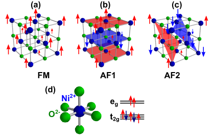
Figure 8: (Color online) Schematic cartoon of different magnetic configurations of bulk NiO in the conventional cell of its rocksalt structure: (a) ferromagnetic phase (FM), (b) antiferrognatic phase with planes of spin-up (red arrows) and spin-down (blue arrows) polarized nickels alternating along the $[001]$ direction (AF1), and (c) antiferrognatic phase with planes of spin-up and spin-down polarized nickels alternating along the $[111]$ direction (AF2). (d) Scheme of the $d$-levels associated to an isolated NiO${}_{6}^{10-}$ complex.

V.2.1 Parameters

The geometric structure of NiO shows some subtle and not fully understood distortions associated to its magnetism,Cheetham and Hope (1983); Schrön et al. (2012) but this issue is beyond the scope of the present work. In order to keep the model as simple and illustrative as possible, we neglect the lattice degrees of freedom in this case. As regards the spin order, neutron diffraction experimentsRoth (1958) show that the ground state corresponds to the so-called AF2 phase, where planes of spin-up and spin-down polarized nickels alternate along the $\left\langle 111\right\rangle$ direction of the conventional cell [see Fig. 8(c)]. Further experimentsSrinivasan and Seehra (1983); Chatterji et al. (2009) evidence that the AF2 to paramagnetic transition is of second order and occurs at a Nèel temperature $T_{N}$ = 524 K.

The simulations of NiO are carried out in the experimental rocksalt cell, with a lattice constant of 4.17 Å.Schmahl et al. (1964) This cell is compatible with several spin arrangements ranging from fully ferromagnetic [FM; Fig. 8(a)] to various antiferromagnetic (AF) ones [Fig. 8(b)-(c)]. Our TS includes the ground state spin arrangement (AF2) as well as the ferromagnetic one, which we choose because it represents a relevant limit case for spin–spin interactions. We use the LDA+U approach introduced by Dudarev et al.,Dudarev et al. (1998) with an effective U value of 7 eV, applied only on the 3$d$ orbitals of Ni. These calculations indicate that the AF2 solution is more stable than the FM one by 89 meV per formula unit (f.u.).

Ligand-field theory predicts the magnetism in this lattice to be the result of the half-filled $e_{g}$ shell of the octahedrally coordinated Ni²⁺ ion [see Fig. 8(d)]. Thus, we expect the levels around the Fermi energy to have this character. After calculating the electronic structure from first principles within the LDA+U, we find that the top valence and bottom conduction bands are composed of several strongly entangled states, as shown in Fig. 3(c). Thus, we project our WFs seeking to disentangle orbitals participating in the valence band [Ni($t_{2g}$), Ni($e_{g}$), and O($p$)] from others in the conduction band; to do this we use the tools provided within the wannier90 package. A graphical representation of the resulting orbitals [Fig. 3(c)] clearly shows that we are able to isolate bands with the expected chemical character: the isosurfaces of the maximally-localized WFs (MLWFs) at the right hand side of Fig. 3(c) clearly resemble the shape of the O(${p}$), Ni($d_{xy}$), and Ni($d_{3z^{2}-r^{2}}$) orbitals for the valence band, and of the Ni($d_{3z^{2}-r^{2}}$) orbital for the bottom of the conduction band. Given the strong entanglement of these bands, we use a reference occupation for the construction of our model that is obtained by populating equally all of them. As discussed in Sec. II.10.1, this amounts to assuming $o_{\mathcal{J}}=7/8=0.875$ electrons per band and spin channel.

At this point we start with the analysis of the Hamiltonian as described in Sec. III, using the $\{h^{s}_{\bm{a}\bm{b}}(i)\}$ set obtained after the disentanglement procedure. First, we seek to choose a reasonable value of $\delta\varepsilon_{h}$ that allows us to describe accurately the system’s bands without including an excessive number of $\gamma_{\bm{a}\bm{b}}$ terms. As can be seen in Fig. 7, $\delta\varepsilon_{h}$ = 0.05 eV is a reasonable choice; this involves the use of 71 $\gamma$ terms per f.u.

In order to decide the values of $\delta\varepsilon_{ee}$ and $\delta D$ that will determine the $U$ and $I$ parameters considered in the fit, we first examine the occupation difference of each of the WFs, $D_{\bm{a}\bm{a}}$. Let us recall that the diagonal elements of the deformation occupation matrices are defined as the difference between the reduced density matrix computed at the LDA+U for the corresponding configuration in the TS and the reference one. In the FM phase, the bands with $e_{g}$ character for the majority spin channel are expected to be fully occupied ($d_{\bm{a}\bm{a}}$ = 1), while they should be empty for the minority spin ($d_{\bm{a}\bm{a}}$ = 0). Therefore, for WFs with $e_{g}$ character, we expect to have $D_{\bm{a}\bm{a}}$ = 0.125 for the majority spins and $D_{\bm{a}\bm{a}}$ = $-$0.875 for the minority spins, for both Ni atoms. For the antiferromagnetic configuration, as the spin in one of the Ni atoms is reversed, we expect the same behavior for $D_{\bm{a}\bm{a}}$ as in the FM solution for one of the nickels, while the character of the majority and minority spins must be exchanged for the second Ni. In both cases (FM and AF2), the $t_{2g}$ bands are fully occupied, so that the corresponding $D_{\bm{a}\bm{a}}$ should be 0.125. These tendencies are well reproduced in our TS configurations as can be seen in Table 1, where the occupations are obtained using the $\{h^{s}_{\bm{a}\bm{b}}(i)\}$ set obtained after applying $\delta\varepsilon_{h}$ = 0.05 eV filter. The differences with respect to the ideal ionic values are due to the chemical bonding between Ni and O.

If the results for the FM and AF2 configurations are compared, we can see that the only significant change pertains to the occupation of the $e_{g}$-like orbitals of the Ni ion whose spin is flipped: the majority (0.125) and minority ($-$0.756) values of the difference occupation are basically exchanged as we move from the FM to the AF2 calculation, as expected from the localization of the magnetic moment over these orbitals in Ni²⁺ ions (see Fig. 8). This is an indication that, in order to capture the magnetic interactions in this system, only electron-electron interactions involving $e_{g}$-type WFs are necessary. Moreover, we can observe how, on one hand, the average orbital occupations vary very little (essentially by 0.005, 0.001, and 0.003 electrons for the Ni($e_{g}$), Ni($t_{2g}$) and O($p$)-like WF, respectively, for both spin configurations). This fact translates into a similar value of $D^{U}$ [Eq. (37)]. As can be seen in Eq. (67), if $D^{U}$ is the same for the different configurations of the TS, its contribution to the total energy is constant, i.e., it does not play any role in the calculations of the relevant energy differences. On the other hand, the spin-up/spin-down differences of occupation are strongly changing between the FM and AF2 configurations. This indicates that only Stoner-type ($I$) interactions are relevant to describe the relative stability of the magnetic phases in the training set. As can be seen in Table- 2, by playing with $\delta\varepsilon_{ee}$ and $\delta D$ it is straightforward to confirm that the $e_{g}$-$e_{g}$ interactions drive magnetism in this system, while Ni($t_{2g}$)-like and O($p$)-like energy levels have a secondary role. Nevertheless, including the latter interactions is necessary to accurately describe the bands.

In Fig. 9 we show the second-principles computed bands for two different set of parameters: (i) the first one, obtained after a filtering the electron-electron interactions with a threshold of $\delta\varepsilon_{ee}$ = 1.10 eV, was selected to include only couplings between Ni($e_{g}$)-like WFs. The results obtained with this set of parameters are labeled SP-LDAU-Ni($e_{g}$); (ii) the second one, obtained with a threshold of $\delta\varepsilon_{ee}$ = 0.20 eV, corresponds to a case in which interactions between Ni($e_{g}$)-like and Ni($t_{2g}$)-like WFs at the same atom, as well as between Ni($e_{g}$)-like and nearest-neighboring O($p$)-like WFs, are also included. The results are labeled SP-LDAU-Ni+O. As can be seen, the bands for the FM state are better reproduced in the second case, because of the correction of the diagonal spin-up/spin-down Ni($t_{2g}$) and O($p$) energies. These diagonal Hamiltonian matrix elements, which determine the center of mass of the corresponding bands, vary with the Ni($e_{g}$) occupation as expressed in Eq. (71). Indeed, we can estimate the maximum error for the $h^{s}_{\bm{a}\bm{b}}$ terms as

$$\delta h^{s}_{\bm{a}\bm{b}}=\max|h^{s}_{\bm{a}\bm{b}}(i)-h^{s}_{\bm{a}\bm{b}}|,$$ (94)

where $h^{s}_{\bm{a}\bm{b}}(i)$ is a matrix element directly obtained from the first-principles TS and $h^{s}_{\bm{a}\bm{b}}$ is computed from Eq. (71) for a given set of parameters. This maximum error reduces from 0.651 eV in the SP-LDAU-Ni($e_{g}$) case to 0.132 eV for SP-LDAU-Ni+O. We also considered a third, intermediate case with $\delta\varepsilon_{ee}$ = 0.5 eV, where Ni($e_{g}$)-Ni($t_{2g}$) interactions are included but those with oxygen orbitals are neglected [SP-LDA-Ni(3$d$) in Table 2]. The associated maximum error is 0.29 eV for such a choice.

Table 1: The difference occupation of the Wannier functions ($D_{\bm{a}\bm{a}}$) in the training set used for NiO. The results are presented for the ferromagnetic (FM) and AF2 antiferromagnetic states, and for the majority (Major) and minority (Minor) spin channels.

State	Spin	Ni1($e_{g}$)	Ni1($t_{2g}$)	O1($p$)	Ni2($e_{g}$)	Ni2($t_{2g}$)	O2($p$)
FM	Major	0.125	0.125	0.125	0.125	0.125	0.125
FM	Minor	-0.756	0.124	0.047	-0.756	0.124	0.047
AF2	Major	0.122	0.125	0.083	-0.742	0.125	0.083
AF2	Minor	-0.742	0.125	0.083	0.123	0.125	0.083

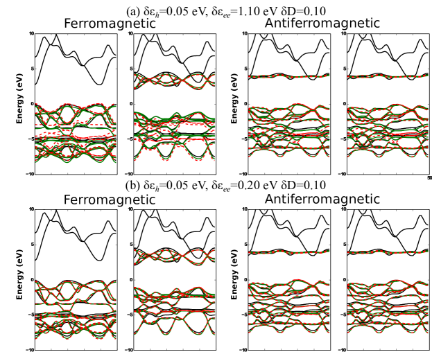
Figure 9: (Color online) Band structure of NiO as obtained for two different sets of cutoff parameters. Solid black lines represent first-principles bands obtained from LDA+U calculations, while solid green lines show the bands as obtained after filtering of $h_{\bm{a}\bm{b}}^{s}$ with a cutoff of $\delta\varepsilon_{h}$=0.05 eV [see Sec. III]. Dashed red lines represent the bands as obtained after a second filtering with (a) $\delta\varepsilon_{ee}$=1.10 eV, $\delta D$=0.10 and (b) $\delta\varepsilon_{ee}$=0.20 eV, $\delta D$=0.10

It is interesting to note that our TS does not contain enough information to fit reliably all the Ni($e_{g}$)-Ni($e_{g}$) interactions compatible with our filters. More precisely, we find that there are only two relevant $I_{\bm{a}\bm{b},\bm{a}^{\prime}\bm{b}^{\prime}}$ constants: one related to the self-energy of the $e_{g}$ states ($I_{\bm{a}\bm{a},\bm{a}\bm{a}}$, where $\bm{a}$ is a $e_{g}$-like basis function), and a second one quantifying the interaction between the two $e_{g}$ states in the same atom (essentially, the exchange interaction known as Hund’s coupling). It is clear that our TS is not suitable to distinguish between such interactions. In both the FM and AF2 phases, the Ni²⁺ ions display a $S=1$ spin configuration; yet, the interplay between self-interaction and Hund coupling only appears when trying to differentiate between the high- ($S=1$) and low- ($S=0$) spin intra-atomic states.

We checked whether such an indeterminacy affects the energy difference between the FM and AF2 phases as obtained from the model. To do so, we first add a Hubbard-U constant associated to the self-energy of the $e_{g}$ WFs, and make it equal to the corresponding $I$ constant (i.e., we impose $I_{\bm{aa}\bm{aa}}=U_{\bm{aa}\bm{aa}}$). In this way the self-interaction of an electron placed in one of these orbitals is $U-I$ = 0, while the interaction between two electrons that only differ in their spin is $U+I=2I=2U$. Then, we vary this self-interaction parameter between 0 eV and 6 eV, optimize the interaction between different $e_{g}$ orbitals to reproduce the bands, and calculate the FM–AF2 energy gap. We observe that the energy difference is quite insensitive to the value of $I_{\bm{aa}\bm{aa}}$, varying by less than 5% in the explored range. Hence, we simply take $I_{\bm{aa}\bm{aa}}$ = 2 eV to fix the indeterminacy in the model.

V.2.2 Results

Magnetism in rocksalt structures is usually described using a Heisenberg Hamiltonian with coupling constants between first- ($J_{1}$) and second- ($J_{2}$) nearest neighbors.Chatterji et al. (2009); Hutchings and Samuelsen (1972); Archer et al. (2011) These constants can be obtained from the energy differences between different spin arrangements by solving the equation system:

$$E_{\text{FM}}= E_{\text{ref}}-6J_{1} -3J_{2}$$

$$E_{\text{AF1}}= E_{\text{ref}}+2J_{1} -3J_{2}$$ (95)

$$E_{\text{AF2}}= E_{\text{ref}} +3J_{2},$$

which involves the spin arrangements of Fig. 8. $E_{\text{ref}}$ stands for the energy of a reference phase.

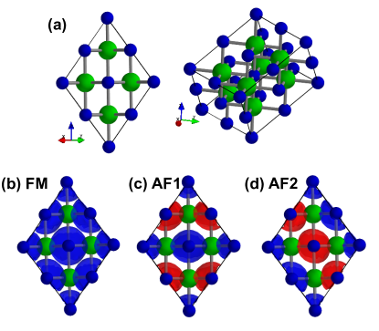
Figure 10: (Color online) Results for the $D^{I}$ difference occupation matrix in real space. In panel (a) we display the 16-ion supercell employed in the calculation along one of its main directions (left) and a general panoramic of the same cell (right). Panels (b), (c) and (d) show the $D^{I}$ distribution in real space for the FM (b), AF1 (c), and AF2 (d) phases, respectively. Blue and red regions correspond to spin-up and spin-down magnetization, respectively.

We employ our models to compute the energy of these phases, using a 2$\times$2$\times$2 supercell containing 16 atoms, as sketched in Fig. 10. After converging the calculations, we plot the spatial distribution of $D^{I}$ (using the spatial representation of the WFs in our basis) to check that the obtained solutions correctly correspond to the FM, AF1, and AF2 spin arrangements. These plots are shown in Fig. 10, where it can be seen that the electron distribution in the simulations perfectly matches the spin orderings sketched in Fig. 8. We can now check the numerical results for the phase energies obtained with the three second-principles parameterizations [denoted, respectively, SP-LDAU-Ni($e_{g}$), SP-LDAU-Ni(3$d$), and SP-LDAU-Ni+O in Table 2] and compare them to our full DFT+U result and data in the literature (see e.g. Ref. Archer et al., 2011).

Table 2: Magnetic coupling constants of NiO obtained from various experiments, first-principles, and second-principles calculations. The latter have been modeled after the LDA+U calculations and, as can be seen, converge towards the results obtained with this method when reducing $\delta\varepsilon_{ee}$.

Method	$J_{1}$ (meV)	$J_{2}$ (meV)
neutronHutchings and Samuelsen (1972)	1.4	-19.0
neutronShanker and Singh (1973)	-1.4	-17.3
HSEArcher et al. (2011)	2.3	-21.0
PSICArcher et al. (2011)	3.3	-24.7
ASICArcher et al. (2011)	5.2	-45.0
GGA+UKotani and van Shilfgaarde (2008)	1.7	-19.1
LDA+U	2.6	-17.5
SP-LDAU-Ni($e_{g}$)	-0.2	-19.1
SP-LDAU-Ni(3$d$)	-0.0	-19.1
SP-LDAU-Ni+O	3.3	-17.6

We find that the coupling constants computed from our models compare quite well with the first-principles results. Indeed, we find the $J_{2}$, running along the 180^∘ Ni–O–Ni bridge, to be much stronger than the $J_{1}$ coupling along the 90^∘ Ni–O–Ni path. It is worth noting that a parametrization as simple as that of the SP-LDAU-Ni($e_{g}$) model captures this essential feature already. Then, when we include $I$ couplings between Ni($e_{g}$) and Ni($t_{2g}$) WFs, we obtain a very similar result, with a very small $J_{1}=-0.04$ meV. Finally, when we include electron-electron couplings with the oxygen orbitals, we get a value for $J_{1}$ that is very close to the first-principles result.

V.3 Electron gas at the LaAlO₃/SrTiO₃ interface

Now we tackle the well-studied electron gas appearing at the interface between LaAlO₃ (LAO) and SrTiO₃ (STO). The origin of the 2DEG has been intensively debated in the literature.Hwang et al. (2012); Bristowe et al. (2014) Here we are going to consider an idealized defect-free interface in which the driving force for the 2DEG is the so-called polar catastrophe that was proposed originally,Ohtomo and Hwang (2004); Nakagawa et al. (2006) which arises from the charge discontinuity between LaAlO₃ and SrTiO₃ when the bilayer is grown along the (001) pseudo-cubic direction of the perovskite lattice.Stengel and Vanderbilt (2009) In such a case, the occurrence of the metallic state strongly depends on the electrostatic boundary conditions on each side of the interface.Stengel (2011) Let us look at them in some detail to establish the basic elements of the calculation.

From simple electrostatic arguments we know that

$$D_{\text{LAO}}-D_{\text{STO}}=\sigma_{\text{free}},$$ (96)

where $D_{\text{LAO}}$ and $D_{\text{STO}}$ are the normal components of the displacement field in LaAlO₃ and SrTiO₃, respectively, and $\sigma_{\text{free}}$ is the free charge density at the interface between the materials. Hence, depending on the particular values of $D_{\text{LAO}}$ and $D_{\text{STO}}$ (which can be controlled in a simulation by varying the charges at the open surfaces of the layersStengel (2011)), a 2DEG appears at the interface according to Eq. (96). Figure 11(b) illustrates the case for a partial compensation ($D_{\text{STO}}=0$, and $D_{\text{LAO}}<-0.5$, both in units of electrons per surface unit cell), which correspond to the case of a partial transfer of charge from the LaAlO₃ surface to the interface due to the crossing of the top of the valence band of LaAlO₃ with the bottom of the conduction band of SrTiO₃. (The interface free carriers occupy states in the conduction band of SrTiO₃.) When there is no full compensation an electric field is present in the LaAlO₃ layer.

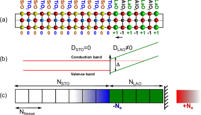
Figure 11: (Color online) Schematic representation of a polar (001) SrTiO₃/LaAlO₃ interface. Atoms are represented by balls: O (red), Ti (blue), Sr (yellow), Al (black), and La (green). A free LaO-terminated surface of LaAlO₃ is assumed. Numbers below each layer indicate formal ionic charge. The built-in polarization of SrTiO₃ (null) and LaAlO₃ is illustrated by black arrows. (b) Schematic representation of the energy bands in the case of partial compensation of the polar discontinuity at the interface. $\Delta$ represents the LaAlO₃ gap. (c) Set-up of the second-principles simulation for this interface. White and dark green squares represent, respectively, SrTiO₃ and LaAlO₃ cells. The metallic states in SrTiO₃, containing $N_{e}$ electrons per cell, are represented here by a blue gradient. To be consistent with the electrostatic boundary conditions we use the charge image method, represented here by a positive charge distribution (red gradient) on the LaAlO₃ side. The meaning of $N_{\text{STO}}$, $N_{\text{LAO}}$ and $N_{\text{freeze}}$ is explained in the text.

This setup is ideal to test our method, since the main physical effects are related to the negative doping of SrTiO₃, such a doping being controlled by the electrostatic boundary conditions. Further, the properties of the 2DEG (e.g., spatial extension) depend essentially on the ability of SrTiO₃ to screen these additional charges, which in turn involves the electron-lattice couplings in our models.

We simulate the LaAlO₃/SrTiO₃ interface [Fig. 11(c)] by considering a slab of $N=N_{\text{LAO}}+N_{\text{STO}}$ 5-atom perovskite unit cells, where the first $N_{\text{LAO}}$ cells are occupied by LaAlO₃ and the following $N_{\text{STO}}$ cells by SrTiO₃. Following Stengel,Stengel (2011) we do not consider the electronic details of the interface, as these were found to be of little relevance to describe the main physical features of the 2DEG. In fact, as regards the construction of our model, we treat the entire slab as if it was made of SrTiO₃, but introducing the following modifications: (i) on the LaAlO₃ side, the levels of the conduction band are shifted up (by appropriately modifying the $\gamma_{\bm{a}\bm{a}}$ self-energies) so that they do not interact with those on the SrTiO₃ side, and (ii) to account for the large disparity between the LaAlO₃ and SrTiO₃ dielectric constants (the latter is around 25 times larger than the former at room temperature) we simply freeze the coordinates of the atoms on the LaAlO₃ layer at the RAG, to prevent atomic displacements from screening electric fields.

As regards the electrostatic boundary conditions, we consider that $D_{\text{STO}}=0$ and $D_{\text{LAO}}=-N_{e}/S$, i.e., we have $N_{e}$ electrons per unit area $S$ doping the slab. To impose such conditions, we first freeze into the centrosymmetric structure the atomic positions of $N_{\text{freeze}}$ unit cells at the end of the SrTiO₃ side of the slab [see Fig. 11(c)]. Secondly, we use the image-charge methodJackson (1975) [see Fig. (11)c] to introduce an electric field from the LaAlO₃ side of the interface consistent with $D_{\text{LAO}}=-N_{e}/S$.

V.3.1 Model parameters

We now describe how we obtain the parameters for the SrTiO₃ layer. As already mentioned, SrTiO₃ is a non-magnetic insulator and the RED corresponds to the ground state of the undoped system. This allows us to take the lattice potential for pure SrTiO₃ described in Ref. Wojdeł et al., 2013 as the $E^{(0)}$ term of our model [see Eqs. (5) and  (6)], using the LDA-relaxed cubic phase as RAG. [We slightly modified the force field of Ref. Wojdeł et al., 2013, by tuning the interaction between first-nearest-neighbouring Ti and O pairs, to exactly reproduce a dielectric constant of 500 for the cubic phase (see Fig. 12), as obtained from LDA calculations in Ref. Stengel, 2011].

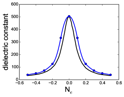
Figure 12: (Color online) Dielectric constant of SrTiO₃ as calculated in LDA Stengel (2011) (solid black line) and with our second-principles method (solid blue circles and line) as a function of the electric displacement field, i.e., as a function of the number of electrons per surface unit doping the interface.

We then extended the model to include the electronic states associated with the bottom of the conduction band of SrTiO₃, which present a dominant Ti($t_{2g}$) character [see Fig. 3(a)]. We followed the recipe in Sec. III to extract the $\gamma$ parameters describing these bands.

Note that our focus in this application was to capture the electron-lattice effects that determine the properties of the 2DEG, and we were not concerned with electron-electron couplings beyond the LDA. Thus, we did not include $U$ or $I$ terms in our model, and used a TS that contains the RAG and distorted structures (with individual atoms displaced by 0.05 Å, 0.10 Å, and 0.15 Å from their RAG positions), all of which where assumed to be in the RED state.

We then found all $\gamma$, $\vec{\bm{f}}$ and $\overleftrightarrow{\bm{g}}$ parameters [Eq. (62)] compatible with the choices $\delta\varepsilon_{h}$ = 0.05 eV and $\delta f_{e-l}$ = 1.0 eV/Å. We observe that the electron-lattice constants associated to diagonal one-electron terms, $\gamma_{\bm{a}\bm{a}}$, are much more sensitive to the displacement of the ions than the off-diagonal ones. The distortions that induce larger changes involve the Ti–O bond, as expected according to the long literature on covalency in ferroelectric oxides and related materials.Bersuker (2006); Cohen (1992); Cohen and Krakauer (1990); Posternak et al. (1994)

Finally, we took the Born charges and high-frequency dielectric tensor used in our lattice model, $E^{(0)}$, to compute the electrostatic energy associated to the electronic degrees of freedom.

V.3.2 Results

We now compare the results for the LaAlO₃/SrTiO₃ interface obtained with the above-described model and the LDA results of Ref. Stengel, 2011, where the calculations were performed for $N_{\text{LAO}}$ = 5 and $N_{\text{STO}}$ = 12. Using these values, we carry out geometry optimizations with the constraints illustrated in Fig. 11(c). The results of these calculations are shown in Figs. 13(a) and 13(b), where we compare the electron densities from first-principles LDA and second-principles simulations for $N_{e}$ = 0.3 and $N_{e}$ = 0.5, respectively. Moreover, in Figs. 13(c) and 13(d) we show the obtained lattice distortions, in terms of the layer-by-layer rumpling, for the same cases.

We can observe that the second-principles and LDA results match well for both atomic and electronic structure. Moreover, following the discussion in Ref. Stengel, 2011, we checked that our model captures correctly the influence that various physical parameters (e.g., linear and non-linear response of the lattice, etc.) have in the final result. As regards relatively small errors in the shape of the electronic density profiles, we attribute them to technical differences (pseudopotentials, etc.) in the LDA calculations of Ref. Stengel, 2011 and those performed to construct our models.

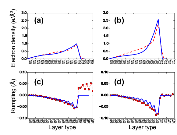
Figure 13: (Color online) Results for the 2DEG at the LaAlO₃/SrTiO₃ interface. The second-principles results are indicated with solid blue lines, while the LDA results are given by dashed red lines. Panels (a) and (b) show the electron density distribution for $N_{e}$=0.3, and $N_{e}$=0.5, respectively. Panels (c) and (d) show the rumpling of the lattice for the same two cases.

V.4 Additional considerations

To finish this section we would like to give some estimations of the computer time required to carry out the second-principles calculations for the systems discussed in the present work. We will focus first on NiO, as we carried out both the DFT and second-principles computations for the same unit cells and on the same computational platform, so a reliable comparison of timings should be feasible. In Table 3 we show the time necessary to perform a single-point calculation using a single CPU, using the same reciprocal space sampling in the LDA+U and second-principles simulations. The values for 4- and 16-ion cells clearly show the very large speed-up of our second-principles simulations when compared to standard DFT even in small cells. Looking at Table 3 we see that there are very small differences between the timing results between the different parameterizations associated to different levels of description of the electron-electron interactions in NiO. Finally, in order to give an estimation of the scaling of the method as it stands now (i.e., at an early stage of implementation), we carried out a calculation of a 10$\times$10$\times$10 periodic supercell that contains 2000 atoms. This is approximately the size limit for single-point DFT calculations, and it would require significant computational resources and a highly parallelized code. However, this simulation at the SP-LDAU-Ni($e_{g}$) level took 6.6 hours of a single CPU, suggesting that calculations including tens of thousands of atoms are within reach using our models.

Table 3: Simulation running times on a single CPU for the 4-ion 1$\times$1$\times$2, 16-ion 2$\times$2$\times$2 and 2000-ion 10$\times$10$\times$10 NiO supercells. The lower time obtained for the SP-LDAU-Ni(3$d$) with respect to SP-LDAU-Ni($e_{g}$) is due to the smaller number of self-consistent steps required in the former simulation.

Method	4 ion (s)	16 ion (s)	2000 ion (hours)
LDA+U	65.0	3516.8	—
SP-LDAU-Ni($e_{g}$)	1.4	14.5	6.63
SP-LDAU-Ni(3$d$)	1.4	14.1	6.59
SP-LDAU-Ni+O	1.5	15.8	6.97

Turning now to the simulation of the LaAlO₃/SrTiO₃ interface we note that each of the geometry optimizations involving a 85-atom supercell took about 13 minutes using a single desktop CPU.

VI Concluding remarks

In this work we have presented a first-principles-based multi-scale method, which we denominate second-principles, that makes it possible to compute the properties of materials at an atomic level, with an accuracy essentially equal to DFT, and at a very reduced computational cost.

Our approach is based on dividing the electron density of the system into a reference part, usually corresponding to its neutral ground state at any geometry, and a deformation part, defined as the difference between the actual and reference densities. We take advantage of the fact that the largest part of the system’s energy depends on the reference density, and can be efficiently and accurately described by a force field with no explicit consideration of the electrons. Then, the effects associated to the difference density can be treated perturbatively with good precision by working in the Wannier function basis corresponding to the reference state. Further, the electronic description can be restricted to the bands of interest, which renders a computationally very efficient scheme.

Conceptually, the present approach constitutes a fresh look at the problem of how to describe lattice and electronic degrees of freedom simultaneously and effectively, introducing a convenient partition of the energy that permits an accurate treatment of both types of variables and their mutual interactions. In our view, our method constitutes a significant step beyond the usual techniques – ranging from molecular-mechanics to tight-binding and quantum-mechanics/molecular-mechanics schemes – towards a more unified model.

As illustrated by the examples described here, the present approach allows us to obtain DFT-like accuracy in the analysis of subtle physical effects, like those determining the relative stability of the magnetic phases of NiO, or those involved in the structural relaxations and screening processes associated to the two-dimensional electron gas formed at the interface of LaAlO₃ and SrTiO₃. Note that these problems – which involve electron correlation effects, transition-metal ions, etc. – are usually hard to treat within DFTB schemes.Zheng et al. (2007)

As currently formulated, our approach has only one essential limitation: it is restricted to systems in which it is possible to (loosely) define an underlying bonding topology that is to be preserved. Hence, while the method allows the system undergo significant structural modifications – e.g., like those involved in typical ferroelectric or ferroelastic phase transitions –, it is not possible to study full-blown bond breaking directly with it. Nevertheless, this limitation can be overcome by using our method in multi-scale simulations that permit a more detailed treatment (e.g., with DFT) of the regions of the material in which the constant-topology condition is not satisfied.

It is also important to note that the constant-topology condition is perfectly compatible with the study of many structurally non-trivial cases, such as nanostructured materials, surfaces, chemically-disordered solid solutions, coexistence of different structural and electronic phases, etc. Hence, the application scope of our scheme is enormous.

Let us also note that the present method can be extended to cover physical effects not mentioned here. For example, it is possible to expand it to treat relativistic phenomena (as spin-orbit effects) or time-dependent non-equilibrium situations (as resulting from the interaction with light) in essentially the same way as the initial DFT implementations were extended to do so (by implementing a non-colinear treatment of magnetism, time-dependent DFT, etc.). Further, since our method provides us with a Hamiltonian for the interacting system, one could imagine solving the electronic problem in ways that go beyond the mean-field approach adopted here, and thus better account for many body effects.

The ability to simulate systems with thousands of atoms, treating both lattice and electrons accurately, may permit for the first time predictive investigations of a variety of intriguing phenomena – e.g., Mott transitions, coupled spin-lattice dynamics, charged and conducting domain walls, polaron transport, etc. – in realistic conditions of temperature, applied fields, etc. We thus believe that the present method has the potential to significantly advance our understanding of some of today’s most interesting problems in condensed-matter physics and material science.

Appendix A Expanding the total energy with respect to the deformation density

The total electronic density of the system can be written as the sum of a reference electronic density, $n_{0}(\vec{r})$, and a small deformation electron density, $\delta n(\vec{r})$, defined as in Eq. (2). Inserting this into the expression for the total DFT energy, Eq. (3), and considering also the expansion of the exchange and correlation energy upto second order in the deformation energy, Eq. (4), then

$$E_{\text{DFT}}\approx \sum_{j\vec{k}}o_{j\vec{k}}\left\langle\psi_{j\vec{k}}\right|\hat{t}+v_{\text{ext}}\left|\psi_{j\vec{k}}\right\rangle+$$

$$+\frac{1}{2}\iint\frac{n_{0}(\vec{r})n_{0}(\vec{r}\mkern 2.0mu\vphantom{r}^{\prime})}{|\vec{r}-\vec{r}\mkern 2.0mu\vphantom{r}^{\prime}|}d^{3}rd^{3}r^{\prime}$$

$$+\frac{1}{2}\iint\frac{\delta n(\vec{r})\delta n(\vec{r}\mkern 2.0mu\vphantom{r}^{\prime})}{|\vec{r}-\vec{r}\mkern 2.0mu\vphantom{r}^{\prime}|}d^{3}rd^{3}r^{\prime}$$

$$+\iint\frac{n_{0}(\vec{r}\mkern 2.0mu\vphantom{r}^{\prime})\delta n(\vec{r})}{|\vec{r}-\vec{r}\mkern 2.0mu\vphantom{r}^{\prime}|}d^{3}rd^{3}r^{\prime}+E_{\text{xc}}[n_{0}]$$

$$+\int\left.\frac{\delta E_{\text{xc}}}{\delta n(\vec{r})}\right|_{n_{0}}\delta n(\vec{r})d^{3}r$$

$$+\frac{1}{2}\iint\left.\frac{\delta^{2}E_{\text{xc}}}{\delta n(\vec{r})\delta n(\vec{r}\mkern 2.0mu\vphantom{r}^{\prime})}\right|_{n_{0}}\delta n(\vec{r})\delta n(\vec{r}\mkern 2.0mu\vphantom{r}^{\prime})d^{3}rd^{3}r^{\prime}$$

$$+E_{\text{nn}}.$$ (97)

Adding and substracting $\sum_{j\vec{k}}o^{(0)}_{j\vec{k}}\langle\psi^{(0)}_{j\vec{k}}|\hat{t}+v_{\text{ext}}|\psi^{(0)}_{j\vec{k}}\rangle$, where $|\psi^{(0)}_{j\vec{k}}\rangle$ and $o^{(0)}_{j\vec{k}}$ are the eigenvectors and the occupation numbers for the $j$-band of the wavevector $\vec{k}$ that define the reference electron density for a given atomic configuration, and grouping together the terms at zero, first and second order in the deformation electronic density, we can write

$$E_{\text{DFT}}\approx E^{(0)}+E^{(1)}+E^{(2)}.$$ (98)

The zero order term $E^{(0)}$, amounts to

$$E^{(0)}= \sum_{j\vec{k}}o^{(0)}_{j\vec{k}}\left\langle\psi^{(0)}_{j\vec{k}}\right|\hat{t}+v_{\text{ext}}\left|\psi^{(0)}_{j\vec{k}}\right\rangle$$

$$+\frac{1}{2}\iint\frac{n_{0}(\vec{r})n_{0}(\vec{r}\mkern 2.0mu\vphantom{r}^{\prime})}{|\vec{r}-\vec{r}\mkern 2.0mu\vphantom{r}^{\prime}|}d^{3}rd^{3}r^{\prime}$$

$$+E_{\text{xc}}[n_{0}]+E_{\text{nn}}.$$ (99)

The first order term $E^{(1)}$ takes the following expression

$$E^{(1)}= \sum_{j\vec{k}}o_{j\vec{k}}\left\langle\psi_{j\vec{k}}\right|\hat{t}+v_{\text{ext}}\left|\psi_{j\vec{k}}\right\rangle-\sum_{j\vec{k}}o^{(0)}_{j\vec{k}}\left\langle\psi^{(0)}_{j\vec{k}}\right|\hat{t}+v_{\text{ext}}\left|\psi^{(0)}_{j\vec{k}}\right\rangle+\iint\frac{n_{0}(\vec{r}\mkern 2.0mu\vphantom{r}^{\prime})\delta n(\vec{r})}{|\vec{r}-\vec{r}\mkern 2.0mu\vphantom{r}^{\prime}|}d^{3}rd^{3}r^{\prime}+\int\left.\frac{\delta E_{\text{xc}}}{\delta n(\vec{r})}\right|_{n_{0}}\delta n(\vec{r})d^{3}r$$

$$= \sum_{j\vec{k}}o_{j\vec{k}}\left\langle\psi_{j\vec{k}}\right|\hat{t}+v_{\text{ext}}\left|\psi_{j\vec{k}}\right\rangle-\sum_{j\vec{k}}o^{(0)}_{j\vec{k}}\left\langle\psi^{(0)}_{j\vec{k}}\right|\hat{t}+v_{\text{ext}}\left|\psi^{(0)}_{j\vec{k}}\right\rangle-\int v_{\text{H}}(n_{0};\vec{r})\delta n(\vec{r})d^{3}r+\int v_{\text{xc}}[n_{0};\vec{r}]\delta n(\vec{r})d^{3}r$$

$$= \sum_{j\vec{k}}o_{j\vec{k}}\left\langle\psi_{j\vec{k}}\right|\hat{t}+v_{\text{ext}}\left|\psi_{j\vec{k}}\right\rangle-\sum_{j\vec{k}}o^{(0)}_{j\vec{k}}\left\langle\psi^{(0)}_{j\vec{k}}\right|\hat{t}+v_{\text{ext}}\left|\psi^{(0)}_{j\vec{k}}\right\rangle+\int\left[-v_{\text{H}}(n_{0};\vec{r})+v_{\text{xc}}[n_{0};\vec{r}]\right]\left(n(\vec{r})-n_{0}(\vec{r})\right)d^{3}r$$

$$= \sum_{j\vec{k}}o_{j\vec{k}}\left\langle\psi_{j\vec{k}}\right|\hat{t}+v_{\text{ext}}\left|\psi_{j\vec{k}}\right\rangle-\sum_{j\vec{k}}o^{(0)}_{j\vec{k}}\left\langle\psi^{(0)}_{j\vec{k}}\right|\hat{t}+v_{\text{ext}}\left|\psi^{(0)}_{j\vec{k}}\right\rangle$$

$$+\sum_{j\vec{k}}\int o_{j\vec{k}}\left\langle\psi_{j\vec{k}}\right|-v_{\text{H}}(n_{0};\vec{r})+v_{\text{xc}}[n_{0};\vec{r}]\left|\psi_{j\vec{k}}\right\rangle d^{3}r-\sum_{j\vec{k}}\int o^{(0)}_{j\vec{k}}\left\langle\psi^{(0)}_{j\vec{k}}\right|-v_{\text{H}}(n_{0};\vec{r})+v_{\text{xc}}[n_{0};\vec{r}]\left|\psi^{(0)}_{j\vec{k}}\right\rangle d^{3}r$$

$$= \sum_{j\vec{k}}o_{j\vec{k}}\left\langle\psi_{j\vec{k}}\right|\hat{t}+v_{\text{ext}}-v_{\text{H}}(n_{0};\vec{r})+v_{\text{xc}}[n_{0};\vec{r}]\left|\psi_{j\vec{k}}\right\rangle-\sum_{j\vec{k}}\int o^{(0)}_{j\vec{k}}\left\langle\psi^{(0)}_{j\vec{k}}\right|\hat{t}+v_{\text{ext}}-v_{\text{H}}(n_{0};\vec{r})+v_{\text{xc}}[n_{0};\vec{r}]\left|\psi^{(0)}_{j\vec{k}}\right\rangle$$

$$= \sum_{j\vec{k}}o_{j\vec{k}}\left\langle\psi_{j\vec{k}}\right|\hat{h}_{0}\left|\psi_{j\vec{k}}\right\rangle-\sum_{j\vec{k}}\int o^{(0)}_{j\vec{k}}\left\langle\psi^{(0)}_{j\vec{k}}\right|\hat{h}_{0}\left|\psi^{(0)}_{j\vec{k}}\right\rangle,$$ (100)

where we have defined the Kohn-Sham one electron hamiltonian defined for the reference state density $n_{0}$ as

$$\hat{h}_{0}=\hat{t}+v_{\text{ext}}-v_{\text{H}}(n_{0};\vec{r})+v_{\text{xc}}[n_{0};\vec{r}],$$ (101)

with the reference Hartree potential

$$v_{\text{H}}(n_{0};\vec{r})=-\int\frac{n_{0}(\vec{r}\mkern 2.0mu\vphantom{r}^{\prime})}{|\vec{r}-\vec{r}\mkern 2.0mu\vphantom{r}^{\prime}|}d^{3}r^{\prime},$$ (102)

and the exchange and correlation potential

$$v_{\text{xc}}[n_{0};\vec{r}]=\left.\frac{\delta E_{\text{xc}}[n]}{\delta n(\vec{r})}\right|_{n_{0}}.$$ (103)

The second order term $E^{(2)}$ can be written as

$$E^{(2)}= \frac{1}{2}\iint\frac{\delta n(\vec{r})\delta n(\vec{r}\mkern 2.0mu\vphantom{r}^{\prime})}{|\vec{r}-\vec{r}\mkern 2.0mu\vphantom{r}^{\prime}|}d^{3}rd^{3}r^{\prime}$$

$$+\frac{1}{2}\iint\left.\frac{\delta^{2}E_{\text{xc}}}{\delta n(\vec{r})\delta n(\vec{r}\mkern 2.0mu\vphantom{r}^{\prime})}\right|_{n_{0}}\delta n(\vec{r})\delta n(\vec{r}\mkern 2.0mu\vphantom{r}^{\prime})d^{3}rd^{3}r^{\prime}$$ (104)

Appendix B Inverse transformation from the Wannier to Bloch functions

We start from the definition of the Wannier functions from an isolated manifold of $J$ Bloch orbitals, Eq. (13),

$$|\chi_{\bm{a}}\rangle\equiv|\vec{R}_{A}a\rangle=\frac{V}{2\pi^{3}}\int_{\rm BZ}d\vec{k}\>\>e^{-i\vec{k}\cdot\vec{R}_{A}}\sum_{m=1}^{J}T_{ma}^{(\vec{k})}|\psi_{m\vec{k}}^{(0)}\rangle,$$ (105)

where the $\bm{T}^{(\vec{k})}$ matrices are the unitary transformations that minimize the localization functional. The Bloch orbitals are those that define the reference density for a given atomic geometry, i.e., those used to construct the Wannier functions.

Then, multiplying both sides of the equation by $e^{i\vec{k}^{\prime}\cdot\vec{R}_{A}}$ and summing over all the lattice sites in real space

$$\sum_{\vec{R}_{A}}e^{i\vec{k}^{\prime}\cdot\vec{R}_{A}}|\vec{R}_{A}a\rangle=$$

$$=\frac{V}{(2\pi)^{3}}\int_{\rm BZ}d\vec{k}\>\>\left[\sum_{\vec{R}_{A}}e^{i\left(\vec{k}^{\prime}-\vec{k}\right)\cdot\vec{R}_{A}}\right]\sum_{m=1}^{J}T_{ma}^{(\vec{k})}|\psi_{m\vec{k}}^{(0)}\rangle$$

$$=\int_{\rm BZ}d\vec{k}\>\>\delta(\vec{k}^{\prime}-\vec{k})\sum_{m=1}^{J}T_{ma}^{(\vec{k})}|\psi_{m\vec{k}}^{(0)}\rangle$$

$$=\sum_{m=1}^{J}|\psi_{m\vec{k}^{\prime}}^{(0)}\rangle T_{ma}^{(\vec{k}^{\prime})}.$$ (106)

Finally, multiplying both sides of Eq. (106) by the inverse matrix of the unitary transformation

$$\sum_{a=1}^{J}\sum_{\vec{R}_{A}}e^{i\vec{k}^{\prime}\cdot\vec{R}_{A}}|\vec{R}_{A}a\rangle\left(T_{al}^{(\vec{k}^{\prime})}\right)^{-1}=$$

$$=\sum_{m=1}^{J}|\psi_{m\vec{k}^{\prime}}^{(0)}\rangle\sum_{a=1}^{J}T_{ma}^{(\vec{k}^{\prime})}\left(T_{al}^{(\vec{k}^{\prime})}\right)^{-1}$$

$$=\sum_{m=1}^{J}|\psi_{m\vec{k}^{\prime}}^{(0)}\rangle\delta_{ml}$$

$$=|\psi_{l\vec{k}^{\prime}}^{(0)}\rangle.$$ (107)

This expression can be rewritten as

$$|\psi_{l\vec{k}}^{(0)}\rangle =\sum_{\bm{a}}\left(T_{al}^{(\vec{k})}\right)^{-1}e^{i\vec{k}\cdot\vec{R}_{A}}|\vec{R}_{A}a\rangle\noindent$$ (108)

$$=\sum_{{\bm{a}}}c_{la\vec{k}}^{(0)}\>\>e^{i\vec{k}\cdot\vec{R}_{A}}|\vec{R}_{A}a\rangle,$$ (109)

that is the same as Eq. (14) with the role of the coefficients of the expansion played by the elements of the inverse matrix of the unitary transformation.

References

- Kohn and Sham (1965) W. Kohn and L. J. Sham, Phys. Rev. 140, A1133 (1965).
- Parr and Yang (1994) R. Parr and W. Yang, Density-Functional Theory of Atoms and Molecules (Oxford University Press, New York, 1994).
- Martin (2004) R. M. Martin, Electronic Structure. Basic Theory and Practical Methods (Cambridge University Press, Cambridge, 2004).
- Jensen (1999) F. Jensen, Introduction to Computational Chemistry (John Wiley & Sons, Chichester, England, 1999).
- Kohanoff (2006) J. Kohanoff, Electronic structure calculations for solids and molecules (Cambridge University Press, Cambridge, 2006).
- Slater and Koster (1954) J. C. Slater and G. F. Koster, Phys. Rev. 94, 1498 (1954).
- Harrison (1988) W. A. Harrison, Electronic Structure and the Propeties of Solids (Dover, Mineola, New York, 1988).
- Lifson and Warshel (1968) S. Lifson and A. Warshel, J. Chem. Phys. 49, 5116 (1968).
- Brown (2009) I. D. Brown, Chem. Rev. 109, 6858 (2009).
- Porezag et al. (1995) D. Porezag, T. Fruenheim, T. Köhler, G. Seifert, and R. Kaschner, Phys. Rev. B 51, 12947 (1995).
- Matthew et al. (1989) W. Matthew, C. Foulkes, and R. Haydock, Phys. Rev. B 39, 12520 (1989).
- Elstner et al. (1998) M. Elstner, D. Porezag, G. Jungnickel, J. Elsner, M. Haugk, T. Frauenheim, S. Suhai, and G. Seifert, Phys. Rev. B 58, 7260 (1998).
- Harris (1998) J. Harris, Phys. Rev. B 31, 1770 (1998).
- Sankey and Niklewski (1989) O. F. Sankey and D. J. Niklewski, Phys. Rev. B 40, 3979 (1989).
- Lewis et al. (2011) J. P. Lewis, P. Jelínek, J. Ortega, A. A. Demkov, D. G. Trabada, B. Haycock, H. Wang, G. Adams, J. K. Tomfohr, E. Abad, H. Wang, and D. A. Drabold, Phys. Status Solidi B 211, 1989 (2011).
- Joannopoulos and Rabe (1987) J. A. Joannopoulos and K. M. Rabe, Phys. Rev. Lett. 59, 570 (1987).
- Zhong et al. (1994) W. Zhong, D. Vanderbilt, and K. M. Rabe, Phys. Rev. Lett. 73, 1861 (1994).
- Zhong et al. (1995) W. Zhong, D. Vanderbilt, and K. M. Rabe, Phys. Rev. B 52, 6301 (1995).
- Bellaiche et al. (2000) L. Bellaiche, A. García, and D. Vanderbilt, Phys. Rev. Lett. 84, 5427 (2000).
- Rahmedov et al. (2012) D. Rahmedov, D. Wang, J. Íñiguez, and L. Bellaiche, Phys. Rev. Lett. 109, 037207 (2012).
- Gaus et al. (2011) M. Gaus, Q. Cui, and M. Elstner, J. Chem. Theory Comput. 7, 931 (2011).
- Riccardi et al. (2006) D. Riccardi, P. Schaefer, Y. Yang, H. Yu, N. Ghosh, X. Prat-Resina, P. K. nig, G. Li, D. Xu, H. Guo, M. Elstner, and Q. Cui, J. Phys. Chem. B 110, 6458 (2006).
- Giese and York (2012) T. J. Giese and D. M. York, Theor. Chem. Acc. 131, 1145 (2012).
- Hubbard (1963) J. Hubbard, Proc. Roy. Soc. (London) A276, 238 (1963).
- Spałek (1988) J. Spałek, Phys. Rev. B 37, 533 (1988).
- Kugel and Khomskii (1973) K. J. Kugel and D. I. Khomskii, Sov. Phys. - JETP 37, 725 (1973).
- Millis et al. (1996) A. J. Millis, B. I. Shralman, and R. Mueller, Phys. Rev. Lett. 77, 175 (1996).
- Stengel (2011) M. Stengel, Phys. Rev. Lett. 106, 136803 (2011).
- Kornev et al. (2007) I. A. Kornev, S. Lisenkov, R. Haumont, B. Dkhil, and L. Bellaiche, Phys. Rev. Lett. 99, 227602 (2007).
- Wojdeł et al. (2013) J. C. Wojdeł, P. Hermet, M. P. Ljungberg, P. Ghosez, and J. Íñiguez, J. Phys.: Cond. Matter 25, 305401 (2013).
- Soler et al. (2002) J. M. Soler, E. Artacho, J. D. Gale, A. García, J. Junquera, P. Ordejón, and D. Sánchez-Portal, J. Phys.: Condens. Matter 14, 2745 (2002).
- Payne et al. (1992) M. Payne, M. Teter, D. Allan, T. Arias, and J. Joannopoulos, Rev. Mod. Phys. 64, 1045 (1992).
- Gonze (1995) X. Gonze, Phys. Rev. A 52, 1096 (1995).
- Gonze (1997) X. Gonze, Phys. Rev. B 55, 10337 (1997).
- Parr and Pearson (1983) R. G. Parr and R. G. Pearson, J. Am. Chem. Soc. 105, 7512 (1983).
- Souza et al. (2001) I. Souza, N. Marzari, and D. Vanderbilt, Phys. Rev. B 65, 035109 (2001).
- Callaway and Hughes (1967) J. Callaway and A. J. Hughes, Phys. Rev. 156, 860 (1967).
- Teichler (1971) H. Teichler, Phys. Status Solidi B 43, 307 (1971).
- Satpathy and Pawlowska (1988) S. Satpathy and Z. Pawlowska, Phys. Status Solidi B 145, 555 (1988).
- Marzari and Vanderbilt (1997) N. Marzari and D. Vanderbilt, Phys. Rev. B 56, 12847 (1997).
- Sakura (2013) R. Sakura, Phys. Rev. B 87, 235109 (2013).
- Wang et al. (2014) R. Wang, E. A. Lazar, H. Park, A. J. Millis, and C. A. Marianetti, Phys. Rev. B 90, 165125 (2014).
- Marzari et al. (2012) N. Marzari, A. A. Mostofi, J. R. Yates, I. Souza, and D. Vanderbilt, Rev. Mod. Phys. 84, 1419 (2012).
- Marzari et al. (1997) N. Marzari, D. Vanderbilt, and M. C. Payne, Phys. Rev. Lett. 79, 1337 (1997).
- Cazorla and Íñiguez (2013) C. Cazorla and J. Íñiguez, Phys. Rev. B 88, 214430 (2013).
- Anisimov et al. (1997) V. Anisimov, F. Aryasetiawan, and A. Liechtenstein, J. Phys.: Condens. Matter 9, 767 (1997).
- Liechtenstein et al. (1995) A. Liechtenstein, V. Anisimov, and J. Zaanen, Phys. Rev. B 52, 5467 (1995).
- Hedin (1965) L. Hedin, Phys. Rev. A139, 796 (1965).
- Aryasetiawan and Gunnarsson (1998) F. Aryasetiawan and O. Gunnarsson, Rep. Prog. Phys. 61, 237 (1998).
- Stoner (1936) E. C. Stoner, Proc. R. Soc. A 154, 656 (1936).
- Gunnarson (1976) O. Gunnarson, J. Phys. F 6, 587 (1976).
- Stöhr and Siegmann (2006) J. Stöhr and H. C. Siegmann, Magnetism: From Fundamentals to Nanoscale Dynamics (Springer-Verlag, Heidelberg, 2006).
- Demkov et al. (1995) A. A. Demkov, J. Ortega, O. F. Sankey, and M. P. Grumbach, Phys. Rev. B 52, 1618 (1995).
- Jackson (1975) J. D. Jackson, Classical Electrodynamics (John Wiley & Sons, New York, 1975).
- Note (1) For metallic systems the definition and calculation of these interactions requires an adequate treatment of the screening. This problem will be addressed in future publications.
- Kugel and Khomskii (1982) K. L. Kugel and D. I. Khomskii, Sov. Phys. Usp. 25, 231 (1982).
- Bersuker (2006) I. B. Bersuker, The Jahn-Teller Effect (Cambridge University Press, Cambridge, 2006).
- Emin (2013) D. Emin, Polarons (Cambridge University Press, New York, 2013).
- García-Fernández and Bersuker (2011) P. García-Fernández and I. B. Bersuker, Phys. Rev. Lett. 106, 246406 (2011).
- García-Fernández et al. (2011) P. García-Fernández, J. A. Aramburu, and M. Moreno, Phys. Rev. B 83, 174406 (2011).
- Pulay (1969) P. Pulay, Mol. Phys. 17, 197 (1969).
- Kawata et al. (2001) M. Kawata, M. Mikami, and U. Nagashima, Chem. Phys. 115, 4457 (2001).
- Mostofi et al. (2008) A. A. Mostofi, J. R. Yates, Y.-S. Lee, I. Souza, D. Vanderbilt, and N. Marzari, Comput. Phys. Commun. 178, 685 (2008).
- Anisimov and Gunnarsson (1991) V. I. Anisimov and O. Gunnarsson, Phys. Rev. B 43, 7570 (1991).
- Solovyev (2008) I. V. Solovyev, J. Phys.: Condens. Matter. 20, 293201 (2008).
- Solovyev and Imada (2005) I. V. Solovyev and M. Imada, Phys. Rev. B 71, 045103 (2005).
- Gunnarsson et al. (1989) O. Gunnarsson, O. K. Andersen, O. Jepsen, and J. Zaanen, Phys. Rev. B 39, 1708 (1989).
- Miyake and Aryasetiawan (2008) T. Miyake and F. Aryasetiawan, Phys. Rev. B 77, 085122 (2008).
- Nakamura et al. (2006) K. Nakamura, R. Arita, Y. Yoshimoto, and S. Tsuneyuki, Phys. Rev. B 74, 235113 (2006).
- Vaugier et al. (2012) L. Vaugier, H. Jiang, and S. Biermann, Phys. Rev. B 86, 165105 (2012).
- Makov and Payne (1995) G. Makov and M. C. Payne, Phys. Rev. B 51, 4014 (1995).
- Ohtomo and Hwang (2004) A. Ohtomo and H. Y. Hwang, Nature 427, 423 (2004).
- Nakagawa et al. (2006) N. Nakagawa, H. Y. Hwang, and D. A. Muller, Nat. Mater. 5, 204 (2006).
- Bristowe et al. (2014) N. C. Bristowe, P. Ghosez, P. B. Littlewood, and E. Artacho, J. Phys.: Condens. Matter 26, 143201 (2014), (and references therein).
- Kresse and Fürthmuller (1996) G. Kresse and J. Fürthmuller, Phys. Rev. B 54, 11169 (1996).
- Kresse and Joubert (1999) G. Kresse and D. Joubert, Phys. Rev. B 59, 1758 (1999).
- Blöchl (1994) P. E. Blöchl, Phys. Rev. B 50, 17953 (1994).
- Dudarev et al. (1998) S. L. Dudarev, G. A. Botton, S. Y. Savrasov, C. J. Humphreys, and A. P. Sutton, Phys Rev. B 57, 1505 (1998).
- Cheetham and Hope (1983) A. K. Cheetham and D. A. O. Hope, Phys. Rev. B 27, 6964 (1983).
- Schrön et al. (2012) A. Schrön, C. Rödl, and F. Bechstedt, Phys. Rev. B 86, 115134 (2012).
- Roth (1958) W. L. Roth, Phys. Rev. 110, 1333 (1958).
- Srinivasan and Seehra (1983) G. Srinivasan and M. S. Seehra, Phys. Rev. B 28, 6542 (1983).
- Chatterji et al. (2009) T. Chatterji, G. J. McIntyre, and P.-A. Lindgard, Phys. Rev. B 79, 172403 (2009).
- Schmahl et al. (1964) N. G. Schmahl, J. Barthel, and G. F. Eikerling, Z. Anorg. Allg. Chem. 332, 230 (1964).
- Hutchings and Samuelsen (1972) M. T. Hutchings and E. J. Samuelsen, Phys. Rev. B 6, 3447 (1972).
- Archer et al. (2011) T. Archer, C. D. Pemmaraju, S. Sanvito, C. Franchini, J. He, A. Filippetti, P. Delugas, D. Puggioni, V. Fiorentini, R. Tiwari, and P. Majumdar, Phys. Rev. B 84, 115114 (2011).
- Shanker and Singh (1973) R. Shanker and R. A. Singh, Phys. Rev. B 7, 5000 (1973).
- Kotani and van Shilfgaarde (2008) T. Kotani and M. van Shilfgaarde, J. Phys. Condens. Matter. 20, 295214 (2008).
- Hwang et al. (2012) H. Y. Hwang, Y. Iwasa, M. Kawasaki, B. Keimer, N. Nagaosa, and Y. Tokura, Nat. Mater. 11, 103 (2012), (and references therein).
- Stengel and Vanderbilt (2009) M. Stengel and D. Vanderbilt, Phys. Rev. B 80, 241103 (2009).
- Note (2) The first-principles calculations to obtain the electron-lattice constants were carried out in a 10-ion supercell. This larger simulation cell is necessary to get a reasonable approximation to the changes in due to the displacement of isolated atoms.
- Cohen (1992) R. E. Cohen, Nature 358, 136 (1992).
- Cohen and Krakauer (1990) R. E. Cohen and H. Krakauer, Phys. Rev. B 42, 6416 (1990).
- Posternak et al. (1994) M. Posternak, R. Resta, and A. Baldereschi, Phys. Rev. B 50, 8911 (1994).
- Zheng et al. (2007) G. Zheng, H. A. Witek, P. Bobadova-Parvanova, S. Irle, D. G. Musaev, R. Prabhakar, K. Morokuma, M. Lundberg, M. Elstner, C. Köhler, and T. Frauenheim, J. Chem. Theor. Comp. 3, 1349 (2007).