Generalized breakup and coalescence models for population balance modelling of liquid-liquid flows

Abstract

Population balance framework is a useful tool that can be used to describe size distribution of droplets in a liquid-liquid dispersion. Breakup and coalescence models provide closures for mathematical formulation of the population balance equation (PBE) and are crucial for accurate predictions of the mean droplet size in the flow. Number of closures for both breakup and coalescence can be identified in the literature and most of them need an estimation of model parameters that can differ even by several orders of magnitude on a case to case basis. In this paper we review the fundamental assumptions and derivation of breakup and coalescence kernels. Subsequently, we rigorously apply two-stage optimization over several independent sets of experiments in order to identify model parameters. Two-stage identification allows us to establish new parametric dependencies valid for experiments that vary over large ranges of important non-dimensional groups. This be adopted for optimization of parameters in breakup and coalescence models over multiple cases and we propose a correlation based on non-dimensional numbers that is applicable to number of different flows over wide range of Reynolds numbers.

1 Population balance equation (PBE)

Population balance modelling introduces probabilistic description and allows to track its evolution over time. First the phase space for a single particle is defined. The phase space or internal coordinate may contain both dynamic properties of droplets such as velocity as well as statical properties that distinguish between diferent species e.g. volume, mass etc. Considering general phase space leads to a multidimensional problem which is not easy to solve analytically or numerically. Subsequently, a number density function (NDF) is introduced in order to characterise the population of particles. Finally, a deterministic equation governing the change in NDF is formulated. A recent review of the foundations and formulation of population balance equation (PBE) is given by Solsvik and Jakobsen (2015). In the following subsection we describe the adopted formulation for breakage and coalescence.

1.1 PBE formulation

We define the phase space of the PBE problem by particle volume $v$ and its NDF as $n(v,t)$. NDF is defined so that $n(v,t)\mathrm{d}v$ is the number of drops of size $\left[v,v+\mathrm{d}v\right)$. We assume that the shape of particles is always spherical. The equation for the evolution of the number density function is then given by:

$$\frac{\partial n(v,t)}{\partial t}+\nabla n(v,t)=B_{br}-D_{br}+B_{coal}-D_{coal},$$ (1)

where $D$ and $B$ with appropriate subscripts represent the birth and death source terms of corresponding processes.

At this stage it is worth noting that the formalism we chose is not unique to breakage and coalescence studies. Some researchers define NDF $\hat{n}(v,t)$ such that $\hat{n}(v,t)\mathrm{d}v$ gives number of drops of size $\left[v,v+\mathrm{d}v\right)$ per control volume, that is physical space occupied by drops. This arbitrariness may cause ambiguity in the definition of the source terms. It can be alleviated by separation of the source terms into breakup and coalescence rates (which are physical quantities, with units of $s^{-1}$, independent of mathematical formulation) and a function of the selected NDF formulation. Therefore, one should derive appropriate rates independently of a chosen mathematical framework. To illustrate this issue and highlight its importance we point the reader to a well known correlation for coalescence rate derived by Coulaloglou and Tavlarides (1977) which is applicable only to population balance equation for $n(v,t)$. If one choses to describe the size of droplets with their diameter instead of volume, or use $\hat{n}(v,t)$ the correlation is no longer valid.

In this work we choose to follow a formulation where physical coalescence and breakup rates are independent of NDF formulation or the choice of internal coordinates. Only the source terms in Eq. 1 are affected and their form is as follows:

$$D_{br}=g(v)n(v),$$ (2)

$$B_{br}=\int_{v}^{\infty}\!\beta(v^{\prime},v)g(v^{\prime})n(v^{\prime})\,dv^{\prime},$$ (3)

$$D_{coal}=n(v)\int_{0}^{\infty}\!Q(v,v^{\prime})n(v^{\prime})\,dv^{\prime},$$ (4)

$$B_{coal}=\int_{0}^{v/2}\!Q(v-v^{\prime},v^{\prime})n(v^{\prime})n(v-v^{\prime})\,dv^{\prime},$$ (5)

where $g(v)$ is breakup rate of droplets of size $v$ and $\beta(v^{\prime},v)$ is a probable number of droplets of size $v$ created in a breakup of droplet with volume $v^{\prime}$, often referred to as breakup daughter distribution. Finally, $Q(v,v^{\prime})$ is the coalescence rate between drops of sizes $v$ and $v^{\prime}$.

1.2 Discretisation

Following Kumar and Ramkrishna (1996) we select $M$ discrete points from the internal space $v_{1}$, $v_{2}$, …, $v_{M}$ and define the total number of drops for each segment:

$$N_{i}(t)=\int_{v_{i}}^{v_{i+1}}\!n(v,t)\,\textrm{d}v.$$ (6)

In order to obtain $M$ equations for $N_{i}$ we simply integrate the equation (1) over intervals $(v_{i},v_{i+1})$. At this point we face a closure problem as integrals on the right hand side depend on the unknown function $n$. To resolve it mean value theorem is applies as described in Kumar and Ramkrishna (1996). Also, following Hidy and Brock (1970) we choose uniform distribution $v_{i}=iv_{1}$ in order to arrive at a simpler form of discrete equations:

$$\frac{\partial N_{i}}{\partial t}= -N_{i}(t)g(v_{i})+(v_{i+1}-v_{i})\sum_{j=i+1}^{M}\beta(v_{i},v_{j})g(v_{j})N_{j}$$

$$+ \sum_{j=1}^{i-1}N_{j}N_{i-j}Q(v_{i},v_{i-j})-N_{i}\sum_{j=1}^{M}N_{j}Q(v_{i},v_{j}).$$ (7)

It is the above set of equations which is being solved numerically. The discrete system requires also boundary conditions which remove breakup death source term for the smallest class and coalescence source term for the largest class. Optional source term is added for cases with residence time. The remaining details of the implementation are postponed to Sec. 3.

2 Breakup and coalescence rate

A recent review of different breakup models was carried by Liao and Lucas (2009) and coalescence models in Liao and Lucas (2010) which provides an overview of existing models and comparison between them. Vast majority of them include at least one free parameter that needs to be estimated.

2.1 Breakup rate

In this work we utilize the expression derived by Coulaloglou and Tavlarides (1977) that assumes the breakup is caused by collisions of drops with tubulent eddies. They postulated that only energies assosiated with eddies smaller than the droplet diameter will cause breakup. Other eddies will just carry the droplet without breaking it. They arrive with the following expression for breakup rate:

$$g(v)=C_{1}v^{-2/9}\epsilon^{1/3}\exp\left(-\frac{C_{2}\sigma}{\varrho_{d}\epsilon^{2/3}v^{5/9}}\right)$$ (8)

where $C_{1}$ and $C_{2}$ are empirical constants related to breakup time and the ratio of surface energy to the mean turbulent kinetic energy of impinging eddies as noted by Wang et al. (2014).

2.2 Coalescence rate

Coalescence rate can be expressed as a product of collision frequency and coalescence efficiency, since not all collisions between droplets lead to a coalescence event (see Liao and Lucas (2010) for more details). Here, we adopt the expression of Coulaloglou and Tavlarides (1977) for the coalescence efficiency but we propose a modified expression for the collision frequency.

We consider here only binary collisions between droplets. In a frame of reference associated with one of drops, volume “swept” by the other drop in a time interval $\mathrm{d}t$ is given by the product of interaction surface area equal to $S_{i}=\pi(d_{1}+d_{2})^{2}/4$ and distance traveled by the drop $l=u_{rel}\mathrm{d}t$. Where $d_{1}$ and $d_{2}$ are diameters of both drops. The “interaction volume” is then given by:

$$v_{i}=lS_{i}\sim(v_{1}^{1/3}+v_{2}^{1/3})^{2}u_{rel}dt$$ (9)

Probability of a collisions is equal to the ratio of this “interaction volume” to the control volume under consideration $V$. The relative velocity between drops is taken to be proportional to velocity of the eddy associated with length scale equal to the droplet diameter. It is therefore proportional to:

$$u_{rel}\sim\epsilon^{1/3}\left(v_{1}^{2/9}+v_{2}^{2/9}\right)^{1/2}$$ (10)

Finally, frequency of collision is proportional to the collision probability divided by the time interval $\mathrm{d}t$:

$$f_{coll}=C_{3}\frac{\epsilon^{1/3}}{V}(v_{1}^{1/3}+v_{2}^{1/3})^{2}\left(v_{1}^{2/9}+v_{2}^{2/9}\right)^{1/2}$$ (11)

and the coalescence rate is:

$$Q(v_{1},v_{2})=C_{3}\frac{\epsilon^{1/3}}{V}(v_{1}^{1/3}+v_{2}^{1/3})^{2}\left(v_{1}^{2/9}+v_{2}^{2/9}\right)^{1/2}\cdot$$ (12)

$$\cdot\exp\left(-\frac{C_{4}\mu_{c}\varrho_{c}\epsilon}{\sigma^{2}}\left[\frac{v_{1}^{1/3}v_{2}^{1/3}}{v_{1}^{1/3}+v_{2}^{1/3}}\right]\right).$$ (13)

At this stage it is worth noting that in the original publication, the dependency on $V$ was not included causing it be absorbed into $C_{3}$ constant during the identification process.

3 Methodology

The chosen formulation of PBE together with breakup and coalescence models provide a tool to calculate size distribution of droplets in a liquid-liquid dispersion, after the model constants are estimated.

Studies where population balance models with simillar closures were performed many times, including work of Baldyga and Bourne (1992); Wang et al. (2014); Maaß et al. (2012). In the great majority the breakup and coalescence model parameters where fitted to match experimental results from series of simillar experimental cases. When comparing results from different papers one can see that the parameters estimated by different authors may vary by several orders of magnitude as ilustrated by Wang et al. (2014).

Since our breakup and coalescence closures resemble very much existing formulas we anticipate large variation of values of $C_{1}$–$C_{4}$ parameters on case to case basis. If any breakup or coalescence model is to be general this large variations should be addressed and incorporated into mathematical formulation of the model. Since all model parameters have physical significance and can be related to physical processes and critical values (like frequency of collisions or energy distribution of eddies causing breakup) we postulate that they can be expressed as a function of non-dimensional numbers characterising the flow. Four most important non-dimensional numbers with respect to population balance problems are Reynolds number ($\mathrm{Re}$) that describes turbulence levels of the flow, Weber number ($\mathrm{We}$) that characterises the breakup rate, capillary ($\mathrm{Ca}$) number governing the film behaviour between colliding drops and Stokes number ($\mathrm{St}$) characterising particle inertia.

Population balance equation is solved for the whole domain, using mean values of the flow fields, and mean diameter obtained numerically is compared with experimentally measured values. We seek parameters $C_{1}$–$C_{4}$ that provide the best fit with experimental data optimized on case-to-case basis, instead of global optimization to the whole dataset, to identify the relationship between parameters and non-dimensional numbers characterising each flow.

3.1 Solution method

We solve the discrete form of the population balance equation where the convective term is replaced with the relaxation term with characteristic time equal to the mean residence time ($\Theta$) of drops in the domain:

$$\nabla n(v,t)\approx-\frac{1}{\Theta}\left[n(v,t)-n_{0}(v)\right]$$ (14)

where $n_{0}$ is the initial size distribution of droplets.

We are interested in a steady state solution to PBE, therefore we calculate the initial value of source term and advance the solution in time until the value of source term decreases by three orders of magnitude. This should be a reasonable indication that the numerical result is close to the steady state solution.

The code is written in Python programming language, using Scipy package to provide all necessary components of the solution. The discretized equation is advanced in time with odeint integration scheme from Scipy. The chosen integration method solves the first order ordinary differential equation and is able to switch between stiff (backward differentiation) and non-stiff methods (Adams method). The optimization is performed on each case to find the best $C_{1}$-$C_{4}$ parameters that fit the experimental results best. Optimization is performed with the Nelder-Mead downhill simplex algorithm through fmin function of Scipy package to minimize the function:

$$\text{error}=\frac{\left(\hat{d}-d_{32}\right)^{2}}{d_{32}^{2}}.$$ (15)

In the above, $d_{32}$ is Sauter mean diameter measured in experiments and $\hat{d}$ is the mean diameter obtained from the distribution function.

The approach poses several problems which we now outline. Firstly, during the optimization process model parameters being optimized often take values that cause the distribution function to fall outside of the discretized domain in the phase space. This result in numerical issues with integration and non-physical result. To avoid unnecessary computational effort we check the total mass every five iterations and abort the calculation if it falls outside imposed bounds. Total mass can be estimated from the first moment of the distribution function.

There are three possible stable solutions to a population balance problem as illustrated on Fig. 1:

1. pure breakup - balance between breakup rate and escape frequency; no coalescence

2. pure coalescence - balance between coalescence rate and escape frequency; no breakup

3. balanced solution - balance between coalescence rate, breakup rate and escape frequency.

In cases with finite residence time, the optimization algorithm, if given the initial guess that results in smaller mean diameter than the experimental one, tends to find a solution to the problem that is a “pure coalescence” solution with almost no breakup. When the initial guess has the mean diameter larger than the expected value, it finds a “breakup only” solution to the problem. To avoid pushing the system towards unbalanced solutions we calculate the error as a sum of two cases: one with initial guess with smaller mean diameter and one with bigger mean diameter. In this way the only mathematical solution to the problem are balanced coalescence and breakup terms.

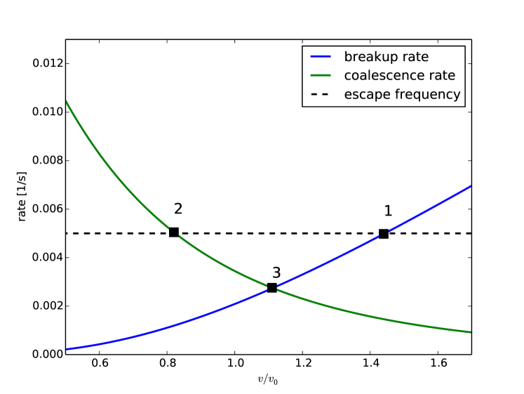
Figure 1: Stable solution to optimization of PBE source terms are located around points indicated with squares. . ‘1’ corresponds to pure breakup solution, ‘2’ is pure coalescence, ‘3’ is balanced solution.

All the above result in an efficient algorithm to optimize steady state solution to population balance equation. Typical convergence rate of optimization is illustrated on Fig. 2.

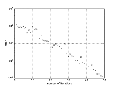
Figure 2: Rate of convergence of optimization process. Left-hand side plot shows error as defined by Eq. 15 as a function of number of iterations. The second plot shows relative change in $C_{1}$–$C_{4}$ parameters being optimized.

3.2 Selected cases

Test case

To validate the methodology and implementation a test case with known analytical solution has been chosen. The selected case is simultaneous breakup and coalescence of polymers from Blatz and Tobolsky (1945). Comparison between solution obtained with transient PBE solver, steady state solution iterated until source term value dropped to $1\text{e-03 }$ of initial value and analytical solution can be seen on Fig. 3. The chosen threshold of $1\text{e-03 }$ is a reasonably good indication of the steady state and an idealized test case can be reproduced with as few as twenty size classes.

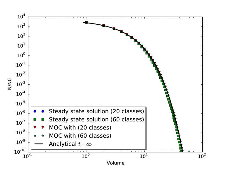
Figure 3: Comparison of steady stat solution, transient solution and analytical result. .

Horizontal pipe flow from Simmons and Azzopardi (2001)

Authors report number of experiments on both upward and horizontal flows of kerosene (continuous phase) and potassium carbonate solution in a $63mm$ pipe. In the paper Sauter mean diameters are reported in three different position in the horizontal systems: bottom, center-line, high position. We choose only one of their cases, with sufficiently high Reynolds number to produce dispersion that is uniform enough to have almost the same mean diameters measured in three different positions. Therefore we take a case with mean flow velocity of $2.71m/s$ and $11.7\%$ of the dispersed phase by volume. For more details we once again refer the reader to the original paper of Simmons and Azzopardi (2001), and for even more detailed description to the thesis of Simmons (1998).

Continuous flow stirred tank from Coulaloglou and Tavlarides (1977)

Experiments were performed in a continuous flow $12l$ baffled stirred tank with a $10cm$ turbine impeller. The liquid-liquid system used was water for the continuous phase and kerosene-dichlorobenzene as the dispersed phase. Non-dimensional numbers governing the flow were calculated based on impeller geometry (as used to describe similar systems for example by Wang and Calabrese (1986); Coulaloglou and Tavlarides (1977)):

$$\mathrm{Re}=\frac{N_{i}D_{i}^{2}}{\mu_{c}\varrho_{c}}$$ (16)

$$\mathrm{Ca}=\frac{\mu_{d}N_{i}D_{i}}{\sigma}\left(\frac{\varrho_{c}}{\varrho_{d}}\right)^{1/2}$$ (17)

$$\mathrm{St}=\frac{2\varrho_{c}}{2\varrho_{d}+\varrho_{c}}\frac{2d_{32}^{2}}{9D_{i}^{2}\beta^{2}}\mathrm{Re}$$ (18)

with $N_{i}$ and $D_{i}$ being, accordingly, impeller speed (in revolutions per second) and impeller diameter. Turbulent kinetic energy dissipation is calculated in the same way as in Coulaloglou and Tavlarides (1977), through formula:

$$\epsilon=0.407aN_{i}^{3}D_{i}^{2}$$ (19)

Horizontal pipe flow from Angeli and Hewitt (2000)

Paper investigates the effect of the pipe material on the droplet size distribution. For the validation we selected six oil(continuous)-water(dispersed) flows in a $24mm$ diameter acrylic pipe.

Horizontal pipe flow from Karabelas (1978)

Author reports oil-water flows in $5.04cm$ diameter pipe at various concentrations from which we select 7 cases.

3.3 Initial conditions

In the fully developed pipe flows the convective term is not taken into account since boundary condition should not effect the result. In cases taken from Coulaloglou and Tavlarides (1977) we take the residence time to be $10min$, exactly the same as reported by the authors.

As an initial distribution for every simulation we take a Gaussian-type function:

$$n_{0}=\frac{\alpha V}{v_{0}}\frac{1}{\sqrt{2\pi}\sigma_{0}}\exp\left(\frac{(v-v_{0})^{2}}{2\sigma_{0}^{2}}\right)$$ (20)

with $v_{0}$ and $\sigma_{0}$ being initial mean volume of drops and their standard deviation and $\alpha$ being volumetric fraction of the dispersed phase in the domain.

case	residence time
Simmons and Azzopardi (2001)	$\infty$
Angeli and Hewitt (2000)	$\infty$
Karabelas (1978)	$\infty$
Coulaloglou and Tavlarides (1977)	$10\text{min}$

Table 1: Residence times used in simulations. Infinite time corresponds to lack of inflow/outflow terms.

4 Results

4.1 Parameter dependency on non-dimensional numbers

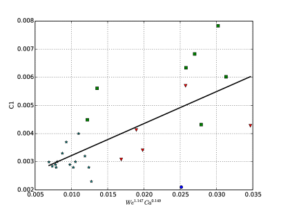
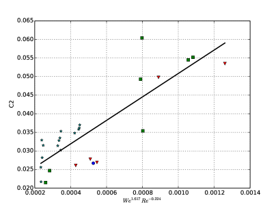
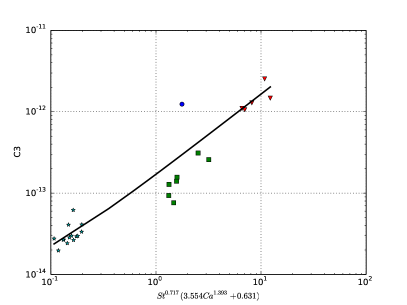
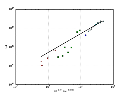
Figure 4: Model parameters together with proposed correlations.

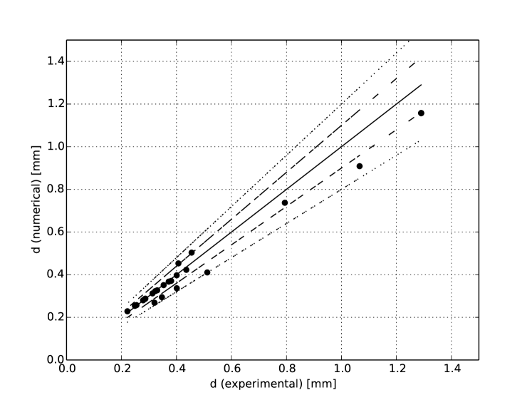
Figure 5: Proposed model predictions versus experimental Sauter mean diameter. Continuous line corresponds to an exact match, dashed lines represent 10% and 20% error accordingly.

Attempt to find the functional dependency on $\mathrm{Re}$, $\mathrm{St}$, $\mathrm{We}$ and $\mathrm{Ca}$ was perform after identification of $C_{1}$ – $C_{4}$ parameters for each case. The $C_{3}$ and $C_{4}$ parameters from coalescence model varied in the selected cases by two orders of magnitude and it is clear that the parameters can be expressed as a function of all important non-dimensional numbers. Their values change monotonically with increasing $\mathrm{Re}$, $\mathrm{St}$, $\mathrm{We}$ and $\mathrm{Ca}$. We propose easy to use correlations expressing the value of coalescence model parameters as a product of non-dimensional groups raised to a certain powers. From least square fitting we find that:

$$C_{3}=1.6429\text{e-13 }\mathrm{St}^{0.7174}\left(3.5541\mathrm{Ca}^{1.3928}+0.6311\right)$$ (21)

$$C_{4}=5.137\text{e08 }\mathrm{St}^{-0.6258}\mathrm{We}^{-0.1874}\mathrm{Re}$$ (22)

The breakup model parameters have not displayed such a clear dependency on chosen non-dimensional numbers since their variation was much smaller than coalescence parameters. There are at least four possible explanations for this situation:

1. functional dependency of $C_{1}$ and $C_{2}$ on flow fields is more complicated than assumed dependency on non-dimensional groups

2. the parameters are constant and the results we obtained can be explained as noisy data scattered around the true value

3. current population balance models do not capture all the essential physics of the problem: either solving population balance equation solved for the whole domain is not accurate enough and using mean dissipation in the domain is not representative or used correlations for breakup and coalescence rates do not take into account all sources of breakup and coalescence events

4. the dependency of $C_{1}$ and $C_{2}$ on the mean flow values is small and uncertainties involved in the approach taken by us prohibit us from identifying it

We choose to treat $C_{1}$ and $C_{2}$ as parameters weakly dependent on several non-dimensional groups that provided best fit with experimental data:

$$C_{1}=0.1137\mathrm{We}^{1.1467}\mathrm{Ca}^{0.1491}+1.0814\text{e-03 }$$ (23)

$$C_{2}=31.56\mathrm{We}^{1.6170}\mathrm{Re}^{-0.2239}+0.01927$$ (24)

Above expression were used to calculate $C_{1}$ – $C_{4}$ values for the final set of simulations and the comparison of obtained mean diameter and experimental values from all 27 simulations are plotted on Fig. 5. We find that most of the results are within 10% error from experimental values and all results fall withing $\pm$20% error band. The results obtained prove that the established model can be successfully applied to number of liquid-liquid flows across a wide range of non-dimensional parameters.

4.2 Recommendations for the future work

Since the physical mechanisms of breakup and coalescence in bubbly flows of other types of dispersed flows are not different from the ones in liquid-liquid flow, similar optimization procedure can be applied to them. It might be possible to find an even more generalized expressions that can be applied for wider range of flows.

Incorporating larger number of experimental cases in the optimization process should result in more reliable correlations also applying the results of this work in a full three-dimensional CFD simulation should help in gaining more confidence in obtained results.

5 Acknowledgements

This work has been undertaken within the Consortium on Transient and Complex Multiphase Flows and Flow Assurance (TMF). The Authors wish to acknowledge the contributions made to this project by the UK Engineering and Physical Sciences Research Council (EPSRC) and the following: - ASCOMP, BPExploration; Cameron Technology & Development; CD-adapco; Chevron; KBC (FEESA); FMC Technologies; INTECSEA; Institutt for Energiteknikk (IFE); Kongsberg Oil & Gas Technologies; MSi Kenny; Petrobras; Schlumberger Information Solutions; Shell; SINTEF; Statoil and TOTAL. The Authors wish to express their sincere gratitude for this support.

References

- Angeli and Hewitt [2000] P. Angeli and G. F. Hewitt. Drop size distributions in horizontal oil-water dispersed flows. Chemical Engineering Science, 55(16):3133–3143, 2000.
- Baldyga and Bourne [1992] J. Baldyga and J. Bourne. Interactions between mixing on various scales in stirred tank reactors. Chemical Engineering Science, 47(8):1839 – 1848, 1992. ISSN 0009-2509. doi: http://dx.doi.org/10.1016/0009-2509(92)80302-S.
- Blatz and Tobolsky [1945] P. Blatz and A. Tobolsky. Note on the kinetics of systems manifesting simultaneous polymerization-depolymerization phenomena. The journal of physical chemistry, 49(2):77–80, 1945.