Multivariate Complexity Analysis of Geometric Red Blue Set Cover

Abstract

We investigate the parameterized complexity of Generalized Red Blue Set Cover (Gen-RBSC), a generalization of the classic Set Cover problem and the more recently studied Red Blue Set Cover problem. Given a universe $U$ containing $b$ blue elements and $r$ red elements, positive integers $k_{\ell}$ and $k_{r}$, and a family $\mathcal{F}$ of $\ell$ sets over $U$, the Gen-RBSC problem is to decide whether there is a subfamily $\mathcal{F}^{\prime}\subseteq\mathcal{F}$ of size at most $k_{\ell}$ that covers all blue elements, but at most $k_{r}$ of the red elements. This generalizes Set Cover  and thus in full generality it is intractable in the parameterized setting. In this paper, we study a geometric version of this problem, called Gen-RBSC-lines, where the elements are points in the plane and sets are defined by lines. We study this problem for an array of parameters, namely, $k_{\ell},k_{r},r,b$, and $\ell$, and all possible combinations of them. For all these cases, we either prove that the problem is W-hard or show that the problem is fixed parameter tractable (FPT). In particular, on the algorithmic side, our study shows that a combination of $k_{\ell}$ and $k_{r}$ gives rise to a nontrivial algorithm for Gen-RBSC-lines. On the hardness side, we show that the problem is para-NP-hard when parameterized by $k_{r}$, and W[1]-hard when parameterized by $k_{\ell}$. Finally, for the combination of parameters for which Gen-RBSC-lines admits FPT algorithms, we ask for the existence of polynomial kernels. We are able to provide a complete kernelization dichotomy by either showing that the problem admits a polynomial kernel or that it does not contain a polynomial kernel unless $\text{co-NP}\subseteq\text{NP}/\mbox{poly}$.

1 Introduction

The input to a covering problem consists of a universe $U$ of size $n$, a family $\mathcal{F}$ of $m$ subsets of $U$ and a positive integer $k$, and the objective is to check whether there exists a subfamily ${\mathcal{F^{\prime}}}\subseteq{\mathcal{F}}$ of size at most $k$ satisfying some desired properties. If ${\cal F}^{\prime}$ is required to contain all the elements of $U$, then it corresponds to the classical Set Cover problem. The Set Cover problem is part of Karp’s $21$ NP-complete problems [13]. This, together with its numerous variants, is one of the most well-studied problems in the area of algorithms and complexity. It is one of the central problems in all the paradigms that have been established to cope with NP-hardness, including approximation algorithms, randomized algorithms and parameterized complexity.

1.1 Problems Studied, Context and Framework

The goal of this paper is to study a generalization of a variant of Set Cover  namely, the Red Blue Set Cover problem.

Red Blue Set Cover (RBSC) Input: A universe $U=(R,B)$ where $R$ is a set of $r$ red elements and $B$ is a set of $b$ blue elements, a family $\mathcal{F}$ of $\ell$ subsets of $U$, and a positive integer $k_{r}$. Question: Is there a subfamily ${\mathcal{F}^{\prime}}$ of sets that covers all blue elements but at most $k_{r}$ red elements?

Red Blue Set Cover was introduced in 2000 by Carr et al. [2]. This problem is closely related to several combinatorial optimization problems such as the Group Steiner, Minimum Label Path, Minimum Monotone Satisfying Assignment and Symmetric Label Cover problems. This has also found applications in areas like fraud/anomaly detection, information retrieval and the classification problem. Red Blue Set Cover  is NP-complete, following from an easy reduction from Set Cover itself.

In this paper, we study the parameterized complexity, under various parameters, of a common generalization of both Set Cover and Red Blue Set Cover, in a geometric setting.

Generalized Red Blue Set Cover (Gen-RBSC) Input: A universe $U=(R,B)$ where $R$ is a set of $r$ red elements and $B$ is a set of $b$ blue elements, a family $\mathcal{F}$ of $\ell$ subsets of $U$, and positive integers $k_{\ell},k_{r}$. Question: Is there a subfamily ${\mathcal{F}^{\prime}}\subseteq\mathcal{F}$ of size at most $k_{\ell}$ that covers all blue elements but at most $k_{r}$ red elements?

It is easy to see that when $k_{\ell}=|\mathcal{F}|$ then the problem instance is a Red Blue Set Cover instance, while it is a Set Cover instance when $k_{\ell}=k,R=\emptyset,k_{r}=0$. Next we take a short detour and give a few essential definitions regarding parameterized complexity.

Parameterized complexity. The goal of parameterized complexity is to find ways of solving NP-hard problems more efficiently than brute force: here the aim is to restrict the combinatorial explosion to a parameter that is hopefully much smaller than the input size. Formally, a parameterization of a problem is assigning a positive integer parameter $k$ to each input instance and we say that a parameterized problem is fixed-parameter tractable (FPT) if there is an algorithm that solves the problem in time $f(k)\cdot|I|^{\mathcal{O}(1)}$, where $|I|$ is the size of the input and $f$ is an arbitrary computable function depending only on the parameter $k$. Such an algorithm is called an FPT algorithm and such a running time is called FPT running time. There is also an accompanying theory of parameterized intractability using which one can identify parameterized problems that are unlikely to admit FPT algorithms. These are essentially proved by showing that the problem is W-hard. A parameterized problem is said to admit a $h(k)$-kernel if there is a polynomial time algorithm (the degree of the polynomial is independent of $k$), called a kernelization algorithm, that reduces the input instance to an instance with size upper bounded by $h(k)$, while preserving the answer. If the function $h(k)$ is polynomial in $k$, then we say that the problem admits a polynomial kernel. While positive kernelization results have appeared regularly over the last two decades, the first results establishing infeasibility of polynomial kernels for specific problems have appeared only recently. In particular, Bodlaender et al. [1], and Fortnow and Santhanam [11] have developed a framework for showing that a problem does not admit a polynomial kernel unless $\text{co-NP}\subseteq\text{NP}/\mbox{poly}$, which is deemed unlikely. For more background, the reader is referred to the following monograph [9].

In the parameterized setting, Set Cover, parameterized by $k$, is W[2]-hard [7] and it is not expected to have an FPT algorithm. The NP-hardness reduction from Set Cover to Red Blue Set Cover implies that Red Blue Set Cover is W[2]-hard parameterized by the size $k_{\ell}$ of a solution subfamily. However, the hardness result was not the end of the story for the Set Cover problem in parameterized complexity. In literature, various special cases of Set Cover have been studied. A few examples are instances with sets of bounded size [8], sets with bounded intersection [15, 20], and instances where the bipartite incidence graph corresponding to the set family has bounded treewidth or excludes some graph $H$ as a minor [4, 10]. Apart from these results, there has also been extended study on different parameterizations of Set Cover. A special case of Set Cover  which is central to the topic of this paper is the one where the sets in the family correspond to some geometric object. In the simplest geometric variant of Set Cover, called Point Line Cover, the elements of $U$ are points in ${\mathbb{R}}^{2}$ and each set contains a maximal number of collinear points. This version of the problem is FPT and in fact has a polynomial kernel [15]. Moreover, the size of these kernels have been proved to be tight, under standard assumptions, in [14]. When we take the sets to be the space bounded by unit squares, Set Cover  is W[1]-hard [16]. On the other hand when surfaces of hyperspheres are sets then the problem is FPT [15]. There are several other geometric variants of Set Cover that have been studied in parameterized complexity, under the parameter $k$, the size of the solution subfamily. These geometric results motivate a systematic study of the parameterized complexity of geometric Gen-RBSC problems.

There is an array of natural parameters in hand for the Gen-RBSC problem. Hence, the problem promises an interesting dichotomy in parameterized complexity, under the various parameters. In this paper, we concentrate on the Generalized Red Blue Set Cover with lines problem, parameterized under combinations of natural parameters.

Generalized Red Blue Set Cover with lines (Gen-RBSC-lines) Input: A universe $U=(R,B)$ where $R$ is a set of $r$ red points and $B$ is a set of $b$ blue points, a family $\mathcal{F}$ of $\ell$ sets of $U$ such that each set contains a maximal set of collinear points of $U$, and positive integers $k_{\ell},k_{r}$. Question: Is there a subfamily ${\mathcal{F}^{\prime}}\subseteq\mathcal{F}$ of size at most $k_{\ell}$ that covers all blue points but at most $k_{r}$ red points?

It is safe to assume that $r\geq k_{r}$, and $\ell\geq k_{\ell}$. Since it is enough to find a minimal solution family $\mathcal{F}^{\prime}$, we can also assume that $b\geq k_{\ell}$.

We finish this section with some related results. As mentioned earlier, the Red Blue Set Cover problem in classical complexity is NP-complete. Interestingly, if the incidence matrix, built over the sets and elements, has the consecutive ones property then the problem is in $P$ [5]. The problem has been studied in approximation algorithms as well [2, 19]. Specially, the geometric variant, where every set is the space bounded by a unit square, has a polynomial time approximation scheme (PTAS) [3].

1.2 Our Contributions

In this paper, we first show a complete dichotomy of the parameterized complexity of Gen-RBSC-lines. For a list of parameters, namely, $k_{\ell},k_{r},r,b$, and $\ell$, and all possible combinations of them, we show hardness or an FPT algorithm. Further, for parameterizations where an FPT algorithm exists, we either show that the problem admits a polynomial kernel or that it does not contain a polynomial kernel unless $\text{co-NP}\subseteq\text{NP}/\mbox{poly}$.

To describe our results we first state a few definitions. For a set $S\subseteq U$, we denote by $2^{S}$ the family of all the subsets of $S$, and by $U^{S}$ the family of all the subsets of $U$ that contain $S$ (that is, all supersets of $S$ in $U$). For a collection $\mathfrak{F}$ of sets over a universe $U$, by ${\sf DownClosure}(\mathfrak{F})$ and ${\sf UpClosure}(\mathfrak{F})$ we mean the families $\bigcup_{S\in\mathfrak{F}}2^{S}\mbox{ and }\bigcup_{S\in\mathfrak{F}}U^{S}$ respectively. Our first contribution is the following parameterized and kernelization dichotomy result for Gen-RBSC-lines.

Theorem 1.1.

Let $\Gamma=\{\ell,r,b,k_{\ell},k_{r}\}$. Then Gen-RBSC-lines is FPT  parameterized by $\Gamma^{\prime}\subseteq\Gamma$ if and only if $\Gamma^{\prime}\notin{\sf DownClosure}(\{\{k_{\ell},b\},\{r\}\})$. Furthermore, Gen-RBSC-lines admits a polynomial kernel parameterized by $\Gamma^{\prime}\subseteq\Gamma$ if and only if $\Gamma^{\prime}\in{\sf UpClosure}(\{\{\ell\},\{k_{\ell},r\},\{b,r\}\})$.

Essentially, the theorem says that if Gen-RBSC-lines is FPT  parameterized by $\Gamma^{\prime}\subseteq\Gamma$ then there exists an algorithm for Gen-RBSC-lines running in time $f(\Gamma^{\prime})\cdot(|U|+|{\cal F}|)^{\mathcal{O}(1)}$. That is, the running time of the algorithm can depend in an arbitrary manner on the parameters present in $\Gamma^{\prime}$. Equivalently, we have an algorithm running in time $f(\tau)\cdot(|U|+|{\cal F}|)^{\mathcal{O}(1)}$, where $\tau=\sum_{q\in\Gamma^{\prime}}q$. Similarly, if the problem admits a polynomial kernel parameterized by $\Gamma^{\prime}$ then in polynomial time we get an equivalent instance of the problem of size $\tau^{\mathcal{O}(1)}$. On the other hand when we say that the problem does not admit polynomial kernel parameterized by $\Gamma^{\prime}$ then it means that there is no kernelization algorithm outputting a kernel of size $\tau^{\mathcal{O}(1)}$ unless $\text{co-NP}\subseteq\text{NP}/\mbox{poly}$. A schematic diagram explaining the results proved in Theorem 1.1 can be seen in Figure 1. Results for a $\Gamma^{\prime}\subseteq\Gamma$ which is not depicted in Figure 1 can be derived by checking whether $\Gamma^{\prime}$ is in ${\sf DownClosure}(\{\{k_{\ell},b\},\{r\}\})$.

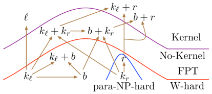
Figure 1: Illustration of our results described in Theorem 1.1 and hierarchy of parameters.

Next we consider the RBSC-lines problem. Here we do not have any constraint on how many sets we pick in the solution family but we are allowed to cover at most $k_{r}$ red points. This brings two main changes in Figure 1. For Gen-RBSC-lines we show that the problem is NP-hard even when there is a constant number of red points. However, RBSC-lines becomes FPT parameterized by $r$. In contrast, RBSC-lines is W[1]-hard parameterized by $k_{r}$. This leads to the following dichotomy theorem for RBSC-lines.

Theorem 1.2.

Let $\Gamma=\{\ell,r,b,k_{r}\}$. Then RBSC-lines is FPT  parameterized by $\Gamma^{\prime}\subseteq\Gamma$ if and only if $\Gamma^{\prime}\notin\{\{b\},\{k_{r}\}\})$. Furthermore, RBSC-lines admits polynomial kernel parameterized by $\Gamma^{\prime}\subseteq\Gamma$ if and only if $\Gamma^{\prime}\in{\sf UpClosure}(\{\{\ell\},\{b,r\}\})$.

A schematic diagram explaining the results proved in Theorem 1.2 is given in Figure 2.

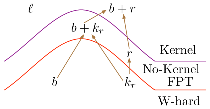
Figure 2: Illustration of our results for Red Blue Set Cover with lines under various parameters.

A quick look at Figure 1 will show that the Gen-RBSC-lines problem is FPT  parameterized by $k_{\ell}+k_{r}$ or $b+k_{r}$. A natural question to ask is whether Gen-RBSC itself (the problem where sets in the input family are arbitrary and do not correspond to lines) is FPT when parameterized by $b+k_{r}$. Regarding this, we show the following results:

1. Gen-RBSC is W[1]-hard parameterized by $k_{\ell}+k_{r}$ (or $b+k_{r}$) when every set has size at most three and contains at least two red points.

2. Gen-RBSC is W[2]-hard parameterized by $k_{\ell}+r$ when every set contains at most one red point.

The first result essentially shows that Gen-RBSC  is W[1]-hard even when the sets in the family has size bounded by three. This is in sharp contrast to Set Cover, which is known to be FPT parameterized by $k_{\ell}$ and $d$. Here, $d$ is the size of the maximum cardinality set in $\cal F$. In fact, Set Cover admits a kernel of size $k_{\ell}^{\mathcal{O}(d)}$. This leads to the following question:

Does the hardness of Gen-RBSC in item one arise from the presence of two red points in the instance? Would the complexity change if we assume that each set contains at most one red point?

In fact, even if we assume that each set contains at most one red point, we must take $d$, the size of the maximum cardinality set in $\cal F$, as a parameter. Else, this would correspond to the hardness result presented in item two. As a final algorithmic result we show that Gen-RBSC admits an algorithm with running time $2^{\mathcal{O}(dk_{\ell})}\cdot(|U|+|{\cal F}|)^{\mathcal{O}(1)}$, when every set has at most one red point. Observe that in this setting $k_{r}$ can always be assumed to be less than $k_{\ell}$. Thus, this is also a FPT algorithm parameterized by $k_{\ell}+k_{r}$, when sets in the input family are bounded. However, we show that Gen-RBSC  (in fact Gen-RBSC-lines) does not admit a polynomial kernel parameterized by $k_{\ell}+k_{r}$ even when each set in the input family corresponds to a line and has size two and contains at most one red point.

1.3 Our methods and an overview of main algorithmic results

Let $\Gamma=\{\ell,r,b,k_{\ell},k_{r}\}$. Most of our W-hardness results for a Gen-RBSC variant parameterized by $\Gamma^{\prime}\subseteq\Gamma$ are obtained by giving a polynomial time reduction, from Set Cover or Multicolored Clique  that makes every $q\in\Gamma^{\prime}$ at most $k^{\mathcal{O}(1)}$ (in fact most of the time $\mathcal{O}(k)$). This allows us to transfer the known hardness results about Set Cover and Multicolored Clique to our problem. Since in most cases the parameters are linear in the input parameter, in fact we can rule out an algorithm of form $(|U|+|{\cal F}|)^{o(\tau)}$, where $\tau=\sum_{q\in\Gamma^{\prime}}q$, under Exponential Time Hypothesis (ETH) [12]. Similarly, hardness results for kernels are derived from giving an appropriate polynomial time reduction from parameterized variants of the Set Cover problem that only allows each parameter $q\in\Gamma^{\prime}$ to grow polynomially in the input parameter.

Our main algorithmic highlights are parameterized algorithms for

1. Gen-RBSC-lines  running in time $2^{\mathcal{O}(k_{\ell}\log k_{\ell}+k_{r}\log k_{r})}\cdot(|U|+|{\cal F}|)^{\mathcal{O}(1)}$ (showing Gen-RBSC-lines  is FPT parameterized by $k_{\ell}+k_{r}$); and

2. Gen-RBSC with running time $2^{\mathcal{O}(dk_{\ell})}\cdot(|U|+|{\cal F}|)^{\mathcal{O}(1)}$, when every set is of size at most $d$ and has at most one red point.

Observe that the first algorithm generalizes the known algorithm for Point Line Cover which runs in time $2^{\mathcal{O}(k_{\ell}\log k_{\ell})}\cdot(|U|+|{\cal F}|)^{\mathcal{O}(1)}$ [15].

The parameterized algorithm for Gen-RBSC-lines mentioned in (a) starts by bounding the number of blue vertices by $k_{\ell}^{2}$ and guessing the lines that contain at least two blue points. The number of lines containing at least two blue points can be shown to be at most $k_{\ell}^{4}$. These guesses lead to an equivalent instance where each line contains exactly one blue point and there are no lines that only contain red points (as these lines can be deleted). However, we can not bound the number of red points at this stage. We introduce a notion of ”solution subfamily” and connected components of the solution subfamilies. Interestingly, this equivalent instance has sufficient geometric structure on the connected components. We exploit the structure of these components, gotten mainly from simple properties of lines on a plane, to show that knowing one of the lines in each component can, in FPT time, lead to finding the component itself! Thus, to find a component all we need to do is to guess one of the lines in it. However, here we face our second difficulty: the number of connected components can be as bad as $\mathcal{O}(k_{\ell})$ and thus if we guess one line for each connected component then it would lead to a factor of $|{\cal F}|^{\mathcal{O}(k_{\ell})}$ in the running time of the algorithm. However, our equivalent instances are such that we are allowed to process each component independent of other components. This brings the total running time of guessing the first line of each component down to $k_{\ell}\cdot|{\cal F}|$. The algorithmic ideas used here can be viewed as some sort of “geometry preserving subgraph isomorphism”, which could be useful in other contexts also. This completes an overview of the FPT result for Gen-RBSC-lines parameterized by $k_{\ell}+k_{r}$.

The algorithm for Gen-RBSC  running in time $2^{\mathcal{O}(dk_{\ell})}\cdot(|U|+|{\cal F}|)^{\mathcal{O}(1)}$, where every set is of size at most $d$ and has at most one red point is purely based on a novel reduction to Subgraph Isomorphism where the subgraph we are looking for has size $\mathcal{O}(k_{\ell}d)$ and treewidth $3$. The host graph, where we are looking for a solution subgraph, is obtained by starting with the bipartite incidence graph and making modifications to it. The bipartite incidence graph we start with has in one side vertices for sets and in the other side vertices corresponding to blue and red points and there is an edge between vertices corresponding to a set and a blue (red) point if this blue (red) point is contained in the set. Our main observation is that a solution subfamily can be captured by a subgraph of size $\mathcal{O}(k_{\ell}d)$ and treewidth $3$. Thus, for our algorithm we enumerate all such subgraphs in time $2^{\mathcal{O}(dk_{\ell})}\cdot(|U|+|{\cal F}|)^{\mathcal{O}(1)}$ and for each such subgraph we check whether it exists in the host graph using known algorithms for Subgraph Isomorphism. This concludes the description of this algorithm.

2 Preliminaries

In this paper an undirected graph is denoted by a tuple $G=(V,E)$, where $V$ denotes the set of vertices and $E$ the set of edges. For a set $S\subseteq V$, the subgraph of $G$ induced by $S$, denoted by $G[S]$, is defined as the subgraph of $G$ with vertex set $S$ and edge set $\{(u,v)\in E:u,v\in S\}$. The subgraph obtained after deleting $S$ is denoted as $G\setminus S$. All vertices adjacent to a vertex $v$ are called neighbors of $v$ and the set of all such vertices is called the neighborhood of $v$. Similarly, a non-adjacent vertex of $v$ is called a non-neighbor and the set of all non-neighbors of $v$ is called the non-neighborhood of $v$. The neighborhood of $v$ is denoted by $N(v)$. A vertex in a connected graph is called a cut vertex if its deletion results in the graph becoming disconnected.

Recall that showing a problem W[1] or W[2] hard implies that the problem is unlikely to be FPT. One can show that a problem is W[1]-hard (W[2]-hard) by presenting a parameterized reduction from a known W[1]-hard problem (W[2]-hard) such as Clique (Set Cover) to it. The most important property of a parameterized reduction is that it corresponds to an FPT algorithm that bounds the parameter value of the constructed instance by a function of the parameter of the source instance. A parameterized problem is said to be in the class para-NP if it has a nondeterministic algorithm with FPT running time. To show that a problem is para-NP-hard we need to show that the problem is NP-hard for some constant value of the parameter. For an example $3$-Coloring is para-NP-hard parameterized by the number of colors. See [9] for more details.

Lower bounds in Kernelization. In the recent years, several techniques have been developed to show that certain parameterized problems belonging to the FPT class cannot have any polynomial sized kernel unless some classical complexity assumptions are violated. One such technique that is widely used is the polynomial parameter transformation technique.

Definition 1.

Let $\Pi,\Gamma$ be two parameterized problems. A polynomial time algorithm $\mathcal{A}$ is called a polynomial parameter transformation (or ppt) from $\Pi$ to $\Gamma$ if , given an instance $(x,k)$ of $\Pi$, $\mathcal{A}$ outputs in polynomial time an instance $(x^{\prime},k^{\prime})$ of $\Gamma$ such that $(x,k)\in\Pi$ if and only if $(x^{\prime},k^{\prime})\in\Gamma$ and $k^{\prime}\leq p(k)$ for a polynomial $p$.

We use the following theorem together with ppt reductions to rule out polynomial kernels.

Theorem 2.1.

Let $\Pi,\Gamma$ be two parameterized problems such that $\Pi$ is NP-hard and $\Gamma\in\text{NP}$. Assume that there exists a polynomial parameter transformation from $\Pi$ to $\Gamma$. Then, if $\Pi$ does not admit a polynomial kernel neither does $\Gamma$.

For further details on lower bound techniques in kernelization refer to [1, 11].

Generalized Red Blue Set Cover. A set $S$ in an Generalized Red Blue Set Cover instance $(U,\mathcal{F})$ is said to cover a point $p\in U$ if $p\in S$. A solution family for the instance is a family of sets of size at most $k_{\ell}$ that covers all the blue points and at most $k_{r}$ red points. In case of Red Blue Set Cover, the solution family is simply a family of sets that covers all the blue points but at most $k_{r}$ red points. Such a family will also be referred to as a valid family. A minimal family of sets is a family of sets such that every set contains a unique blue point. In other words, deleting any set from the family implies that a strictly smaller set of blue points is covered by the remaining sets. The sets of Generalized Red Blue Set Cover with lines are also called lines in this paper. We also mention a key observation about lines in this section. This observation is crucial in many arguments in this paper.

Observation 1.

Given a set of points $S$, let $\mathcal{F}$ be the set of lines such that each line contains at least $2$ points from $S$. Then $|\mathcal{F}|\leq{|S|\choose 2}$.

Gen-RBSC with hyperplanes of ${\mathbb{R}}^{d}$, for a fixed positive integer $d$, is a special case for the problem. Here, the input universe $U$ is a set of $n$ points in ${\mathbb{R}}^{d}$. A hyperplane in ${\mathbb{R}}^{d}$ is the affine hull of a set of $d+1$ affinely independent points [15]. In our special case each set is a maximal set of points that lie on a hyperplane of ${\mathbb{R}}^{d}$.

Definition 2.

An intersection graph $G_{\mathcal{F}}=(V,E)$ for an instance $(U,\mathcal{F})$ of Generalized Red Blue Set Cover is a graph with vertices corresponding to the sets in $\mathcal{F}$. We give an edge between two vertices if the corresponding sets have non-empty intersection.

The following proposition is a collection of results on the Set Cover problem, that will be repeatedly used in the paper. The results are from [6, 7]

Proposition 1.

The Set Cover problem is:

1. W[2] hard when parameterized by the solution family size $k$.

2. FPT when parameterized by the universe size $n$, but does not admit polynomial kernels unless $\text{co-NP}\subseteq\text{NP}/\mbox{poly}$.

3. FPT when parameterized by the number of sets $m$ in the instance, but does not admit polynomial kernels unless $\text{co-NP}\subseteq\text{NP}/\mbox{poly}$.

Tree decompositions and treewidth. We also need the concept of treewidth and tree decompositions.

Definition 3 (Tree Decomposition  [21]).

A tree decomposition of a (undirected or directed) graph $G=(V,E)$ is a tree $\mathbb{T}$ in which each vertex $x\in\mathbb{T}$ has an assigned set of vertices $B_{x}\subseteq V$ (called a bag) such that $(\mathbb{T},\{B_{x}\}_{x\in\mathbb{T}})$ has the following properties:

• $\bigcup_{x\in\mathbb{T}}B_{x}=V$

• For any $(u,v)\in E$, there exists an $x\in\mathbb{T}$ such that $u,v\in B_{x}$.

• If $v\in B_{x}$ and $v\in B_{y}$, then $v\in B_{z}$ for all $z$ on the path from $x$ to $y$ in $\mathbb{T}$.

In short, we denote $(\mathbb{T},\{B_{x}\}_{x\in\mathbb{T}})$ as $\mathbb{T}$.

The treewidth $tw(\mathbb{T})$ of a tree decomposition $\mathbb{T}$ is the size of the largest bag of $\mathbb{T}$ minus one. A graph may have several distinct tree decompositions. The treewidth $tw(G)$ of a graph $G$ is defined as the minimum of treewidths over all possible tree decompositions of $G$.

3 Parameterizing by $k_{r}$ and $r$

In this section we first show that Gen-RBSC-lines parameterized by $r$ is para-NP-complete. Since $k_{r}\leq r$, it follows that Gen-RBSC-lines parameterized by $k_{r}$ is also para-NP-complete.

Theorem 3.1.

Gen-RBSC-lines is para-NP-complete parameterized by either $r$ or $k_{r}$.

Proof.

If we are given a solution family for an instance of Gen-RBSC-lines we can check in polynomial time if it is valid. Hence, Gen-RBSC-lines  has a nondeterministic algorithm with FPT running time (in fact polynomial) and thus Gen-RBSC-lines  parameterized by $r$ is in para-NP.

For completeness, there is an easy polynomial-time many-one reduction from the Point Line Cover problem, which is NP-complete. An instance $((U,\mathcal{F}))$ of Point Line Cover parameterized by $k$, the size of the solution family, is reduced to an instance $((R\cup B,\mathcal{F}))$ of Gen-RBSC-lines parameterized by $r$ or $k_{r}$ with the following properties:

• $B=U$

• The family of sets remains the same in both instances.

• $R$ consists of $1$ red vertex that does not belong to any of the lines of $\mathcal{F}$.

• $k_{\ell}=k$ and $k_{r}=0$.

It is easy to see that $((U,\mathcal{F}))$ is a YES instance of Point Line Cover if and only if $(R\cup B,\mathcal{F})$ is a YES instance of Gen-RBSC-lines. Since the reduced instances belong to Gen-RBSC-lines parameterized by $r=1$ or $k_{r}=0$, this proves that Gen-RBSC-lines parameterized by $r$ or $k_{r}$ is para-NP-complete. ∎

4 Parameterizing by $\ell$

In this section we design a parameterized algorithm as well as a kernel for Gen-RBSC-lines when parameterized by the size $\ell$ of the family. The algorithm for this is simple. We enumerate all possible $k_{\ell}$-sized subsets of input lines and for each subset, we check in polynomial time whether it covers all blue points and at most $k_{r}$ red points. The algorithm runs in time $\mathcal{O}(2^{\ell}\cdot(|U|+|\mathcal{F}|)$. The main result of this section is a polynomial kernel for Gen-RBSC-lines when parameterized by $\ell$.

We start by a few reduction rules which will be used not only in the kernelization algorithm given below but also in other parameterized and kernelization algorithms in subsequent sections.

Reduction Rule 1.

If there is a set $S\in\mathcal{F}$ with only red points then delete $S$ from $\mathcal{F}$.

Lemma 4.1.

Reduction Rule 1 is safe.

Proof.

Let $\mathcal{F}^{\prime}$ be a family of at most $k_{\ell}$ lines of the given instance that cover all blue points and at most $k_{r}$ red points. If $\mathcal{F}^{\prime}$ contains $S$, then $\mathcal{F}^{\prime}\setminus\{S\}$ is also a family of at most $k_{\ell}$ lines that cover all blue points and at most $k_{r}$ red points. Hence, we can safely delete $S$. This shows that Reduction Rule 1 is safe. ∎

Reduction Rule 2.

If there is a set $S\in\mathcal{F}$ with more than $k_{r}$ red points in it then delete $S$ from $\mathcal{F}$.

Lemma 4.2.

Reduction Rule 2 is safe.

Proof.

If $S$ has more than $k_{r}$ red points then $S$ alone exceeds the budget given for the permissible number of covered red points. Hence, $S$ cannot be part of any solution family and can be safely deleted from the instance. This shows that Reduction Rule 2 is safe. ∎

Our final rule is as follows. A similar Reduction Rule was used in [15], for the Point Line Cover problem.

Reduction Rule 3.

If there is a set $S\in\mathcal{F}$ with at least $k_{\ell}+1$ blue points then reduce the budget of $k_{\ell}$ by $1$ and the budget of $k_{r}$ by $|R\cap S|$. The new instance is $(U\setminus S,\widetilde{{\cal F}})$, where $\widetilde{{\cal F}}=\{F\setminus S~{}|~{}F\in{\cal F}\mbox{ and }F\neq S\}$.

Lemma 4.3.

Reduction Rule 3 is safe.

Proof.

If $S$ is not part of the solution family then we need at least $k_{\ell}+1$ lines in the solution family to cover the blue points in $S$, which is not possible. Hence any solution family must contain $S$.

Suppose the reduced instance has a solution family $\mathcal{F}^{\prime}$ covering $B\setminus S$ blue points and at most $k_{r}-|R\cap S|$ red points from $R\setminus S$. Then $\mathcal{F}^{\prime}\cup\{S\}$ is a solution for the original instance. On the other hand, suppose the original instance has a solution family $\hat{\mathcal{F}}$. As argued above, $S\in\hat{\mathcal{F}}$. $\hat{\mathcal{F}}\setminus S$ covers all blue points of $B\setminus S$ and at most $k_{r}-|R\cap S|$ red points from $R\setminus S$, and is a candidate solution family for the reduced instance. Thus, Reduction Rule 3 is safe. ∎

The following simple observation can be made after exhaustive application of Reduction Rule 3.

Observation 2.

If the budget for the subfamily $\mathcal{F}^{\prime}$ to cover all blue and at most $k_{r}$ red points is $k_{\ell}$ then after exhaustive applications of Reduction Rule 3 there can be at most $b\leq k_{\ell}^{2}$ blue points remaining in a YES instance. If there are more than $k_{\ell}^{2}$ blue points remaining to be covered then we correctly say NO.

It is worth mentioning that even if we had weights on the red points in $R$ and asked for a solution family of size at most $k_{\ell}$ that covered all blue points but red points of weight at most $k_{r}$, then this weighted version, called Weighted Gen-RBSC-lines parameterized by $\ell$ is FPT. The Weighted Gen-RBSC-lines problem will be useful in the theorem below. Finally, we get the following result.

Theorem K.1.

There is an algorithm for Gen-RBSC-lines  running in time $\mathcal{O}(2^{\ell}\cdot(|U|+|\mathcal{F}|))$. In fact, Gen-RBSC-lines  admits a polynomial kernel parameterized by $\ell$.

Proof.

We have already described the enumeration based algorithm at the beginning of this section. Here, we only give the polynomial kernel. Given an instance of Gen-RBSC-lines we exhaustively apply Reduction Rules 1, 2 and 3 to obtain an equivalent instance. By Observation 2 and the fact that $k_{\ell}\leq\ell$, the current instance must have at most $\ell^{2}$ blue points, or we can safely say NO. Also, the number of red points that belong to $2$ or more lines is bounded by the number of intersection points of the $\ell$ lines, i.e., $\ell^{2}$. Any remaining red points belong to exactly $1$ line. We reduce our Gen-RBSC-lines instance to a Weighted Gen-RBSC-lines instance as follows:

• The family of lines and the set of blue points remain the same in the reduced instance. The red points appearing in the intersection of two lines also remain the same. Give a weight of $1$ to these red points.

• For each line $L$, let $c(L)$ indicate the number of red points that belong exclusively to $L$. Remove all but one of these red points and give weight $c(L)$ to the remaining exclusive red point.

In the Weighted Gen-RBSC-lines instance, there are $\ell$ lines, at most $\ell^{2}$ blue points and at most $\ell^{2}+\ell$ red points. For each line $L$, the value of $c(L)$ is at most $k_{r}$, after Reduction Rule 2. Suppose $k_{r}>2^{\ell}$. Then $r>2^{\ell}$ and the parameterized algorithm for Gen-RBSC-lines  running in time $\mathcal{O}(2^{\ell}\cdot(|U|+|\mathcal{F}|))$ runs in polynomial time. Thus we can assume that $k_{r}\leq 2^{\ell}$. Then we can represent $k_{r}$ and therefore the weights $c(L)$ by at most $\ell$ bits. Thus, the reduced instance has size bounded by $\mathcal{O}(\ell^{2})$.

Observe that we got an instance of Weighted Gen-RBSC-lines and not of Gen-RBSC-lines  which is the requirement for the kernelization procedure. All this shows is that the reduction is a “compression” from Gen-RBSC-lines parameterized by $\ell$ to Weighted Gen-RBSC-lines parameterized by $\ell$. This is rectified as follows. Since both the problems belong to NP, there is a polynomial time many-one reduction from Weighted Gen-RBSC-lines to Gen-RBSC-lines. Finally, using this polynomial time reduction, we obtain a polynomial size kernel for Gen-RBSC-lines parameterized by $\ell$. ∎

Observe that the algorithm referred to in Theorem K.1 does not use the fact that sets are lines and thus it also works for Gen-RBSC parameterized by $\ell$. However, it follows from Proposition 1(iii) that Gen-RBSC parameterized by $\ell$ does not admit a polynomial kernel.

5 Parameterizing by $k_{\ell}$, $b$ and $k_{\ell}+b$

In this section we look at Gen-RBSC-lines parameterized by $k_{\ell}$, $b$, and $k_{\ell}+b$. There is an interesting connection between $b$ and $k_{\ell}$. As we are looking for minimal solution families, we can alway assume that $b\geq k_{\ell}$. On the other hand, Reduction Rule 3 showed us that for all practical purposes $b\leq k_{\ell}^{2}$. Thus, in the realm of parameterized complexity $k_{\ell}$, $b$ and $k_{\ell}+b$ are the same parameters. That is, Gen-RBSC-lines is FPT parameterized by $k_{\ell}$ if and only if it is FPT parameterized by $b$ if and only if it is FPT parameterized by $k_{\ell}+b$. The same holds in the context of kernelization complexity. First, we show that Gen-RBSC-lines parameterised by $k_{\ell}$ or $b$ is W[1]-hard. Then we look at some special cases that turn out to be FPT.

5.1 Parameter $k_{\ell}+b$

We look at Gen-RBSC-lines parameterized by $k_{\ell}+b$. This problem is not expected to have a FPT algorithm as it is W[1]-hard. We give a reduction to this problem from the Multicolored Clique problem, which is known to be W[1] hard even on regular graphs [18].

Multicolored Clique Parameter: $k$ Input: A graph $G=(V,E)$ where $V=V_{1}\uplus V_{2}\uplus\ldots\uplus V_{k}$ with $V_{i}$ being an independent set for all $1\leq i\leq k$, and an integer $k$. Question: Is there a clique $C\subseteq G$ of size $k$ such that $\forall 1\leq i\leq k,C\cap V_{i}\neq\emptyset$.

The clique containing one vertex from each part is called a multi-colored clique.

Theorem 5.1.

Gen-RBSC-lines parameterized by $k_{\ell}$ or $b$ or $k_{\ell}+b$ is W[1]-hard.

Proof.

We will give a reduction from Multicolored Clique on regular graphs. Let $(G=(V,E),k)$ be an instance of Multicolored Clique, where $G$ is a $d$-regular graph. We construct an instance of Gen-RBSC-lines  $(R\cup B,\mathcal{F})$, as follows. Let $V=V_{1}\uplus V_{2}\uplus\ldots\uplus V_{k}$.

1. For each vertex class $V_{i},1\leq i\leq k$, add two blue points $b_{i}$ at $(0,i)$ and $b^{\prime}_{i}$ at $(i,0)$.

2. Informally, for each vertex class $V_{i},1\leq i\leq k$ we do as follows. Let $L_{k}$ be the line that is parallel to $y$ axis and passes through the point $(k,0)$. Suppose there are $n_{i}$ vertices in $V_{i}$. We select $n_{i}$ distinct points, say ${\cal P}$, in ${\mathbb{R}}^{2}$ on the line $L$, such that if $(a_{i},a_{2})\in\cal P$ then $a_{i}=k$ (as these are points on $L_{k}$) and $a_{2}$ lies in the interval $(i-1,i-\frac{1}{2})$. Now for every point $p\in\cal P$ we draw the unique line between $(0,i)$ and the point $p$. Finally, we assign each line to a unique vertex in $V_{i}$. Formally, we do as follows. For each vertex class $V_{i},1\leq i\leq k$ and each vertex $u\in V_{i}$, we choose a point $p^{1}_{u}\in{\mathbb{R}}^{2}$ with coordinates $(k,y_{u})$, $i-1<y_{u}<i-\frac{1}{2}$. Also, for each pair $u\neq v\ \in V_{i}$, $y_{u}\neq y_{v}$. For each $u\in V_{i}$, we add the line $l^{1}_{u}$, defined by $b_{i}$ and $p^{1}_{u}$, to $\mathcal{F}$. We call these near-horizontal lines. Observe that all the near-horizontal lines corresponding to vertices in $V_{i}$ intersect at $b_{i}$. Furthermore, for any two vertices $u\in V_{i}$ and $v\in V_{j}$, with $i\neq j$, the lines $l^{1}_{u}$ and $l^{1}_{v}$ do not intersect on a point with $x$-coordinate from the closed interval $[0,k]$.

3. Similarly, for each vertex class $V_{i},1\leq i\leq k$ and each vertex $u\in V_{i}$, we choose a point $p^{2}_{u}\in{\mathbb{R}}^{2}$ with coordinates $(x_{u},k),i-1<x_{u}<i-\frac{1}{2}$. Again, for each pair $u\neq v\in V_{i}$, $y_{u}\neq y_{v}$. For each $u\in V_{i}$, we add the line $l^{2}_{u}$, defined by $b_{i}$ and $p^{2}_{u}$, to $\mathcal{F}$. Notice that for any $u,v\in V$, $l^{1}_{u}$ and $l^{2}_{v}$ have a non-empty intersection. We call these near-vertical lines. Observe that all the near-vertical lines corresponding to vertices in $V_{i}$ intersect at $b_{i}^{\prime}$. Furthermore, for any two vertices $u\in V_{i}$ and $v\in V_{j}$, with $i\neq j$, the lines $l^{2}_{u}$ and $l^{2}_{v}$ do not intersect on a point with $y$-coordinate from the closed interval $[0,k]$. However, a near- line and a near-vertical line will intersect at a point with both $x$ and $y$-coordinate from the closed interval $[0,k]$. The construction ensures that no $3$ lines in $\mathcal{F}$ have a common intersection.

4. For each edge $e=(u,v)\in E$, add two red points, $r_{uv}$ at the intersection of lines $l^{1}_{u}$ and $l^{2}_{v}$, and $r_{vu}$ at the intersection of lines $l^{1}_{v}$ and $l^{2}_{u}$.

5. For each vertex $v\in V$, add a red point at the intersection of the lines $l^{1}_{v}$ and $l^{2}_{v}$.

This concludes the description of the reduced instance. Thus we have an instance $(R\cup B,\mathcal{F})$ of Gen-RBSC-lines with $2n$ lines, $2k$ blue points and $2m+n$ red points.

Claim 1.

$G=(V,E)$ has a multi-colored clique of size $k$ if and only if $(R\cup B,\mathcal{F})$ has a solution family of $2k$ lines, covering the $2k$ blue points and at most $2(d+1)k-k^{2}$ red points.

Proof.

Assume there exists a multi-colored clique $C$ of size $k$ in $G$. Select the $2k$ lines corresponding to the vertices in the clique. That is, select the subset of lines ${\cal F}^{\prime}=\{l^{j}_{u}~{}|~{}1\leq j\leq 2,u\in C\}$ in the Gen-RBSC-lines instance. Since the clique is multi-colored, these lines cover all the blue points. Each line (near-horizontal or near-vertical) has exactly $d+1$ red points. Thus, the number of red points covered by ${\cal F}^{\prime}$ is at most $(d+1)2k$. However, each red point corresponding to vertices in $C$ and the two red points corresponding to each edge in $C$ are counted twice. Thus, the number of red points covered by ${\cal F}^{\prime}$ is at most $(d+1)2k-k-2{k\choose 2}=2(d+1)k-k^{2}$. This completes the proof in the forward direction.

Now, assume there is a minimal solution family of size at most $2k$, containing at most $2(d+1)k-k^{2}$ red points. As no two blue points are on the same line and there are $2k$ blue points, there exists a unique line covering each blue point. Let ${\mathcal{L}}^{1}$ and ${\mathcal{L}}^{2}$ represent the sets of near-horizontal and near-vertical lines respectively in the solution family. Observe that ${\mathcal{L}}^{1}$ covers $\{b_{1},\ldots,b_{k}\}$ and ${\mathcal{L}}^{2}$ covers $\{b_{1}^{\prime},\ldots,b_{k}^{\prime}\}$. Let $C=\{v_{1},\ldots,v_{k}\}$ be the set of vertices in $G$ corresponding to the lines in ${\mathcal{L}}^{1}$. We claim that $C$ forms a multicolored $k$-clique in $G$. Since $b_{i}$ can only be covered by lines corresponding to the vertices in $V_{i}$ and ${\mathcal{L}}^{1}$ covers $\{b_{1},\ldots,b_{k}\}$ we have that $C\cap V_{i}\neq\emptyset$. It remains to show that for every pair of vertices in $C$ there exists an edge between them in $G$. Let $v_{i}$ denote the vertex in $C\cap V_{i}$.

Consider all the lines in ${\mathcal{L}}^{1}$. Each of these lines are near-horizontal and have exactly $d+1$ red points. Furthermore, no two of them intersect at a red point. Since the total number of red points covered by ${\mathcal{L}}^{1}\cup{\mathcal{L}}^{2}$ is at most $2(d+1)k-k^{2}$, we have that the $k$ lines in ${\mathcal{L}}^{2}$ can only cover at most $k(d+1)-k^{2}$ red points that are not covered by the lines in ${\mathcal{L}}^{1}$. That is, the $k$ lines in ${\mathcal{L}}^{2}$ contribute at most $k(d+1)-k^{2}$ new red points to the solution. Thus, the number of red points that are covered by both ${\mathcal{L}}^{1}$ and ${\mathcal{L}}^{2}$ is $k^{2}$. Therefore, any two lines $l_{1}$ and $l_{2}$ such that $l_{1}\in{\mathcal{L}}^{1}$ and $l_{2}\in{\mathcal{L}}^{2}$ must intersect at a red point. This implies that either $l_{1}$ and $l_{2}$ correspond to the same vertex in $V$ or there exists an edge between the vertices corresponding to them. Let $C^{\prime}=\{w_{1},\ldots,w_{k}\}$ be the set of vertices in $G$ corresponding to the lines in ${\mathcal{L}}^{2}$. Since $b_{i}^{\prime}$ can only be covered by lines corresponding to the vertices in $V_{i}$ and ${\mathcal{L}}^{2}$ covers $\{b_{1}^{\prime},\ldots,b_{k}^{\prime}\}$ we have that $C^{\prime}\cap V_{i}\neq\emptyset$. Let $w_{i}$ denote the vertex in $V_{i}$ such that $l^{2}_{w_{i}}\in{\mathcal{L}}^{2}$ covers $b_{i}^{\prime}$. We know that $l^{1}_{v_{i}}$ and $l^{2}_{w_{i}}$ must intersect on a red point. However, by construction no two distinct vertices $v_{i}$ and $w_{i}$ belonging to the same vertex class $V_{i}$ intersect at red point. Thus $v_{i}=w_{i}$. This means $C=C^{\prime}$. This, together with the fact that two lines $l_{1}$ and $l_{2}$ such that $l_{1}\in{\mathcal{L}}^{1}$ and $l_{2}\in{\mathcal{L}}^{2}$ (now lines corresponding to $C$) must intersect at a red point, implies that $C$ is a multicolored $k$-clique in $G$. ∎

Since $b=k_{\ell}=2k$, we have that Gen-RBSC-lines is W[1]-hard parameterized by $k_{\ell}$ or $b$ or $k_{\ell}+b$. This concludes the proof. ∎

A closer look at the reduction shows that every set contains exactly one blue point. A natural question to ask is whether the complexity would change if we take the complement of this scenario, that is, each set contains either no blue points or at least two blue points. Shortly, we will see that this implies that the problem becomes FPT. Also, notice that each set in the reduction contains unbounded number of red elements. What about the parameterized complexity if every set in the input contained at most a bounded number, say $d$, of red elements. Even then the complexity would change but for this we need an algorithm for Gen-RBSC-lines  parameterized by $k_{\ell}+k_{r}$ that will be presented in Section 6.

5.2 Special case under the parameter $k_{\ell}$

In this section, we look at the special case when every line in the Gen-RBSC-lines instance contains at least $2$ blue points or no blue points at all. We show that in this restricted case Gen-RBSC-lines is FPT.

Theorem K.2.

Gen-RBSC-lines parameterized by $k_{\ell}$, where input instances have each set containing either at least $2$ blue points or no blue points, has a polynomial kernel. There is also an FPT algorithm running in $\mathcal{O}(k_{\ell}^{4k_{\ell}}\cdot(|U|+|{\cal F}|)^{\mathcal{O}(1)})$ time.

Proof.

We exhaustively apply Reduction Rules 1, 2 and 3 to our input instance. In the end, we obtain an equivalent instance that has at least $1$ blue point per line. The equivalent instance also has each line containing at least $2$ blue points or no blue points. The instance has at most $b=k_{\ell}^{2}$ blue points, or else we can correctly say NO. By Observation 1 and the assumption on the instance, we can bound $\ell$ by ${b\choose 2}\leq k_{\ell}^{4}$. Now from Theorem K.1 we get a polynomial kernel for this special case of Gen-RBSC-lines parameterized by $k_{\ell}$.

Regarding the FPT algorithm, we are allowed to choose at most $k_{\ell}$ solution lines from a total of $\ell\leq k_{\ell}^{4}$ lines in the instance (of course after we have applied Reduction Rules 1, 2 and 3 exhaustively). For every possible $k_{\ell}$-sized set of lines we check whether the set covers all blue vertices and at most $k_{r}$ red vertices. If the instance is a YES instance, one such $k_{\ell}$-sized set is a solution family. This algorithm runs in $\mathcal{O}({k_{\ell}^{4}\choose k_{\ell}}\cdot(|U|+|{\cal F}|)^{\mathcal{O}(1)})=\mathcal{O}(k_{\ell}^{4k_{\ell}}\cdot(|U|+|{\cal F}|)^{\mathcal{O}(1)})$ time. ∎

6 Parameterizing by $k_{r}+k_{\ell}$ and $b+k_{r}$

In the previous sections we saw that Gen-RBSC-lines parameterized by $r$ is para-NP-complete and is W[1]-hard parameterized by $k_{\ell}$. So there is no hope of an FPT algorithm unless $P=\text{NP}$ or FPT =W[1], when parameterized by $r$ and $k_{\ell}$ respectively. As a consequence, we consider combining different natural parameters with $r$ to see if this helps to find FPT algorithms. In fact, in this section, we describe a FPT algorithm for Gen-RBSC-lines parameterized by $k_{\ell}+k_{r}$. Since $k_{r}\leq r$, this implies that Gen-RBSC-lines parameterized by $k_{\ell}+r$ is FPT. This is one of our main technical/algorithmic contribution. Also, since $k_{\ell}\leq b$ for any minimal solution family of an instance, it follows that Gen-RBSC-lines parameterized by $b+k_{r}$ belongs to FPT. It is natural to ask whether the Gen-RBSC problem, that is, where sets in the family are arbitrary subsets of the universe and need not correspond to lines, is FPT parameterized by $k_{\ell}+k_{r}$. In fact, Theorem 10.1 states that the problem is W[1]-hard even when each set is of size three and contains at least two red points. This shows that indeed restricting ourselves to sets corresponding to lines makes the problem tractable.

We start by considering a simpler case, where the input instance is such that every line contains exactly $1$ blue point. Later we will show how we can reduce our main problem to such instances. By the restrictions assumed on the input, no two blue points can be covered by the same line and any solution family must contain at least $b$ lines. Thus, $b\leq k_{\ell}$ or else, it is a NO instance. Also, a minimal solution family will contain at most $b\leq k_{\ell}$ lines. Hence, from now on we are only interested in the existence of minimal solution families. In fact, inferring from the above observations, a minimal solution family, in this special case, contains exactly $b$ lines. Let $G_{\mathcal{F}^{\prime}}$ be the intersection graph that corresponds to a minimal solution $\mathcal{F}^{\prime}$. Recall, that in $G_{\mathcal{F}^{\prime}}$ vertices correspond to lines in $\mathcal{F}^{\prime}$ and there is an edge between two vertices in $G_{\mathcal{F}^{\prime}}$ if the corresponding lines intersect either at a blue point or a red point. Next, we define notions of good tuple and conformity which will be useful in designing the FPT algorithm for the special case. Essentially, a good tuple provides a numerical representation of connected components of $G_{\mathcal{F}^{\prime}}$.

Definition 4.

Given an instance $(R,B,{\cal F})$ of Gen-RBSC-lines  we call a tuple

$$\Big{(}b,p,s,P,\{I^{\prime}_{1},\ldots,I^{\prime}_{s}\},(k_{r}^{1},k_{r}^{2},\ldots,k_{r}^{s})\Big{)}$$

good if the following hold.

1. Integers $p\leq k_{r}$ and $s\leq b\leq k_{\ell}$; Here $b$ is the number of blue vertices in the instance.

2. $P=P_{1}\cup\cdots\cup P_{s}$ is an $s$-partition of $B$;

3. For each $1\leq i\leq s$, $I^{\prime}_{i}$ is an ordering for the blue points in part $P_{i}$;

4. Integers $k_{r}^{i},1\leq i\leq s$, are such that $\Sigma_{1\leq i\leq s}k_{r}^{i}=p$.

Below, we define the relevance of good tuples in the context of our problem.

Definition 5.

We say that the minimal solution family $\mathcal{F}^{\prime}$ conforms with a good tuple $\Big{(}b,p,s,P,\{I^{\prime}_{1},\ldots,I^{\prime}_{s}\},(k_{r}^{1},k_{r}^{2},\ldots,k_{r}^{s})\Big{)}$ if the following properties hold:

1. The components $C_{1},\ldots,C_{s}$ of $G_{\mathcal{F}^{\prime}}$ give the partition $P=P_{1},\ldots,P_{s}$ on the blue points.

2. For each component $C_{i}$, $1\leq i\leq s$, let $t_{i}=|P_{i}|$. Let $I_{i}^{\prime}=b_{1}^{i},\ldots,b_{t_{i}}^{i}$ be an ordering of blue points in $P_{i}$. Furthermore assume that $L^{i}_{j}\in\mathcal{F}^{\prime}$ covers the blue point $b_{j}^{i}$. $I_{i}^{\prime}$ has the property that for all $j\leq t_{i}$ $G_{\mathcal{F}^{\prime}}[\{L_{1}^{i},\ldots,L_{j}^{i}\}]$ is connected. In other words for all $j\leq t_{i}$, $L_{j}^{i}$ intersects with at least one of the lines from the set $\{L_{1}^{i},\ldots,L_{j-1}^{i}\}$. Notice that, by minimality of $\mathcal{F}^{\prime}$, the point of intersection for such a pair of lines is a red point.

3. $\mathcal{F}^{\prime}$ covers $p\leq k_{r}$ red points.

4. In each component $C_{i}$, $k_{r}^{i}$ is the number of red points covered by the lines in that component. It follows that $\Sigma_{1\leq i\leq s}k_{r}^{i}=p$. In other words, the integers $k_{r}^{i}$ form a combination of $p$.

The next lemma says that the existence of a minimal solution subfamily $\mathcal{F}^{\prime}$ results in a conforming good tuple.

Lemma 6.1.

Let $(U,\mathcal{F})$ be an input to Gen-RBSC-lines parameterized by $k_{\ell}+k_{r}$, such that every line contains exactly $1$ blue point. If there exists a solution subfamily $\mathcal{F}^{\prime}$ then there is a conforming good tuple.

Proof.

Let $\mathcal{F}^{\prime}$ be a minimal solution family of size $b\leq k_{\ell}$ that covers $p\leq k_{r}$ red points. Let $G_{\mathcal{F}^{\prime}}$ have $s$ components viz. $C_{1},C_{2},\cdots,C_{s}$, where $s\leq k_{\ell}$. For each $i\leq s$, let $\mathcal{F}_{C_{i}}$ denote the set of lines corresponding to the vertices of $C_{i}$. $P_{i}=B\cap\mathcal{F}_{C_{i}}$, $t_{i}=|P_{i}|$ and $k_{r}^{i}=|R\cap\mathcal{F}_{C_{i}}|$. In this special case and by minimality of $\mathcal{F}^{\prime}$, $|\mathcal{F}_{C_{i}}|=t_{i}$. As $C_{i}$ is connected, there is a sequence $\{L_{1}^{i},L_{2}^{i},\ldots L_{t_{i}}^{i}\}$ for the lines in $\mathcal{F}_{C_{i}}$ such that for all $j\leq t_{i}$ we have that $G_{\mathcal{F}^{\prime}}[\{L_{1}^{i},\ldots,L_{j}^{i}\}]$ is connected. This means that, for all $j\leq t_{i}$ $L_{j}^{i}$ intersects with at least one of the lines from the set $\{L_{1}^{i},\ldots,L_{j-1}^{i}\}$. By minimality of $\mathcal{F}^{\prime}$, the point of intersection for such a pair of lines is a red point. For all $j\leq t_{i}$, let $L_{j}^{i}$ cover the blue point $b_{j}^{i}$. Let $I^{\prime}_{i}=b_{1}^{i},b_{2}^{i},\ldots,b_{t_{i}}^{i}$. The tuple $\Big{(}b,p,s,P=P_{1}\cup P_{2}\ldots\cup P_{s},\{I^{\prime}_{1},\ldots,I^{\prime}_{s}\},(k_{r}^{1},k_{r}^{2},\ldots,k_{r}^{s})\Big{)}$ is a good tuple and it also conforms with $\mathcal{F}^{\prime}$. This completes the proof. ∎

The idea of the algorithm is to generate all good tuples and then check whether there is a solution subfamily $\mathcal{F}^{\prime}$ that conforms to it. The next lemma states we can check for a conforming minimal solution family when we are given a good tuple.

Lemma 6.2.

For a good tuple $(b,p,s,P,\{I^{\prime}_{1},\ldots,I^{\prime}_{s}\},(k_{r}^{1},k_{r}^{2},\ldots,k_{r}^{s}))$, we can verify in $\mathcal{O}(b\ell p^{b})$ time whether there is a minimal solution family $\mathcal{F}^{\prime}$ that conforms with this tuple.

Proof.

The algorithm essentially builds a search tree for each partition $P_{i},1\leq i\leq s$. For each part $P_{i}$, we define a set of points $R^{\prime}_{i}$ which is initially an empty set.

For each $1\leq i\leq s$, let $t_{i}=|P_{i}|$ and let $I_{i}^{\prime}=b_{1}^{i},\ldots,b_{t_{i}}^{i}$ be the ordering of blue points in $P_{i}$. Our objective is to check whether there is a subfamily $\mathcal{F}_{i}^{\prime}\subseteq\mathcal{F}$ such that it covers $b_{1}^{i},\ldots,b_{t_{i}}^{i}$, and at most $k_{r}^{i}$ red point. At any stage of the algorithm, we have a subfamily $\mathcal{F}_{i}^{\prime}$ covering $b_{1}^{i},\ldots,b_{j}^{i}$ and at most $k_{r}^{i}$ red points. In the next step we try to enlarge $\mathcal{F}_{i}^{\prime}$ in such a way that it also covers $b_{j+1}^{i}$, but still covers at most $k_{r}^{i}$ red points. In some sense we follow the ordering given by $I_{i}^{\prime}$ to build $\mathcal{F}_{i}^{\prime}$.

Initially, $\mathcal{F}_{i}^{\prime}=\emptyset$. At any point of the recursive algorithm we represent the problem to be solved by the following tuple: ($\mathcal{F}_{i}^{\prime}$, $R_{i}^{\prime}$, ($b_{j}^{i},\ldots,b_{t_{i}}^{i}$), $k_{r}^{i}-|R_{i}^{\prime}|$). We start the process by guessing the line in $\cal F$ that covers $b_{1}^{i}$, say $L_{1}^{i}$. That is, for every $L\in\mathcal{F}$ such that $b_{1}^{i}$ is contained in $L$ we recursively check whether there is a solution to the tuple ($\mathcal{F}_{i}^{\prime}:=\mathcal{F}_{i}^{\prime}\cup\{L\}$, $R_{i}^{\prime}:=R_{i}^{\prime}\cup(R\cap L)$, ($b_{2}^{i},\ldots,b_{t_{i}}^{i}$),$k_{r}^{i}:=k_{r}^{i}-|R_{i}^{\prime}|$). If any tuple returns YES then we return that there is a subset $\mathcal{F}_{i}^{\prime}\subseteq\mathcal{F}$ which covers $b_{1}^{i},\ldots,b_{t_{i}}^{i}$, and at most $k_{r}^{i}$ red points.

Now suppose we are at an intermediate stage of the algorithm and the tuple we have is ($\mathcal{F}_{i}^{\prime}$, $R_{i}^{\prime}$, ($b_{j}^{i},\ldots,b_{t_{i}}^{i}$), $k_{r}^{i}$). Let $\cal L$ be the set of lines such that it contains $b_{j}^{i}$ and a red point from $R_{i}^{\prime}$. Clearly, $|{\cal L}|\leq|R_{i}^{\prime}|\leq k_{r}^{i}$. For every line $L\in{\cal L}$, we recursively check whether there is a solution to the tuple ($\mathcal{F}_{i}^{\prime}:=\mathcal{F}_{i}^{\prime}\cup\{L\}$, $R_{i}^{\prime}:=R_{i}^{\prime}\cup(R\cap L)$, ($b_{j+1}^{i},\ldots,b_{t_{i}}^{i}$),$k_{r}^{i}:=k_{r}^{i}-|R_{i}^{\prime}|$). If any tuple returns YES then we return that there is a subset $\mathcal{F}_{i}^{\prime}\subseteq\mathcal{F}$ which covers $b_{1}^{i},\ldots,b_{t_{i}}^{i}$, and at most $k_{r}^{i}$ red points.

Let $\mu=t_{i}$. At each stage $\mu$ drops by one and, except for the first step, the algorithm recursively solves at most $k_{r}^{i}$ subproblems. This implies that the algorithm takes at most $\mathcal{O}(|\mathcal{F}|k_{r}^{t_{i}})=\mathcal{O}(\ell k_{r}^{t_{i}})$ time.

Notice that the lines in the input instance are partitioned according to the blue points contained in it. Hence, the search corresponding to each part $P_{i}$ is independent of those in other parts. In effect, we are searching for the components for $G_{\mathcal{F}^{\prime}}$ in the input instance, in parallel. If for each $P_{i}$ we are successful in finding a minimal set of lines covering exactly the blue points of $P_{i}$ while covering at most $k_{r}^{i}$ red points, we conclude that a solution family $\mathcal{F}^{\prime}$ that conforms to the given tuple exists and hence the input instance is a YES instance.

The time taken for the described procedure in each part is at most $\mathcal{O}(\ell k_{r}^{t_{i}})$. Hence, the total time taken to check if there is a conforming minimal solution family $\mathcal{F}^{\prime}$ is at most

$$\mathcal{O}(\ell\cdot\sum_{i=1}^{s}k_{r}^{t_{i}})=\mathcal{O}(s\ell p^{b})=\mathcal{O}(b\ell p^{b}).$$

This concludes the proof. ∎

We are ready to describe our FPT algorithm for this special case of Gen-RBSC-lines parameterized by $k_{\ell}+k_{r}$.

Lemma 6.3.

Let $(U,\mathcal{F},k_{\ell},k_{r})$ be an input to Gen-RBSC-lines such that every line contains exactly $1$ blue point. Then we can check whether there is a solution subfamily $\mathcal{F}^{\prime}$ to this instance in time $k_{\ell}^{\mathcal{O}(k_{\ell})}\cdot k_{r}^{\mathcal{O}(k_{r})}\cdot(|U|+|{\cal F}|)^{\mathcal{O}(1)}$ time.

Proof.

Lemma 6.1 implies that for the algorithm all we need to do is to enumerate all possible good tuples $(b,p,s,P,\{I^{\prime}_{1},\ldots,I^{\prime}_{s}\},(k_{r}^{1},k_{r}^{2},\ldots,k_{r}^{s}))$, and for each tuple, check whether there is a conforming minimal solution family. Later, we use the algorithm described in Lemma 6.2. We first give an upper bound on the number of tuples and how to enumerate them.

1. There are $k_{\ell}$ choices for $s$ and $k_{r}$ choices for $p$.

2. There can be at most $b^{k_{\ell}}$ choices for $P$ which can be enumerated in $\mathcal{O}(b^{k_{\ell}}\cdot k_{\ell})$ time.

3. For each $j\leq s$, $I^{\prime}_{j}$ is ordering for blue points in $P_{i}$. Thus, if $|P_{i}|=t_{i}$, then the number of ordering tuples $\{I^{\prime}_{1},\ldots,I^{\prime}_{s}\}$ is upper bounded by $\prod_{i=1}^{s}t_{i}!\leq\prod_{i=1}^{s}t_{i}^{t_{i}}\leq\prod_{i=1}^{s}b^{t_{i}}=b^{b}$. Such orderings can be enumerated in $\mathcal{O}(b^{b})$ time.

4. For a fixed $p\leq k_{r},s\leq k_{\ell}$, there are at most $p+s-1\choose s-1$ solutions for $k_{r}^{1}+k_{r}^{2}+\ldots+k_{r}^{s}=p$ and this set of solutions can be enumerated in $\mathcal{O}({{p+s-1}\choose{s-1}}\cdot ps)$ time. Notice that if $p\geq s$ then the time required for enumeration is $\mathcal{O}((2p)^{p}\cdot ps)$. Otherwise, the required time is $\mathcal{O}((2s)^{s}\cdot ps)$. As $p\leq k_{r}$ and $s\leq k_{\ell}$, the time required to enumerate the set of solutions is $\mathcal{O}(k_{\ell}^{\mathcal{O}(k_{\ell})}k_{r}^{\mathcal{O}(k_{r})}\cdot k_{\ell}k_{r})$.

Thus we can generate the set of tuples in time $k_{\ell}^{\mathcal{O}(k_{\ell})}\cdot k_{r}^{\mathcal{O}(k_{r})}$.Using Lemma 6.2, for each tuple we check in at most $\mathcal{O}(k_{r}^{k_{\ell}}\cdot k_{\ell}\ell)$ time whether there is a conforming solution family or not. If there is no tuple with a conforming solution family, we know that the input instance is a NO instance. The total time for this algorithm is $k_{\ell}^{\mathcal{O}(k_{\ell})}k_{r}^{\mathcal{O}(k_{r})}k_{r}^{\mathcal{O}(k_{\ell})}\cdot(|U|+|{\cal F}|)^{\mathcal{O}(1)}$. Again, if $k_{r}\leq k_{l}$ then $k_{r}^{\mathcal{O}(k_{\ell})}=k_{\ell}^{\mathcal{O}(k_{\ell})}$. Otherwise, $k_{r}^{\mathcal{O}(k_{\ell})}=k_{r}^{\mathcal{O}(k_{r})}$. Either way, it is always true that $k_{r}^{\mathcal{O}(k_{\ell})}=k_{\ell}^{\mathcal{O}(k_{\ell})}k_{r}^{\mathcal{O}(k_{r})}$. Thus, we can simply state the running time to be $k_{\ell}^{\mathcal{O}(k_{\ell})}\cdot k_{r}^{\mathcal{O}(k_{r})}\cdot(|U|+|{\cal F}|)^{\mathcal{O}(1)}$. ∎

We return to the general problem of Gen-RBSC-lines parameterized by $k_{\ell}+k_{r}$. Instances in this problem may have lines containing $2$ or more blue points. We use the results and observations described above to arrive at an FPT algorithm for Gen-RBSC-lines parameterized by $k_{\ell}+k_{r}$.

Theorem 6.1.

Gen-RBSC-lines parameterized by $k_{\ell}+k_{r}$ is FPT, with an algorithm that runs in $k_{\ell}^{\mathcal{O}(k_{\ell})}\cdot k_{r}^{\mathcal{O}(k_{r})}\cdot(|U|+|{\cal F}|)^{\mathcal{O}(1)}$ time.

Proof.

Given an input $(U,\mathcal{F},k_{\ell},k_{r})$ for Gen-RBSC-lines parameterized by $k_{\ell}+k_{r}$, we do some preprocessing to make the instance simpler. We exhaustively apply Reduction Rules 1, 2 and 3. After this, by Observation 2, the reduced equivalent instance has at most $k_{\ell}\choose 2$ blue points if it is a YES instance.

A minimal solution family can be broken down into two parts: the set of lines containing at least $2$ blue points, and the remaining set of lines which contain exactly $1$ blue point. Let us call these sets $\mathcal{F}_{2}$ and $\mathcal{F}_{1}$ respectively. We start with the following observation.

Observation 3.

Let $\mathcal{F}^{\prime\prime}\subseteq\mathcal{F}$ be the set of lines that contain at least $2$ blue points. There are at most $k_{\ell}^{4}\choose k_{\ell}$ ways in which a solution family can intersect with $\mathcal{F}^{\prime\prime}$.

Proof.

Since $b\leq{k_{\ell}\choose 2}$, it follows from Observation 1 that $|\mathcal{F}^{\prime\prime}|\leq k_{\ell}^{4}$. For any solution family, there can be at most $k_{\ell}$ lines containing at least $2$ blue points. Since the number of subsets of $\mathcal{F}^{\prime\prime}$ of size at most $k_{\ell}$ is bounded by $k_{\ell}^{4k_{\ell}}$, the observation is true. ∎

From Observation 3, there are $k_{\ell}^{4k_{\ell}}$ choices for the set of lines in $\mathcal{F}_{2}$. We branch on all these choices of $\mathcal{F}_{2}$. On each branch, we reduce the budget of $k_{\ell}$ by the number of lines in $\mathcal{F}_{2}$ and the budget of $k_{r}$ by $|R\cap\mathcal{F}_{2}|$. Also, we make some modifications on the input instance: we delete all other lines containing at least $2$ blue points from the input instance. We delete all points of $U$ covered by $\mathcal{F}_{2}$ and all lines passing through blue points covered by $\mathcal{F}_{2}$. Our modified input instance in this branch now satisfies the assumption of Lemma 6.3 and we can find out in $k_{\ell}^{\mathcal{O}(k_{\ell})}k_{r}^{\mathcal{O}(k_{r})}\cdot(|U|+|{\cal F}|)^{\mathcal{O}(1)}$ time whether there is a minimal solution family $\mathcal{F}_{1}$ for this reduced instance. If there is, then $\mathcal{F}_{2}\cup\mathcal{F}_{1}$ is a minimal solution for our original input instance and we correctly say YES. Thus the total running time of this algorithm is $k_{\ell}^{\mathcal{O}(k_{\ell})}\cdot k_{r}^{\mathcal{O}(k_{r})}\cdot(|U|+|{\cal F}|)^{\mathcal{O}(1)}$.

It may be noted here that for a special case where we can use any line in the plane as part of the solution, the second part of the algorithm becomes considerably simpler. Here for each blue point $b$, we can use an arbitrary line containing only $b$ and no red point. ∎

Corollary 1.

Gen-RBSC-lines parameterized by $k_{\ell}+d$, where every line contains at most $d$ red points, is FPT. The running time of the FPT algorithm is $(dk_{\ell})^{\mathcal{O}(dk_{\ell})}\cdot(|U|+|{\cal F}|)^{\mathcal{O}(1)}$. The problem remains FPT for all parameter sets $\Gamma^{\prime}$ that contain $\{k_{\ell},d\}$ or $\{b,d\}$.

Proof.

In this special case, any solution family can contain at most $dk_{\ell}$ red points. Hence we can safely assume that $k_{r}\leq dk_{\ell}$ and apply Theorem 6.1. ∎

6.1 Kernelization for Gen-RBSC-lines parameterized by $k_{\ell}+k_{r}$ and $b+k_{r}$

We give a polynomial parameter transformation from Set Cover parameterized by universe size $n$, to Gen-RBSC-lines parameterized by $k_{\ell}+k_{r}+b$. Proposition 1(ii) implies that on parameterizing by any subset of the parameters $\{k_{\ell},k_{r},b\}$, we will also obtain a negative result for polynomial kernels.

Theorem K.3.

Gen-RBSC-lines parameterized by $k_{\ell}+k_{r}+b$ does not allow a polynomial kernel unless $\text{co-NP}\subseteq\text{NP}/\mbox{poly}$.

Proof.

Let $(U,\mathcal{S})$ be a given instance of Set Cover. Let $|U|=n,|{\mathcal{S}}|=m$. We construct an instance $(R\cup B,\mathcal{F})$ of Gen-RBSC-lines as follows. We assign a blue point $b_{u}\in B$ for each element $u\in U$ and a red point $r_{S}\in R$ for each set $S\in\mathcal{S}$. The red and blue points are placed such that no three points are collinear. We add a line between $b_{u}$ and $r_{S}$ if $u\in S$ in the Set Cover instance. Thus the Gen-RBSC-lines instance $(R\cup B,\mathcal{F})$ that we have constructed has $b=n$, $r=m$ and $\ell=\sum_{S\in{\cal S}}|S|$. We set $k_{r}=k$ and $k_{\ell}=n$.

Claim 2.

All the elements in $(U,\mathcal{S})$ can be covered by $k$ sets if and only if there exist $n$ lines in $(R\cup B,\mathcal{F})$ that contain all blue points but only $k$ red points.

Proof.

Suppose $(U,\mathcal{S})$ has a solution of size $k$, say $\{S_{1},S_{2},\cdots S_{k}\}$. The red points in the solution family for Gen-RBSC-lines are $\{r_{S_{1}},r_{S_{2}},\cdots r_{S_{k}}\}$ corresponding to $\{S_{1},S_{2},\cdots S_{k}\}$. For each element $u\in U$, we arbitrarily assign a covering set $S_{u}$ from $\{S_{1},S_{2},\cdots S_{k}\}$. The solution family is the set of lines defined by the pairs $\{(b_{u},r_{S_{u}})~{}\mid~{}u\in U\}$. This covers all blue points.

Conversely, if $(R\cup B,\mathcal{F})$ has a solution family $\mathcal{F}^{\prime}$ covering $k$ red points and using at most $n$ lines, the sets in $\mathcal{S}$ corresponding to the red points in $\mathcal{F}^{\prime}$ cover all the elements in $(U,\mathcal{S})$. ∎

If $k>n$, then the Set Cover instance is a trivial YES instance. Hence, we can always assume that $k\leq n$. This completes the proof that Gen-RBSC-lines parameterized by $k_{\ell}+k_{r}+b$ cannot have a polynomial sized kernel unless $\text{co-NP}\subseteq\text{NP}/\mbox{poly}$. ∎

7 Hyperplanes: parameterized by $k_{\ell}+k_{r}$

Theorem 7.1.

Gen-RBSC for hyperplanes in ${\mathbb{R}}^{d}$, for a fixed positive integer $d$, is W[1]-hard when parameterized by $k_{\ell}+k_{r}$.

Proof.

The proof of hardness follows from a reduction from k-CLIQUE problem. The proof follows a framework given in [17].

Let $(G(V,E),k)$ be an instance of k-CLIQUE problem. Our construction consists of a $k\times k$ matrix of gadgets $G_{ij}$, $1\leq i,j,\leq k$. Consecutive gadgets in a row are connected by horizontal connectors and consecutive gadgets in a column are connected by vertical connectors. Let us denote the horizontal connector connecting the gadgets $G_{ij}$ and $G_{ih}$ as $H_{i(jh)}$ and the vertical connector connecting the gadgets $G_{ij}$ and $G_{hj}$ as $V_{(ih)j}$, $1\leq i,j,h\leq k$.
Gadgets: The gadget $G_{ij}$ contains a blue point $b_{ij}$ and a set $R_{ij}$ of $d-2$ red points. In addition there are $n^{2}$ sets $R^{\prime}_{ij}(a,b),1\leq a,b\leq n$, each having two red points each.
Connectors: The horizontal connector $H_{i(jh)}$ has a blue point $b_{i(jh)}$ and a set $R_{i(jh)}$ of $d-2$ red points. Similarly, the vertical connector $V_{(ih)j}$ a blue point $b_{(ih)j)}$ and a set $R_{(ih)j}$ of $d-2$ red points.

The points are arranged in general position i.e., no set of $d+2$ points lie on the same $d$-dimensional hyperplane. In other words, any set of $d+1$ points define a distinct hyperplane.
Hyperplanes: Assume $1\leq i,j,h\leq k$ and $1\leq a,b,c\leq n$. Let $P_{ij}(a,b)$ be the hyperplane defined by the $d+1$ points of $b_{ij}\cup R_{ij}\cup R^{\prime}_{ij}(a,b)$. Let $P^{h}_{i(jh)}(a,b,c)$ be the hyperplane defined by $d+1$ points of $b_{i(jh)}\cup R_{i(jh)}\cup r_{1}\cup r_{2}$ where $r_{1}\in R^{\prime}_{ij}(a,b)$ and $r_{2}\in R^{\prime}_{ih}(a,c)$. Let $P^{v}_{(ij)h}(a,b,c)$ be the hyperplane defined by $d+1$ points of $b_{(ij)h)}\cup R_{(ij)h}\cup r_{1}\cup r_{2}$ where $r_{1}\in R^{\prime}_{ih}(a,c)$ and $r_{2}\in R^{\prime}_{jh}(b,c)$.
For each edge $(a,b)\in E(G)$, we add $k(k-1)$ hyperplanes of the type $P_{ij}(a,b)$, $i\neq j$. Further, for all $1\leq a\leq n$, we add $k$ hyperplanes of the type $P_{ii}(a,a)$, $1\leq i\leq k$. The hyperplane $P^{h}_{i(jh)}(a,b,c)$ containing the blue point $b_{i(jh)}$ in a horizontal connector, is added to the construction if $P_{ij}(a,b)$ and $P_{ih}(a,c)$ are present in the construction. Similarly, the hyperplane $P^{v}_{(ij)h}(a,b,c)$ containing the blue point $b_{(ij)h}$ in a vertical connector, is added to the construction if $P_{ih}(a,c)$ and $P_{jh}(b,c)$ are present in the construction.

Thus our construction has $k^{2}+2k(k-1)$ blue points, $(k^{2}+2k(k-1))(d-2)+2n^{2}k^{2}$ red points and $O((m^{2}k^{2})$ hyperplanes.

Claim 3.

$G$ has a $k$-clique if and only if all the blue points in the constructed instance can be covered by $k^{2}+2k(k-1)$ hyperplanes covering at most $k^{2}d+2k(k-1)(d-2)$ red points.

Proof.

Assume $G$ has a clique of size $k$ and let $\{a_{1},a_{2},\cdots,a_{k}\}$ be the vertices of the clique. Now we show a set cover of desired size exists. Choose $k$ hyperplanes, $P_{ii}(a_{i},a_{i}),1\leq i\leq k$, to cover the diagonal gadgets. To cover other gadgets,$G_{ij}$, choose the hyperplanes $P_{ij}(a_{i}a_{j})$ and to cover the connectors, $H_{i(jh)}$ and $V_{(ih)j}$, choose the hyperplanes $P^{h}_{i(jh)}(a_{i},a_{j},a_{h})$ and $P^{v}_{(ij)h}(a_{i},a_{j},a_{h})$. The fact that $\{a_{1},a_{2},\cdots,a_{k}\}$ forms a clique implies that these hyperplanes do exist in the construction.

Now assume a set cover of given size exists. To cover the blue point $b_{ij}$ in the gadget $G_{ij}$, any hyperplane adds $d$ red points. Also to cover the blue point in each connector, we need to add $d-2$ extra red points. Since each hyperplane contains $d$ red points and we have already used up our budget of red points, each hyperplane covering the connector points should reuse two red points that have been used in covering gadgets. By construction, this is possible only when all gadgets in a row(column) are covered by hyperplanes corresponding to edges incident on the same vertex viz. the vertex corresponding to the hyperplane covering the diagonal gadget in the row(column). This implies that $G$ has a clique. ∎

∎

8 Multivariate complexity of Gen-RBSC-lines: Proof of Theorem 1.1

The first part of Theorem 1.1 (parameterized complexity dichotomy) follows from Theorems 3.1,  K.1,  5.1 and 6.1. Recall that $\Gamma=\{\ell,r,b,k_{\ell},k_{r}\}$. To show the kernelization dichotomy of the parameterizations of Gen-RBSC-lines that admit FPT kernels we do as follows:

• Show that the problem admits a polynomial kernel parameterized by $\ell$ (Theorem K.1). This implies that for all $\Gamma^{\prime}$ that contains $\ell$, the parameterization admits a polynomial kernel.

• Show that the problem does not admit a polynomial kernel when parameterized by $k_{\ell}+k_{r}+b$ (Theorem K.3). This implies that for all subsets of $\{k_{\ell},k_{r},b\}$, the parameterization does not allow a polynomial kernel.

• The remaining FPT variants of Gen-RBSC-lines correspond to parameter sets $\Gamma^{\prime}$ that contain either $r$ or $\{r,b\}$ together. Recall that, $k_{r}\leq r$ and $k_{\ell}\leq b$. The two smallest combined parameters for which we can not infer the kernelization complexity from Theorem K.3 are $r+k_{\ell}$ and $r+b$. We show below (Theorem K.4) that Gen-RBSC  admits a quadratic kernel parameterized by $r+k_{\ell}$. Since in any minimal solution family $k_{\ell}\leq b$, this also implies a quadratic kernel for the parameterization $r+b$. Thus, if parameterization by a set $\Gamma^{\prime}$, which contains either $r$ or $\{r,b\}$, allows an FPT algorithm then it also allows a polynomial kernel.

Theorem K.4.

Gen-RBSC-lines parameterized by $k_{\ell}+r$ admits a polynomial kernel.

Proof.

Given an instance of Gen-RBSC-lines we first exhaustively apply Reduction Rules 1, 2 and 3 and obtain an equivalent instance. By Observation 2, the reduced instance has at most $b\leq k_{\ell}^{2}$ blue points. By Observation 1, the number of lines containing at least two points is ${r+b}\choose{2}$. After applying Reduction Rule 1, there are no lines with only one red point. Also, for a blue point $b_{i}$, if there are many lines that contain only $b_{i}$, then we can delete all but one of those lines. Therefore, the number of lines that contain exactly one point is bounded by $b$. Thus, we get a kernel of $k_{\ell}^{2}$ blue points, ${{r+k_{\ell}^{2}}\choose{2}}+k_{\ell}^{2}$ lines and $r$ red points. This concludes the proof. ∎

Combining Theorems K.1, K.3 and  K.4 and the discussion above we prove the second part of the Theorem 1.1 (kernelization dichotomy).

9 Parameterized Landscape for Red Blue Set Cover with lines

Until now our main focus was the Gen-RBSC-lines problem. In this section, we study the original RBSC-lines problem. Recall that the original RBSC-lines problem differs from the Gen-RBSC-lines problem in the following way – here our objective is only to minimize the number of red points that are contained in a solution subfamily, and not the size of the subfamily itself. That is, $k_{\ell}=|\mathcal{F}|$. This change results in a slightly different landscape for RBSC-lines  compared to Gen-RBSC-lines. As before let $\Gamma=\{\ell,r,b,k_{\ell},k_{r}\}$. We first observe that for all those $\Gamma^{\prime}\subseteq\Gamma$ that do not contain $k_{\ell}$ as a parameter and Gen-RBSC-lines is FPT parameterized by $\Gamma^{\prime}$, RBSC-lines  is also FPT parameterized by $\Gamma^{\prime}$. Next we list out the subsets of parameters for which the results do not follow from the result on Gen-RBSC-lines.

• RBSC-lines becomes FPT parameterized by $r$.

• W[2]-hard parameterized by $k_{r}$.

9.1 RBSC-lines parameterized by $r$

Theorem K.5.

RBSC-lines  parameterized by $r$ is FPT. Furthermore, RBSC-lines  parameterized by $r$ does not allow a polynomial kernel unless $\text{co-NP}\subseteq\text{NP}/\mbox{poly}$.

Proof.

We proceed by enumerating all possible $k_{r}$-sized subsets of $R$. For each subset, we can check in polynomial time whether the lines spanned by exactly those points cover all blue points. This is our FPT algorithm, which runs in $\mathcal{O}(2^{r}\cdot(|U|+|{\cal F}|)^{\mathcal{O}(1)})$.

Using Proposition 1, it is enough to show a polynomial parameter transformation from Set Cover parameterized by size $m$ of the set family, to RBSC-lines parameterized by $r$. The reduction is exactly the same as the one given in the proof of Theorem K.3. This gives the desired second part of the theorem. ∎

9.2 RBSC-lines parameterized by $k_{r}$

In this section we study parameterization by $k_{r}$ and some special cases which leads to FPT algorithm. We prove that RBSC-lines parameterized by $k_{r}$ is W[2]-hard. From Proposition 1, Set Cover parameterized by solution family size $k$ is W[2]-hard. The W[2]-hardness of RBSC-lines parameterized by $k_{r}$ can be proved by a many-one reduction from Set Cover parameterized by $k$. The reduction is exactly the one that is given in Theorem K.3.

Theorem 9.1.

RBSC-lines parameterized by $k_{r}$ is W[2]-hard.

9.2.1 FPT result under special assumptions

In this section we consider a special case, where in the given instance every line contains either no red points or at least $2$ red points. There are two reasons motivating the study of this special case. Firstly, in the W[2]-hardness proof we crucially used the fact that the constructed RBSC-lines instance has a set of lines with exactly $1$ red point. Thus, it is necessary to check if this is the reason leading to the hardness of the problem. Secondly, if we look at RBSC (sets in the family can be arbitrary) parameterized by $k_{r}$ and assumed that in the given instance every line contains either no red points or at least $2$ red points, then too the problem is W[1]-hard (see Theorem 10.1). However, when we consider RBSC-lines parameterized by $k_{r}$ and where in the given instance every set contains either no red points or at least $2$ red points, the problem is FPT.

For our algorithm we also need the following new reduction rule.

Reduction Rule 4.

If there is a set $S\in\mathcal{F}$ with only blue points then delete that set from $\mathcal{F}$ and include the set in the solution.

Lemma 9.1.

Reduction Rule 4 is safe.

Proof.

Since the parameter is $k_{r}$, there is no size restriction on the number of lines in the solution subfamily $\mathcal{F}^{\prime}$. If $\mathcal{F}^{\prime}$ is a solution subfamily and $S\in\mathcal{F}$ then under this parameterization, $\mathcal{F}^{\prime}\cup\{S\}$ is also a solution family covering all blue points and at most $k_{r}$ red points. This shows that Reduction Rule 4 is valid. ∎

Theorem 9.2.

RBSC-lines parameterized by $k_{r}$, where the input instance has every set containing at least $2$ red points or no red points at all, has an algorithm with running time $k_{r}^{\mathcal{O}(k_{r}^{2})}\cdot(|U|+|{\cal F}|)^{\mathcal{O}(1)}$.

Proof.

Given an instance of RBSC-lines, we first exhaustively apply Reduction Rules 1,  2 and 4 and obtain an equivalent instance. At the end of these reductions we obtain an equivalent instance where every line has at least $1$ blue point and at least $2$ red points, but at most $k_{r}$ red points.

Suppose $\mathcal{F}^{\prime}$ is a solution family. Since a line with a red point has at least $2$ red points, by Observation 1, the total number of sets that can contain the red points covered by $\mathcal{F}^{\prime}$ is at most $k_{r}\choose 2$. This means that, if the input instance is a YES instance, there exists a solution family with at most $k_{\ell}={k_{r}\choose 2}$ lines. Now we can apply the algorithm for Gen-RBSC-lines parameterized by $k_{\ell}+k_{r}$ described in Theorem 6.1 to obtain an algorithm for RBSC-lines parameterized by $k_{r}$. ∎

Theorem 9.2 gives an FPT algorithm for RBSC-lines parameterized by $k_{r}$. In what follows we show that the same parameterization does not yield a polynomial kernel for this special case of RBSC-lines. Towards this we give a polynomial parameter transformation from Set Cover parameterized by universe size $n$, to RBSC-lines parameterized by $k_{r}$ and under the assumption that all sets in the input instance have at least $2$ red points.

Theorem K.6.

RBSC-lines parameterized by $k_{r}$, and under the assumption that all lines in the input have at least $2$ red points, does not allow a polynomial kernel unless $\text{co-NP}\subseteq\text{NP}/\mbox{poly}$.

Proof.

Let $(U,\mathcal{S})$ be a given instance of the Set Cover problem. We construct an instance $(R\cup B,\mathcal{F})$ of RBSC-lines as follows. We assign a blue point $b_{u}\in B$ for each element $u\in U$ and a red point $r_{S}\in R$ for each set $S\in\mathcal{S}$. The red and blue points are placed such that no three points are collinear. We add a line between $b_{u}$ and $r_{S}$ if $u\in S$ in the Set Cover instance. To every line $L$, defined by a blue point $b_{u}$ and a red points $r_{S}$, we add a unique red point $r_{L}\in R$. Thus the RBSC-lines instance $(R\cup B,\mathcal{F})$ that we have constructed has $n$ blue points, $\sum_{s\in{\cal S}}|S|$ lines and $m+\sum_{s\in{\cal S}}|S|$ red points. We set $k_{r}=k+n$.

Claim 4.

All the elements in $(U,\mathcal{S})$ can be covered by $k$ sets if and only if there exist lines in $(R\cup B,\mathcal{F})$ that contain all blue points but only $k+n$ red points.

Proof.

Suppose $(U,\mathcal{S})$ has a solution of size $k$, say $\{S_{1},S_{2},\cdots S_{k}\}$. To each element $u\in U$, we arbitrarily associate a covering set $S_{u}$ from $\{S_{1},S_{2},\cdots S_{k}\}$. Our solution family $\mathcal{F}^{\prime}$ of lines are the lines defined by the pairs of points $\{(b_{u},r_{S_{u}})~{}|~{}u\in U\}$. These lines cover all blue points. The number of red points contained in these lines are the $k$ red points $\{r_{S_{1}},r_{S_{2}},\cdots r_{S_{k}}\}$ associated with $\{S_{1},S_{2},\cdots S_{k}\}$, and the $n$ red points $\{r_{L}~{}|~{}L\in\mathcal{F}^{\prime}\}$. Therefore, in total there are $k+n$ red points in the solution.

Conversely, suppose $(R\cup B,\mathcal{F})$ has a family $\mathcal{F}^{\prime}$ covering all blue points and at most $k+n$ red points. The construction ensures that at least $n$ lines are required to cover the $n$ blue points. This also implies that the unique red points belonging to each of these lines add to the number of red points contained in the solution family. The remaining $k$ red points, that are contained in the solution family, correspond to sets in $\mathcal{S}$ that cover all the elements in $(U,\mathcal{S})$. ∎

If $k>n$, then the Set Cover instance is a trivial YES instance. Hence, we can always assume that $k\leq n$. This completes the proof that RBSC-lines parameterized by $k_{r}$, and under the assumption that every line in the input instance has at least $2$ red points, cannot have a polynomial sized kernel unless $\text{co-NP}\subseteq\text{NP}/\mbox{poly}$. ∎

9.3 Proof of Theorem 1.2

Proof of Theorem 1.2 follows from Theorems 1.1, K.5 and  9.1.

10 Generalized Red Blue Set Cover

In this section we show that for several parameterizations, under which Gen-RBSC-lines is FPT, the Gen-RBSC problem is not. In this section we give the following three results which complement the corresponding results in the geometric setting.

1. Gen-RBSC is W[1]-hard parameterized by $k_{\ell}+k_{r}$ when every set has size at most three and contains at least two red elements.

2. Gen-RBSC is W[2]-hard parameterized by $k_{\ell}+r$ when every set contains at most one red element.

3. Gen-RBSC is FPT, parameterized by $k_{\ell}$ and $d$, when every set has at most one red element. Here, $d$ is the size of the maximum cardinality set in $\cal F$.

10.1 Gen-RBSC parameterized by $k_{\ell}+k_{r}$ and $k_{\ell}+r$

Theorem 10.1.

Gen-RBSC is W-hard in the following cases:

1. When every set contains at least two red elements but at most three elements, and the parameters are $\{k_{\ell},k_{r}\}$, the problem is W[1]-hard.

2. When every set contains at most one red element and the parameters are $\{k_{\ell},r\}$, then the problem is W[2]-hard.

Proof.

We start by proving the first result. From an instance $(G=(V,E),k)$ of Multicolored Clique parameterized by $k$, we construct an instance $(U=(R,B),\mathcal{F})$ of Gen-RBSC parameterized by $k_{\ell}+k_{r}$ with the restriction that the size of each set is at most three and there are at least $2$ red elements. The construction is as follows.

• Let the given vertex set be $V=V_{1}\uplus V_{2}\uplus\ldots\uplus V_{k}$. For every pair $(i,j)$, $1\leq i<j\leq k$, we introduce a new blue element $b_{ij}\in B$. Thus we have $k\choose 2$ blue elements.

• For each vertex $v\in V$ we introduce a new red element $r_{v}\in R$.

• $U=R\uplus B$.

• For each $e=(u,v)\in E$ such that $u\in V_{i},v\in V_{j}$ and $i<j$, we define a set $S_{e}\in\mathcal{F}$ which contains the elements $\{b_{ij},r_{u},r_{v}\}$.

• We set $k_{r}=k$ and $k_{\ell}={k\choose 2}$.

This completes our construction. Notice that every set in $\mathcal{F}$ has at least $2$ red elements and has size exactly three.

First, assume that $(G,k)$ is a YES instance. Then there is a $k$-sized multi-colored clique $C$ in $G$. Let $E(C)$ denote the set of edges of $C$. Pick the subfamily $\mathcal{F}^{\prime}=\{S_{e}~{}|~{}e\in E(C)\}$ of size $k\choose 2$. Since $C$ is a multi-colored clique, for all $(i,j)$, $1\leq i<j\leq k$ there is an edge $e_{ij}\in E(C)$ whose endpoints belong to $V_{i}$ and $V_{j}$. Consequently, there is a set $S_{e_{ij}}\in\mathcal{F}^{\prime}$ that contains $b_{ij}$. The total number of red elements contained in $\mathcal{F}^{\prime}$ is equal to the size $|V(C)|=k$. This shows that $(U,\mathcal{F},k)$ is a YES instance of Gen-RBSC.

Conversely, suppose $(U,\mathcal{F})$ is a YES instance of Gen-RBSC. Let $\mathcal{F}^{\prime}$ be a minimal subfamily of at most $k\choose 2$ sets that covers at most $k$ red elements. Let $C$ be the vertices in $G$ corresponding to the red elements in $\mathcal{F}^{\prime}$. Notice that there are ${k}\choose{2}$ blue elements, no two of which can be covered by the same set. Thus, for all $(i,j)$, $1\leq i<j\leq k$, $\mathcal{F}^{\prime}$ must contain exactly one set $S_{e}=\{b_{ij},r^{ij}_{1},r^{ij}_{2}\}$. This implies that for every $i$, $1\leq i\leq k$ the sets in $\mathcal{F}^{\prime}$ must contain a red element corresponding to a vertex in $V_{i}$. Hence, for all $i,1\leq i\leq k$, $C\cap V_{i}\neq\emptyset$. Also, $C$ forms a clique since the set $S_{e}=\{b_{ij},r^{ij}_{1},r^{ij}_{2}\}$ corresponds to the edge between the vertices selected from $V_{i}$ and $V_{j}$. Therefore, $(G,k)$ is a YES instance of Multicolored Clique. This proves that Gen-RBSC, parameterized by $k_{\ell}+k_{r}$, is W[1]-hard under the said assumption.

For the second part of the statement, observe that Set Cover is a special case of this problem and therefore, the problem is W[2]-hard. ∎

10.2 A special case of Gen-RBSC parameterized by $k_{\ell}$

In this section, we restrict the input instances to those where every set has at most $1$ red element and at most $d$ blue elements. We design an FPT algorithm for this special case of Gen-RBSC parameterized by $k_{\ell}+d$. It is reasonable to assume that there is no set in the given instance with only red elements, since Reduction Rule 1 can be applied to obtain an equivalent instance of Gen-RBSC, under the parameters of $\{k_{\ell},d\}$.

We were able to show that this problem has an FPT algorithm. However, it was pointed out to us by an anonymous reviewer that there is a simple algorithm based on Dynamic Programming technique. Thus, we present the simpler algorithm.

10.2.1 A Dynamic Programming Algorithm

We give a Dynamic Programming algorithm to solve Gen-RBSC parameterized by $k_{l}+d$, for the case when all sets contain at most 1 red element and at most d blue elements. Our algorithm guesses the red point that can be added to the solution one by one and also guesses the sets that can cover it and covers the remaining blue points optimally.

Lemma 10.1.

There exists a FPT algorithm that solves Gen-RBSC when each set in the input instance contains at most $1$ red element and at most $d$ blue elements. The running time of this algorithm is $O(2^{2dk_{l}}(|U|+|\mathcal{F}|)^{\mathcal{O}(1)})$.

Proof.

Let $B^{\prime}\subseteq B$, $r^{\prime}\in R\cup nil,j\in\mathbb{N}$. Let $W[B^{\prime},r^{\prime}]$ represent the minimum cardinality of a family $\mathcal{F}^{\prime}\subseteq\mathcal{F}$ that covers all elements in $B^{\prime}$ and does not cover any red element except $r^{\prime}$ (no red element if $r^{\prime}$ is $nil$). The value of $W[B^{\prime},r^{\prime}]$ is $+\infty$ if no such $\mathcal{F}^{\prime}\subseteq\mathcal{F}$ exists. Let $T[B^{\prime},j]$ represent the minimum cardinality of a family $\mathcal{F}^{\prime}\subseteq\mathcal{F}$ that covers all elements in $B^{\prime}$ and covers at most $j$ red elements. Clearly the instance is a YES instance if and only if $T[B,k_{r}]\leq k_{l}$.

We can compute the value of $T[B,k_{r}]$ using the following recurrence.
$T[B^{\prime},0]=W[B^{\prime},nil]$
$T[B^{\prime},j]=\min_{r^{\prime}\in(R~{}\cup~{}{nil})}\min_{B^{\prime\prime}\subseteq B^{\prime}}(W[B^{\prime\prime},r^{\prime}]+T[B^{\prime}\setminus B^{\prime\prime},j-1])$

Similarly we can compute the value of $W[B^{\prime},r^{\prime}]$ using the following recurrence.
$W[\emptyset,r^{\prime}]=0$
$W[B^{\prime},r^{\prime}]=1+\min_{S\in\mathcal{F},S\cap R=\emptyset~{}or~{}S\cap R=\{r^{\prime}\},S\cap B^{\prime}\neq\emptyset}W[B^{\prime}\setminus S,r^{\prime}]$
Let us first show that the recurrence for $W$ is correct. The proof is by induction on $|B|$. When $|B|=0$ the recurrence correctly returns zero. When $|B|>0$, $W[B^{\prime}\setminus S,r^{\prime}]$ returns the minimum cardinality of a family $\mathcal{F}^{\prime}\subseteq\mathcal{F}$ that covers all elements in $B^{\prime}\setminus\mathcal{F}$ and does not cover any red element except $r^{\prime}$ (By induction hypothesis). Therefore, $S\cup\mathcal{F}^{\prime}$ covers all elements in $B^{\prime}$ and does not cover any red element except $r^{\prime}$. Since we are doing this for every $S\in\mathcal{F}$ and take the minimum value, the recurrence indeed returns the minimum cardinality of a family $\mathcal{F}^{\prime}\subseteq\mathcal{F}$ that covers all elements in $B^{\prime}$ and does not cover any red element except $r^{\prime}$.

Now we show that the recurrence for $T$ is correct by induction on $j$. When $j=0$, the recurrence returns the value of $W[B,nil]$ which returns the minimum cardinality of a family $\mathcal{F}^{\prime}\subseteq\mathcal{F}$ that covers all elements in $B^{\prime}$ and does not cover any red element. When $j>0$, we consider a number of sets containing the same red element $r^{\prime}$, paying for the blue elements $B^{\prime\prime}\subseteq B^{\prime}$ they cover, and cover the remaining blue elements $B^{\prime}\setminus B^{\prime\prime}$ optimally by induction hypothesis. Since we do this for all red points and return the minimum value, the recurrence is correct.

Running time: To compute the value of $T[B,k_{r}]$ using the above recurrence, we have to compute at most $2^{|B|}|U|$ values of $W$ and $T$, which is at most $2^{dk_{l}}|U|$ in YES-instances. Every value of $W$ can be computed in $O(|U|)$ time using previously computed values. To compute a value of $T$, we take the minimum over all choices of $r^{\prime}$ in $R$, over at most $2^{|B|}\leq 2^{dk_{l}}$ choices of $B^{\prime\prime}$, and look up earlier values. Thus the running time is bounded by $O(2^{2dk_{l}}(|U|+|\mathcal{F}|)^{\mathcal{O}(1)})$. ∎

When it comes to kernelization for this special case, we show that even for Gen-RBSC-lines parameterized by $k_{\ell}+d$ there cannot be a polynomial kernel unless $\text{co-NP}\subseteq\text{NP}/\mbox{poly}$. For this we will give a polynomial parameter transformation from Set Cover parameterized by universe size $n$. The ppt reduction is exactly the one given in Theorem K.3.

Theorem K.7.

Gen-RBSC-lines parameterized by $k_{\ell}+d$, and where every line has at most $1$ red element and at most $d$ blue elements, does not allow a polynomial kernel unless $\text{co-NP}\subseteq\text{NP}/\mbox{poly}$.

11 Conclusion

In this paper, we provided a complete parameterized and kernelization dichotomy of the Gen-RBSC-lines problem, under all possible combinations of its natural parameters. We also studied RBSC-lines and Gen-RBSC  under different parameterizations. The next natural step seems to be a study of the Gen-RBSC problem, when the sets are hyperplanes. Another interesting variant is when the set system has bounded intersection.

We believe that the running time of the FPT algorithm for Gen-RBSC-lines parameterized by $k_{\ell},k_{r}$ is tight, up to the constants appearing in the exponents. It would be interesting to show that the problems cannot have algorithms with running time dependence on parameters as $k_{\ell}^{o(k_{\ell})}\cdot k_{r}^{\mathcal{O}(k_{r})}$ or $k_{\ell}^{\mathcal{O}(k_{\ell})}\cdot k_{r}^{o(k_{r})}$, under standard complexity theoretic assumptions (like the Exponential Time Hypothesis).

References

- [1] Hans L. Bodlaender, Rodney G. Downey, Michael R. Fellows, and Danny Hermelin. On problems without polynomial kernels. J. Comput. Syst. Sci., 75(8):423–434, 2009.
- [2] Robert D Carr, Srinivas Doddi, Goran Konjevod, and Madhav V Marathe. On the red-blue set cover problem. In SODA, volume 9, pages 345–353, 2000.
- [3] Timothy M Chan and Nan Hu. Geometric red-blue set cover for unit squares and related problems. In CCCG, 2013.
- [4] Erik D. Demaine, Fedor V. Fomin, Mohammad Taghi Hajiaghayi, and Dimitrios M. Thilikos. Subexponential parameterized algorithms on bounded-genus graphs and H-minor-free graphs. J. ACM, 52(6):866–893, 2005.
- [5] Michael Dom, Jiong Guo, Rolf Niedermeier, and Sebastian Wernicke. Red-blue covering problems and the consecutive ones property. J. Discrete Algorithms, 6(3):393–407, 2008.
- [6] Michael Dom, Daniel Lokshtanov, and Saket Saurabh. Kernelization lower bounds through colors and ids. ACM Trans. Algorithms, 11(2):13:1–13:20, 2014.
- [7] Rodney G. Downey and Michael R. Fellows. Parameterized Complexity. Springer-Verlag, 1999. 530 pp.
- [8] Michael R. Fellows, Christian Knauer, Naomi Nishimura, Prabhakar Ragde, Frances A. Rosamond, Ulrike Stege, Dimitrios M. Thilikos, and Sue Whitesides. Faster fixed-parameter tractable algorithms for matching and packing problems. Algorithmica, 52(2):167–176, 2008.
- [9] Jörg Flum and Martin Grohe. Parameterized Complexity Theory. Texts in Theoretical Computer Science. An EATCS Series. Springer-Verlag, Berlin, 2006.
- [10] Fedor V. Fomin, Serge Gaspers, Saket Saurabh, and Alexey A. Stepanov. On two techniques of combining branching and treewidth. Algorithmica, 54(2):181–207, 2009.
- [11] Lance Fortnow and Rahul Santhanam. Infeasibility of instance compression and succinct pcps for NP. J. Comput. Syst. Sci., 77(1):91–106, 2011.
- [12] Russell Impagliazzo, Ramamohan Paturi, and Francis Zane. Which problems have strongly exponential complexity? J. Comput. Syst. Sci., 63(4):512–530, 2001.
- [13] Richard M. Karp. Reducibility among combinatorial problems. In Proceedings of a symposium on the Complexity of Computer Computations, pages 85–103, 1972.
- [14] Stefan Kratsch, Geevarghese Philip, and Saurabh Ray. Point line cover: The easy kernel is essentially tight. In SODA, pages 1596–1606, 2014.
- [15] Stefan Langerman and Pat Morin. Covering things with things. Discrete & Computational Geometry, 33(4):717–729, 2005.
- [16] Dániel Marx. Efficient approximation schemes for geometric problems? In ESA, pages 448–459. Springer, 2005.
- [17] Dániel Marx. Parameterized complexity of independence and domination on geometric graphs. In Parameterized and Exact Computation, pages 154–165. Springer, 2006.
- [18] Luke Mathieson and Stefan Szeider. The parameterized complexity of regular subgraph problems and generalizations. In CATS, volume 77, pages 79–86, 2008.
- [19] David Peleg. Approximation algorithms for the label-cover and red-blue set cover problems. J. Discrete Algorithms, 5(1):55–64, 2007.
- [20] Venkatesh Raman and Saket Saurabh. Short cycles make W-hard problems hard: FPT algorithms for W-hard problems in graphs with no short cycles. Algorithmica, 52(2):203–225, 2008.
- [21] Neil Robertson and P.D Seymour. Graph minors III planar tree-width. Journal of Combinatorial Theory, Series B, 36(1):49 – 64, 1984.