Abstract

A background-independent quantization of Universe near its Big Bang singularity is considered. Several conceptual issues are addressed in Heisenberg picture. (1) The observable spatial-geometry non-covariant characteristics of an empty-space expanding Universe are sampled by (quantized) distances $Q=Q(t)$ between space-attached observers. (2) In $Q(t)$ one of the Kato’s exceptional-point times $t=\tau_{(EP)}$ is postulated real-valued. At such an instant the widely accepted “Big Bounce” regularization of the Big Bang singularity gets replaced by the full-fledged quantum degeneracy. Operators $Q(\tau_{(EP)})$ acquire a non-diagonalizable Jordan-block structure. (3) During our “Eon” (i.e., at all $t>\tau_{(EP)}$) the observability status of operators $Q(t)$ is guaranteed by their self-adjoint nature with respect to an ad hoc Hilbert-space metric $\Theta(t)\neq I$. (4) In adiabatic approximation the passage of the Universe through its $t=\tau_{(EP)}$ singularity is interpreted as a quantum phase transition between the preceding and the present Eon.

1 Introduction and summary

The recent experimental success of the measurement of the cosmic microwave background [1] resulted in an amendment of the overall physical foundations of cosmology [2]. The theoretical interest moved to the study of the youngest Universe where, in the dynamical as well as kinematical regime close to Big Bang one still has to combine classical general relativity with quantum theory. Alas, the task looks quite formidable and seems far from its completion at present [3].

Fortunately, even the classical, non-quantum models suffice to describe the evolution of the Universe far from the Big Bang singularity cca 13.8 billion years ago. It is one of purposes of our present note to emphasize that near Big Bang, the recent progress in quantum theory (cf., e.g., its compact review [4]) becomes relevant and that it should be kept in mind with topmost attentiveness. We believe that the impact of certain recent updates of quantum theory upon cosmology will be nontrivial, indeed.

In what follows our main attention will be paid to the conceptual role and increase of cosmological applicability of quantum theory using non-standard, non-Hermitian representations of the operators of observable quantities. Unfortunately, the terminology used in this direction of research did not stabilize yet. In the literature the whole innovative approach is presented under more or less equivalent names of quasi-Hermitian quantum theory [5, 6], ${\cal PT}-$symmetric quantum theory [7, 8], pseudo-Hermitian quantum theory [9] or crypto-Hermitian quantum theory [10, 11].

We will discuss and analyze here the concept of quantum Big Bang in the recently proposed crypto-Hermitian Heisenberg-picture representation [12]. The material will be organized as follows. Firstly, in section 2 we shall outline the overall cosmological framework of our considerations. Subsequently, the basic mathematical aspects of the formalism (viz., the crypto-Hermitian quantum theory in its three-Hilbert-space (THS) version of Refs. [11] and [13]) will be summarized in sections 3 and 4 and in an Appendix. In section 5 we shall finally turn attention to several aspects of the Heisenberg-picture quantization of our toy-model Universe. In the last section 6 a few concluding remarks will be added.

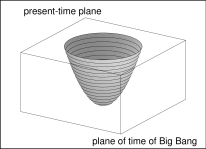
Figure 1: Schematic picture of the classical expansion of 1D Universe after Big Bang.

2 Cosmological preliminaries

There exist several imminent sources of inspiration of our present study. The oldest one is due to Ali Mostafazadeh [14]. As early as in 2001, after my seminar talk at his University he pointed out that the non-Hermitian but ${\cal PT}-$symmetric Schrödinger operators could find, via Wheeler-DeWitt equation, an important exemplification in cosmology. Although he abandoned the project a few years later (cf. his critical and sceptical summary of the outcome in his review paper [9]), the idea survived. The related necessary quantum-theoretical methods themselves are being actively developed (cf., e.g., [11] and [12]). In what follows we intend to describe briefly both their key ideas and their potential applicability in the Big Bang setting.

2.1 Big Bang in classical picture

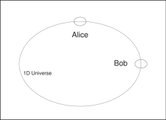
Figure 2: Alice and Bob measure their 1D distance (non-covariant idealization).

Our present methodical analysis of the Big Bang phenomenon cannot have any ambition of being realistic. In a Newtonian toy model of the evolution of an empty one-dimensional space we may visualize the history of the Universe as a circle which blows up with time (cf. Fig. 1). The hypothetical classical observers of this extremely simplified Universe are assumed co-moving with the space, detecting and confirming the Hubble’s law which controls the growth of their distance $q(t)$ with time (cf. Fig. 2 or pages 5 - 7 in monograph [2]).

After a hypothetical return to three spatial dimensions and/or to a non-isotropic spatial geometry one will have to employ, for a similar measurement, a non-planar quadruplet of classical observers (cf. Fig. 3). They may be expected to re-confirm the Hubble’s prediction of the approximate isotropy and homogeneity of the space. Thus, for our present methodical purposes we may return back to the 1D picture of Fig. 2 and consider the quantization of the single observable $q=q(t)$.

2.2 The problem of survival of singularities after quantization

One of my personal most influential discussions of the quantum Big Bang problem took place after a seminar in Paris [15] (cf. also its published version [16]) which was delivered by Wlodzimierz Piechocki from Warsaw. In his talk the speaker analyzed the quantum Friedmann-Robertson-Walker model in the setting of loop quantum gravity [17]. He explained why quantum theory, via Stone theorem [18], seems to lead to an inevitable regularization of the classical singularities. In the words supported by extensive literature [19], quantization was claimed to imply the necessity of replacement of the catastrophic dynamical Big Bang scenario by the mere smooth process called Big Bounce.

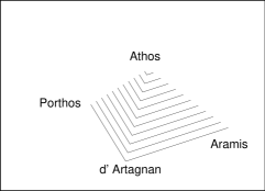
Figure 3: Four non-planar musketeers measuring their mutual distances in 3D Universe.

Besides a number of physical and thermodynamical considerations (which will not even be touched in our present text) the mathematical essence of the latter line of argumentation is comparatively easy to explain: In the absence of any symmetry (which could imply an incidental degeneracy of two eigenvalues of different symmetries) the eigenvalues of virtually any self-adjoint and parameter-dependent operator $\Lambda(\tau)$ exhibit a “repulsion” as sampled in Fig. 4.

Figure 4: Avoided crossing of eigenvalues; for Hermitian matrices the phenomenon is generic.

A rigorous mathematical explanation of the phenomenon is elementary: in similar situations the coincidence of eigenvalues at a parameter $\tau_{deg.}$ may take place if and only if this value has the properties of the so called Kato’s [20] exceptional point, $\tau_{deg.}=\tau_{(EP)}$. Alas, for self-adjoint operators the value of $\tau_{(EP)}$ is necessarily complex. Thus, whenever the parameter is time (i.e., a real variable), the evolution diagram has always the generic avoided-Big-Bang alias Big-Bounce form of Fig. 4.

3 Quantum theory preliminaries

One of the most straightforward methods of circumventing the above Big-Bang-avoiding paradox must be sought in the use of the time-dependent operators of observables $\Lambda(t)$ which possess real EP singularities. The problem becomes solvable via a parallel introduction of a nontrivial inner-product metric $\Theta=\Theta(t)$ which must also be necessarily time-dependent in general [11]. Intuitively speaking, the new degrees of freedom in $\Theta=\Theta(t)$ will suffice for an effective suppression of the repulsive tendencies of all of the eigenvalues of $\Lambda(t)$. In this manner, the currently accepted hypothesis of a mathematical necessity of the disappearance of the singularities after quantization becomes falsified.

3.1 Quantum systems in crypto-Hermitian representation

A longer version of the latter statement will form the core of our present message. We shall demonstrate the non-universality of the tunneling of Fig. 4. Our main task will be the transfer of the concept of singularities from classical gravity into the crypto-Hermitian quantum theory using the language and notation of Ref. [11].

Figure 5: The F-S-T triplet of representation spaces.

One of the quickest introductions into such a presentation of quantum theory using non-Hermitian representation of observables was provided by Scholtz et al [6]. Within the framework of nuclear physics these authors recalled the Dyson’s [5] idea that the explicit knowledge of a realistic bound-state Hamiltonian $\mathfrak{h}=\mathfrak{h}^{\dagger}$ may prove useless if its diagonalization (needed for the comparison of the theory with experiment) proves over-complicated.

The problem and its solution emerged during the study of the heaviest nuclei for which the self-adjoint realistic Hamiltonian $\mathfrak{h}$ operates in a textbook Hilbert space with the “curly-bra” vector elements $|\psi\!\!\succ\,\,\in{\cal H}^{(T)}$ (this is the notation which was introduced in Table Nr. 2 of review [11]). In the nuclear-physics literature the slow convergence of the numerical diagonalization of $\mathfrak{h}$ proved accelerated after a non-unitary preconditioning of wave functions,

$$|\psi\!\!\succ\,\,\ \ \to\ \ |\psi\rangle=\Omega^{-1}\,|\psi\!\!\succ\,\,\ \in\ {\cal H}^{(F)}\,.$$ (1)

The use of an appropriate, ad hoc “Dyson’s map” $\Omega$ and of the friendlier “interacting boson” Hilbert space ${\cal H}^{(F)}$ was recommended. The isospectrality between self-adjoint $\mathfrak{h}=\mathfrak{h}^{\dagger}$ (in ${\cal H}^{(T)}$) and its image $H=\Omega^{-1}\mathfrak{h}\Omega\neq H^{\dagger}$ (which is non-Hermitian in manifestly unphysical ${\cal H}^{(F)}$) gets explained when one changes the inner product and when one replaces the unphysical space ${\cal H}^{(F)}$ by its amended alternative ${\cal H}^{(S)}$.

The key features of the pattern are summarized in Fig. 5. In “the second” Hilbert space ${\cal H}^{(S)}$ the inner product is constructed or chosen in such a way that the isospectral (but, in “the first” Hilbert space ${\cal H}^{(F)}$, non-unitary) image $H$ of the Hamiltonian $\mathfrak{h}$ (which was, by assumption, self-adjoint in “the third” Hilbert space ${\cal H}^{(T)}$) becomes also self-adjoint. In another formulation, Hilbert spaces ${\cal H}^{(S)}$ and ${\cal H}^{(T)}$ become unitarily equivalent and, hence, they yield the undistinguishable measurable physical predictions.

3.2 Stone theorem revisited

In the language of mathematics the Stone theorem about unitary evolution [18] can be given a less common formulation even in Schrödinger picture in which the evolution is controlled by Schrödinger equation

$${\rm i}\,\partial_{t}|\psi\rangle=H\,|\psi\rangle\,$$ (2)

(here, $H$ must have real and discrete spectrum, usually also bounded from below). The unitary  evolution of ket vector $|\psi\rangle$ may still be reestablished even for $H\neq H^{\dagger}$ when using an amended inner-product metric $\Theta\neq I$. A non-equivalent Hilbert space ${\cal H}^{(S)}$ of the preceding paragraph is obtained in this manner.

The construction enables us to define a new operator adjoint $H^{\ddagger}=\Theta^{-1}H^{\dagger}\Theta$. Under certain natural conditions the same Hamiltonian $H$ may be then declared self-adjoint in ${\cal H}^{(S)}$ whenever the metric is such that $H=H^{\ddagger}$. Some of the necessary mathematical properties of the Hamiltonian-Hermitizing metric operator were thoroughly discussed in [6]. Their rigorous study may also be found in the recent edited book [21] and, in particular, in its last chapter [22].

The sense of the whole recipe is in rendering the evolution law (2) unitary in ${\cal H}^{(S)}$, i.e., fully compatible with the first principles of quantum mechanics. In other words, a unitary evolution of a quantum state in ${\cal H}^{(S)}$ may be misinterpreted as non-unitary when studied in an ill-chosen Hilbert space ${\cal H}^{(F)}$ in which the Hamiltonian is not self-adjoint, $H\neq H^{\dagger}$ [9].

3.3 Unconventional Schrödinger picture

In the the conventional Schrödinger picture (SP) the Hamiltonian $\mathfrak{h}_{(SP)}(t)$ is assumed self-adjoint in a textbook-space ${\cal H}^{(T)}$. It may be assumed to generate also the unitary evolution of the wave functions $|\psi(t)\!\!\succ\,\,$ of the Universe. Still, in the light of the preceding two paragraphs this generator may prove simplified when replaced by its isospectral, Big-Bang-passing (BBP) partner

$$H_{({BBP})}(t)=\Omega^{-1}_{({BBP})}(t)\,\mathfrak{h}_{(SP)}(t)\,\Omega_{({BBP})}(t)\,.$$ (3)

One could choose here any (i.e., in general, non-unitary and manifestly time-dependent) invertible Dyson’s operator $\Omega_{({BBP})}(t)$ which maps the initial physical Hilbert space ${\cal H}^{(T)}$ on its (in general, unphysical, auxiliary) image ${\cal H}^{(F)}$. Subsequently, one defines the so called physical metric

$$\Theta_{(BBP)}(t)=\Omega_{(BBP)}^{\dagger}\!(t)\,\,\Omega_{(BBP)}(t)\,.$$ (4)

The desired amendment of the unphysical inner product is achieved [9]. Indeed, it might look rather strange that we are now dealing with a time dependent scalar product, but an exhaustive explanation and resolution of the apparent paradox has been provided in Ref. [11]. In a way summarized in Fig. 5 above one merely returns from the auxiliary Hilbert space ${\cal H}^{(F)}$ to its ultimate physical alternative ${\cal H}^{(S)}$. By construction, the latter one is “physical”, i.e., unitarily equivalent to the initial one, ${\cal H}^{(S)}\sim{\cal H}^{(T)}$.

We are now prepared to make the next step and to return to the problem of the cosmological applicability of the whole representation pattern of Fig. 5 as summarized briefly also in subsection 3.1. First of all we have to take into consideration the manifest time-dependence of our model-dependent and geometry-representing preselected observable $Q(t)=Q_{({BBP})}(t)$. This operator is defined in both ${\cal H}^{(F)}$ and ${\cal H}^{(S)}$. Via an analogue of Eq. (3) the action of this operator may be pulled back to the initial Hilbert space ${\cal H}^{(T)}$, yielding its self-adjoint avatar

$$\mathfrak{q}_{(SP)}(t)=\Omega_{({BBP})}(t)\,Q_{({BBP})}(t)\,\Omega^{-1}_{({BBP})}(t)\,.$$ (5)

In this manner, the observability of $Q_{({BBP})}(t)$ is guaranteed if and only if

$$Q^{\dagger}_{({BBP})}(t)\Theta_{({BBP})}(t)=\Theta_{({BBP})}(t)\,Q_{({BBP})}(t)\,.$$ (6)

The latter relation may be re-read as a linear operator equation for unknown $\Theta_{({BBP})}(t)$. When solved it enables us to reconstruct (and, subsequently, factorize) the metric which we need in the applied BBP context.

In the next step of the recipe of Ref. [11] our knowledge of the time-dependent operator (3) and of the Dyson’s map $\Omega_{({BBP})}(t)$ enables us to introduce a new operator $G_{({BBP})}(t)=H_{({BBP})}(t)-{\Sigma}_{({BBP})}(t)$ where

$${\Sigma}_{({BBP})}(t)={\rm i}\Omega^{-1}_{({BBP})}(t)\left[\partial_{t}\Omega_{({BBP})}(t)\right]\,.$$ (7)

The SP evolution of wave functions in ${\cal H}^{(F)}$ and ${\cal H}^{(S)}$ will then be controlled by the pair of Schrödinger equations of Ref. [11],

$${\rm i}\partial_{t}|\Psi^{({BBP})}(t)\rangle=G_{({BBP})}(t)\,|\Psi^{({BBP})}(t)\rangle\,,\ \ \ \ \ \ |\psi^{({BBP})}(t)\rangle\in{\cal H}^{(F)}_{({BBP})}\,,$$ (8)

$${\rm i}\partial_{t}|{\Psi}^{({BBP})}(t)\rangle\!\rangle=G_{({BBP})}^{\dagger}(t)\,|{\Psi}^{({BBP})}(t)\rangle\!\rangle\,,\ \ \ \ \ \ |{\psi}^{({BBP})}(t)\rangle\!\rangle\in{\cal H}^{(F)}_{({BBP})}\,.$$ (9)

We may conclude that the time-dependence of mappings ${\Omega}_{({BBP})}(t)$ does not change the standard form of the time-evolution of wave functions too much. One only has to keep in mind that the role of the generator of the time-evolution of the wave functions is transferred from the hiddenly Hermitian “energy” operator $H_{({BBP})}(t)$ to the “generator” operator $G_{({BBP})}(t)$ which contains, due to the time-dependence of the Dyson’s map, also a Coriolis-force correction ${\Sigma}_{({BBP})}(t)$.

The second important warning concerns an innocent-looking but deceptive subtlety as discussed more thoroughly in Ref. [23]. Its essence is that the apparently independent F-space ketket solutons of the apparently independent Eq. (9) are just the S-space physical conjugates of the usual F-space kets of Eq. (8). This means that whenever one works in ${\cal H}^{(F)}$, one has to evaluate the expectation values of a generic, hiddenly Hermitian observable $A_{({BBP})}(t)$ using the F-space formula

$$\langle\!\langle\Psi^{({BBP})}(t)|A_{({BBP})}(t)|\Psi^{({BBP})}(t)\rangle\,$$ (10)

where F-kets $|{\Psi}^{({BBP})}(t)\rangle$ and $|{\Psi}^{({BBP})}(t)\rangle\!\rangle=\Theta_{(BBP)}(t)|{\Psi}^{({BBP})}(t)\rangle$ represent just an S-ket and its Hermitian S-conjugate, i.e., just the same physical quantum state.

4 Evolution in Heisenberg picture

In a Gedankenexperiment one may prepare the Universe, at some post-Big-Bang time $T>0$, in a pure state represented by a biorthogonal pair of Hilbert-space elements $|{\Psi}^{({BBP})}(T)\rangle$ and $|{\Psi}^{({BBP})}(T)\rangle\!\rangle$. In such a setting we may let the time to run backwards. Then we may solve Eqs. (8) and (9), in principle at least. This might enable us to reconstruct the past, i.e., we could specify the states of our Universe $|{\Psi}^{({BBP})}(t)\rangle$ and $|{\Psi}^{({BBP})}(t)\rangle\!\rangle$ at any $t>\tau_{(EP)}=0$.

4.1 Heisenberg equations

The consistent picture of the unfolding of the Universe after Big Bang cannot remain restricted to the description of the evolution of wave functions. The test of the predictive power of the theory can only be provided via a measurement, say, of the probabilistic distribution of data. Thus, the theoretical predictions are specified by the overlaps (10). By construction, the variations of wave functions as controlled by the generator $G_{({BBP})}(t)$ will interfere with the variations of the operator $A_{({BBP})}(t)$ itself.

In our cosmological considerations the “background of quantization” [24] characterizing the observable geometry of the empty Universe is represented by the “Alice-Bob distance” operator $Q(t)$ or, in general, by a set of such operators. They are assumed to be given as kinematical input, determining also the time-dependent Dyson’s map via Eq. (6). For all of the other, dynamical observables in ${\cal H}^{(F,S)}$, with formal definition

$$A_{({BBP})}(t)=\Omega_{({BBP})}^{-1}(t)\mathfrak{a}_{(SP)}(t){\Omega}_{({BBP})}(t)$$ (11)

a new problem emerges whenever they happen to be specified just at an “initial”/“final” time $t=T$ of the preparation/filtration of the quantum state in question. Still, the reconstruction of mean values (10) remains friendly and feasible in Heisenberg representation in which the wave functions are constant so that we must set $G(t)=0$ and $H(t)=\Sigma(t)$ (cf. Ref. [12] for more details).

Naturally, whenever we decide to turn attention to the more general non-adiabatic options with $G(t)\neq 0$, the above most convenient assumption of our input knowledge of the map ${\Omega}_{({BBP})}(t)$ may prove too strong. With the purpose of weakening it we may rewrite Eq. (7) in the Cauchy-problem form

$${\rm i}\partial_{t}\Omega_{({BBP})}(t)=\Omega_{({BBP})}(t){\Sigma}_{({BBP})}(t)\,$$ (12)

to be read as a differential-equation definition of mapping ${\Omega}_{({BBP})}(t)$ from its suitable initial value (say, at $t=T$) and from the more natural input knowledge of the Coriolis force ${\Sigma}_{({BBP})}(t)$ of Eq. (7) which strongly resembles (possibly, perturbed) Hamiltonian in Heisenberg picture.

After a return to the Heisenberg-picture assumption $H(t)=\Sigma(t)$ let us now differentiate Eq. (11) with respect to time. Once we abbreviate $\partial_{t}\mathfrak{a}_{(SP)}(t)=\mathfrak{b}(t)$ and define

$$B_{({BBP})}(t)=\Omega_{({BBP})}^{-1}(t)\mathfrak{b}(t){\Omega}_{({BBP})}(t)\,,\ \ \ \ \ H_{({BBP})}(t)=\Sigma_{({BBP})}(t)$$ (13)

this yields the first rule alias Heisenberg evolution equation

$${\rm i}\partial_{t}A_{({BBP})}(t)=A_{({BBP})}(t){H}_{({BBP})}(t)-{H}_{({BBP})}(t)A_{({BBP})}(t)+{\rm i}B_{({BBP})}(t)\,$$ (14)

and an accompanying, adjoint rule

$${\rm i}\partial_{t}A^{\dagger}_{({BBP})}(t)=A_{({BBP})}^{\dagger}(t){H}_{({BBP})}^{\dagger}(t)-{H}_{({BBP})}^{\dagger}(t)A_{({BBP})}^{\dagger}(t)+{\rm i}B_{({BBP})}^{\dagger}(t)\,.$$ (15)

Formally, both of them resemble the Heisenberg commutation relations and contain an independent-input operator (13). Naturally, the latter operator might have been given an explicit form of an $T\to F$ transfer of the anomalous time-variability of our observable whenever considered time-dependent  already in Schrödiger picture. Nevertheless, once we follow the classics [6] and once we treat any return $F\to T$ as prohibited (otherwise, the Dyson’s non-unitary mapping would lose its raison d’être), “definition” (13) is inaccessible. Due to the kinematical origin of Eqs. (14) or (15), our knowledge of operator $B_{({BBP})}(t)$ at all times must really be perceived as an independent source of input information about the dynamics.

The list of the evolution equations for a quantum system in question becomes completed. Naturally, the initial values of operators ${\Theta}_{({BBP})}(T)$ and $A_{({BBP})}(T)$ must be such that

$$A^{\dagger}_{({BBP})}(T){\Theta}_{({BBP})}(T)={\Theta}_{({BBP})}(T)A_{({BBP})}(T)\,$$ (16)

We may conclude that whenever $G(t)=0$, the construction of any concrete toy model only requires the solution of Heisenberg evolution Eqs. (14) or (15).

4.2 The limitations of the Heisenberg picture of the Universe

Before recalling any examples let us re-emphasize that the Heisenberg representation alias Heisenberg picture (HP) of the quantum systems provides one of the most straightforward forms of hypothetical transitions between classical and quantum worlds. One should immediately add that the HP approach proves extremely tedious in the vast majority of practical calculations. It replaces the dynamics described by the SP Schrödinger equation for wavefunctions by its much more complicated operator, Heisenberg-equation equivalent. At the same time, once we are given our “geometry” observable $Q(t)$ in its time-dependent Heisenberg-representation form in advance (say, in a way motivated, somehow, by the principle of correspondence), our tasks get perceivably simplified.

In the underlying theory one assumes, therefore, that the set of the admissible (and measurable) instantaneous quantized distances $q(t)=q_{n}(t)$ between the two observers of Fig. 2 are eigenvalues of an operator $Q=Q(t)$ in some physical Hilbert space ${\cal H}^{(S)}$. This space is assumed endowed with the instantaneous physical inner product which is determined, say, by a time-independent metric $\Theta\neq\Theta(t)$ [12]. In the case of a pure-state evolution, the integer subscript $n=1,2,\ldots,N$ with $N\leq\infty$ may be kept fixed via a preparation or measurement over the system at a time $t=T$.

Our quantum description of the Universe shortly after Big Bang will be based, as already indicated above, on a non-Dirac, BBP amendment of the Hilbert-space metric, on its factorization (4) and on the use of preconditioning of the “clumsy” physical wave function $|\psi(t)\!\!\succ\,\,\in{\cal H}^{(T)}$ of the Universe,

$$|\psi(t)\!\!\succ\,\,=\Omega_{(BBP)}(t)\,|\psi(t)\rangle=\left[\Omega_{(BBP)}^{\dagger}(t)\right]^{-1}|\psi(t)\rangle\!\rangle\,.$$ (17)

(cf. Eq. (1) below, and note also the unfortunate typo in equation Nr. (7) of Ref. [12] where the exponent $(^{-1})$ is missing).

As long as the mapping $\Omega$ is allowed time-dependent, the standard Schrödinger equation which determined the evolution of a pure state $|\psi(t)\!\!\succ\,\,$ in space ${\cal H}^{(T)}$ in Schrödinger picture cannot be replaced by Eq. (2) anymore. Indeed, one must leave the standard Schrödinger picture as well as its non-Hermitian stationary amendment and implementations as described in Refs. [6, 8, 9].

Secondly, without additional assumptions one cannot employ the non-Hermitian Heisenberg picture, either. The reason is that in this framework (in which the observables are allowed to vary with time) the Hilbert space metric must still be kept constant [12]. Thus, our theoretical quantum description of the evolution of the Universe in Heisenberg picture must be accompanied by the adiabaticity assumption $\partial_{t}\Theta(t)=$ small.

5 What could have happened before Big Bang?

The applicability of the above-summarized crypto-Hermitian version of Heisenberg picture of Ref. [12] may be now sampled by any above-mentioned schematic toy model of the Universe in adiabatic approximation. Operator $Q(t)$ (defined as acting in a preselected Hilbert space ${\cal H}^{(F)}$) is assumed given (or guessed, say, on the background of correspondence principle) in advance, as a tentative input information about dynamics.

In addition, our schematic Universe living near Big Bang may be also endowed with an additional pair of observables $A$ and $B$, with their mutual relation clarified by the pair of Eqs. (11) and (13). In principle, in the light of Eq. (14) the former operator may be specified just at the initial time $t=T$. In this sense the models with the necessity of specification of $B(t)\neq 0$ at all times may be considered anomalous (cf. also the related discussion in [12]).

Naturally, even if we assume that $B(t)=0$, the solution of Heisenberg Eq. (14) need not be easy. For this reason, we shall now display the results of a quantitative analysis of a few most elementary models. We shall employ the following simplifying assumptions: (1) In the spirit of Fig. 2, only the quantized distance between Alice and Bob (i.e., just a single geometry-representing and adiabatically variable observable $Q(t)$) will be considered. (2) For the sake of simplicity, our illustrative samples of the kinematical input information (i.e., of the operators $Q(t)$) will only be considered in a finite-dimensional, $N$ by $N$ matrix form, $Q(t)=Q^{(N)}(t)$.

Figure 6: Real eigenvalues of the toy-model geometry (18) in the both-sided vicinity of its Big Bang singularity at $t=0$.

5.1 No tunneling and no observable space before Big Bang

For illustration purposes let us first recall the $N$ by $N$ real matrix model of Refs. [25] with

$$Q^{(N)}(t)=Q_{0}^{(N)}+\sqrt{1-t}\times Q_{1}^{(N)}$$ (18)

which is composed of a diagonal matrix $Q_{0}^{(N)}$ with equidistant elements

$$\left[Q_{0}^{(N)}\right]_{nn}=\{-N+1,-N+3,\ldots,N-1\}$$ (19)

and of an antisymmetric time-dependent “perturbation” with a tridiagonal-matrix coefficient $Q_{1}^{(N)}$ with zero diagonal and non-vanishing elements $\left[Q_{0}^{(N)}\right]_{n+1,n}=-\left[Q_{0}^{(N)}\right]_{n,n+1}=$

$$=\{\sqrt{1\cdot(N-1)},\sqrt{2\cdot(N-2)},\sqrt{3\cdot(N-3)},\ldots,\sqrt{(N-1)\cdot 1},\}\,.$$ (20)

In Refs. [25] the choice of this model was dictated by its property of having real and equidistant spectrum at all of the non-negative times $t>0$. Another remarkable feature of this model is that while matrix (18) is real and manifestly non-Hermitian at all times $t\in(-\infty,1)$, it becomes diagonal at $t=1$ and complex and Hermitian at all the remaining times $t\in(1,\infty)$.

At $N=10$ the spectrum of such a toy model is sampled in Fig. 6. Obviously, this example of a kinematical input connects, smoothly, the complete Big-Bang-type degeneracy of the eigenvalues at $t=0$ with their unfolding at $t>0$ which passes also through the “unperturbed”, diagonal-matrix special case at $t=1$. Needless to emphasize that in this model the spectrum is all complex and, hence, the space of the Universe remains completely unobservable alias non-existent before Big Bang.

5.2 Cyclic cosmology

Not quite expectedly the spectrum gets entirely different after an apparently minor change of the time-dependence in

$$Q^{(N)}(t)=Q_{0}^{(N)}+\sqrt{1-t^{2}}\times Q_{1}^{(N)}$$ (21)

Using $N=8$ the resulting spectrum is displayed in Fig. 7. We see that in the new model the “geometry of the world” was the same before Big Bang so that model (21) may be perceived as reflecting a kinematics of a kind of cyclic cosmology as preferred in Hinduism or, more recently, by Roger Penrose [26].

Figure 7: Real eigenvalues of the toy-model geometry (21) in the both-sided vicinity of its Big Bang singularity at $t=0$.

5.3 Darwinistic, evolutionary cosmology

In the THS representation of the 1D Universe the “geometry” or “kinematical” operator $Q(t)$ may be assumed, in general,

• non-Hermitian (otherwise, we would lose the dynamical degrees of freedom carried by the generic metric $\Theta$ and needed and essential near the Big Bang instant),

• simple (i.e., typically, tridiagonal as above – otherwise, there would be hardly any point in our leaving the much simpler Schrödinger picture).

In the latter sense, our third class of toy models may be taken from Refs. [27] and  [28] and sampled by the following $N=8$ distance operator

$$Q(t)=\left[\begin{array}[]{cccccccc}0&1-t&0&0&0&0&0&0\\ \vskip 6.0pt plus 2.0pt minus 2.0pt\cr t&0&1-t&0&0&0&0&0\\ \vskip 6.0pt plus 2.0pt minus 2.0pt\cr 0&t&0&1-\left|t\right|&0&0&0&0\\ \vskip 6.0pt plus 2.0pt minus 2.0pt\cr 0&0&\left|t\right|&0&1-\left|t\right|&0&0&0\\ \vskip 6.0pt plus 2.0pt minus 2.0pt\cr 0&0&0&\left|t\right|&0&1-\left|t\right|&0&0\\ \vskip 6.0pt plus 2.0pt minus 2.0pt\cr 0&0&0&0&\left|t\right|&0&1-t&0\\ \vskip 6.0pt plus 2.0pt minus 2.0pt\cr 0&0&0&0&0&t&0&1-t\\ \vskip 6.0pt plus 2.0pt minus 2.0pt\cr 0&0&0&0&0&0&t&0\end{array}\right]\,$$ (22)

The piecewise linear time-dependence of this operator leads to the quantum phase transition between the Big Crunch collapse of the spatial grid in previous Eon and the Big Bang start of the spatial expansion of the present Eon. In the vicinity of the singularity at $t=0$ we may characterize such a quantum cosmological toy model by the following flowchart,

$$\\ \begin{array}[]{c}\ \ \ \ \ \ \ \ \ \ \ \ \ \begin{array}[]{|c|}\hline\cr{\rm{\bf working}\ space\ }{\cal H}^{(F)}\\ {\rm the\ observable\ of\ {\bf geometry}\ }Q(t)\\ {\rm defined\ at\ all\ real\ times}\\ {\rm{\bf non-diagonalizable}\ at\ }t_{(EP)}=0\\ \hline\cr\end{array}\\ \\ \stackrel{{\scriptstyle{\bf previous\ Eon,}}}{{t<0}}\ \swarrow\ \ \ \ \ \ \ \ \ \ \ \ \ \ \ \ \ \ \ \searrow\ \ \ \stackrel{{\scriptstyle{\bf our\ Eon,}}}{{t>0}}\\ \\ \ \ \ \ \ \ \ \ \begin{array}[]{|c|}\hline\cr{\rm{\bf underdeveloped\ }standard\ space\ }{\cal H}^{({S^{\prime}})}\\ {\rm{\bf ghosts\ }to\ be\ projected\ out}\\ {\rm(some\ eigenvalues\ {\bf not\ yet}\ observable)}\\ \hline\cr\end{array}\ \ \ \ \ \ \ \ \ \begin{array}[]{|c|}\hline\cr{\rm{\bf our\ }Hilbert\ space}\ {\cal H}^{(S)}\\ {\rm observable\ }{Q}={Q}^{\ddagger}=\Theta_{S}^{-1}Q^{\dagger}\Theta_{S}\\ {\rm(all\ eigenvalues\ {\bf real})}\\ \hline\cr\end{array}\\ \\ \ \swarrow\!\!\!\ \ \ \ \ \ \stackrel{{\scriptstyle{\bf auxiliary\ maps\ to\ Schroedinger\ picture}}}{{}}\ \ \ \ \searrow\!\!\!\\ \\ \begin{array}[]{|c|}\hline\cr{\rm{}third\ space}\ {\cal H}^{(T^{\prime})}\\ {\rm of\ the\ {\bf extinct\ }Universe}\\ \hline\cr\end{array}\ \ \ \ \ \ \ \ \ \ \ \ \ \ \ \ \ \ \ \ \ \ \ \ \ \begin{array}[]{|c|}\hline\cr{\rm{}third\ space}\ {\cal H}^{(T)}\\ {\rm{\bf contemporary\ }Universe}\\ \hline\cr\end{array}\,.\\ \end{array}\\ \\$$

The evolutionary-cosmology idea of the quantum Crunch-Bang transition itself (discussed more thoroughly in Ref. [28] and illustrated also by Fig. 8) may be perceived as one of the serendipitous conceptual innovations provided by the present Heisenberg-picture background-independent [24] quantization of our schematic Universes.

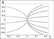
Figure 8: Real eigenvalues of the toy-model geometry (22) in the both-sided vicinity of the Crunch-Bang singularity at $t=0$.

6 Outlook

The results of the analysis of the solvable models of preceding section offer a nice illustration of several merits of the THS approach to the building of Big-Bang-exhibiting quantum systems.

• the Big Bang value of time $t^{(BB)}=0$ is a point of degeneracy of all of the eigenvalues, $q_{n}(0)=0$ at all $n=1,2,\ldots,N$;

• at $t=t^{(BB)}=0$ all of our toy models acquire the complete, $N$ by $N$ Jordan-block structure so that the Big Bang time coincides with the point of confluence of all of the Kato’s exceptional points;

• after Big Bang, i.e., at $t>t^{(BB)}=0$ the spectra of possible (and growing) quantum distances between Alice and Bob are all real and, hence, observable, in our specific toy models at least;

• in the light of Fig. 8 our models describe also the times before Big Bang, $t<t^{(BB)}=0$. In this sense the pass of our systems through the Big-Bang singularity is “causal”, described by a “universal” operator $Q(t)$;

• before Big Bang (i.e., before the Big Crunch of the Penrose’s [26] “previous Eon”) the menu of the real distances $q_{n}(t)$ is replaced by an empty set (in Fig. 6), survives unchanged (in Fig. 7) or gets reduced to a proper subset (cf. Fig. 8);

• in the most interesting latter case the “missing”, complex eigenvalues are tractable as “not yet observable”. One could speak about various “evolutionary” forms of cosmology in this setting.

Appendix. Auxiliary spaces and ${\cal PT}$ symmetries

A few years after the publication of review [6], a series of rediscoveries and an enormous growth of popularity of the pattern followed the publication of pioneering letter [29] in which Bender with his student inverted the flowchart. They choose a nice illustrative example to show that the manifestly non-Hermitian $F-$space Hamiltonian $H$ with real spectrum may be interpreted as a hypothetical input information about the dynamics (cf. also review [8] for more details).

Graphically, the flowchart of ${\cal PT}-$symmetric quantum theory is schematically depicted in Fig. 9. For completeness let us add that the Bender’s and Boettcher’s construction was based on the assumption of ${\cal PT}$ symmetry $H{\cal PT}={\cal PT}H$ of their dynamical-input Hamiltonians where the most common phenomenological parity ${\cal P}$ and time reversal ${\cal T}$ entered the game. Mostafazadeh (cf. his review [9]) emphasized that their theory may be generalized while working with more general ${\cal T}$s (typically, any antilinear operator) and ${\cal P}$s (basically, any indefinite, invertible operator).

Several mathematical amendments of the theory were developed in the related literature, with the main purpose of making the constructions feasible. Let us only mention here that the useful heuristic role of operator ${\cal P}$ was successfully transferred to the Krein-space metrics $\eta$ (cf. [30] for a comprehensive review). In comment [31] we explained that in principle, the role of ${\cal P}$ could even be transferred to some positive-definite, simplified and redundant auxiliary-Hilbert-space metrics $\tilde{\cal P}=\Theta_{A}\neq\Theta_{S}$. Such a recipe proved encouragingly efficient [32]. Its flowchart may be summarized in the following diagram

$$\\ \begin{array}[]{c}\ \ \ \begin{array}[]{|c|}\hline\cr\framebox{\rm input:}\\ {\bf space}\ {\cal H}^{(F)}\ {\rm is}\ {\bf friendly}\\ {\bf metric\ }\Theta^{(Dirac)}=I\ {\rm is}\ {\bf false}\\ {\rm observable\ }{{Q}(t)}\neq{{Q}}^{\dagger}(t)\ {\rm is}\ given\\ \hline\cr\end{array}\\ \\ \ \ \ \ \stackrel{{\scriptstyle{\bf\ preliminary\ Dyson\ map\ }}}{{\ }}\swarrow\ \ \ \ \ \ \ \ \ \ \ \ \ \ \ \ \ \ \ \ \ \ \ \searrow\ \ \ \stackrel{{\scriptstyle{\bf\ correct\ Dyson\ map\ }}}{{\ }}\\ \\ \ \ \ \ \begin{array}[]{|c|}\hline\cr\framebox{\rm reality\ proof:}\\ {\rm{\bf artificial\ }space\ }{\cal H}^{(A)}\\ {\rm{\bf auxiliary\ }}\Theta_{A}=\Omega_{A}^{\dagger}\Omega_{A}\\ {Q}^{\sharp}=\Theta_{A}^{-1}Q^{\dagger}\Theta_{A}={Q}\\ \hline\cr\end{array}\ \ \ \ \ \ \ \ \stackrel{{\scriptstyle{\bf not\ related\ to}}}{{}}\ \ \ \ \ \ \ \begin{array}[]{|c|}\hline\cr\framebox{\rm output:}\\ {\rm{\bf standard\ }space}\ {\cal H}^{(S)}\\ {\bf correct\ }\Theta_{S}=\Omega_{S}^{\dagger}\Omega_{S}\\ {Q}^{\ddagger}=\Theta_{S}^{-1}Q^{\dagger}\Theta_{S}={Q}\\ \hline\cr\end{array}\\ \\ \ \swarrow\!\!\!\nearrow\ \ \ \ \ \ \ \ \ \ \ \ \ \ \ \ \ \ \ \stackrel{{\scriptstyle{\bf unitary\ equivalences}}}{{}}\ \ \ \ \ \ \ \ \ \ \ \ \ \ \ \ \searrow\!\!\!\nwarrow\\ \\ \ \begin{array}[]{|c|}\hline\cr{\rm{\bf byproduct\ }}\ {\cal H}_{(math.)}\\ {\mathfrak{q}}_{(math.)}=\Omega_{A}Q\Omega_{A}^{-1}={\mathfrak{q}}_{(math.)}^{\dagger}\\ {\rm(redundant)}\\ \hline\cr\end{array}\ \ \ \stackrel{{\scriptstyle{\bf not\ related\ to}}}{{}}\ \ \begin{array}[]{|c|}\hline\cr{\rm{\bf textbook\ }space}\ {\cal H}^{(T)}_{(phys.)}\\ {\mathfrak{q}}_{(phys.)}={\mathfrak{q}}^{\dagger}_{(phys.)}={\rm\ realistic}\\ {\rm(inaccessible)}\\ \hline\cr\end{array}\\ \end{array}\\ \\$$

Besides the right-side flow of mapping we see here the auxiliary, unphysical left-side flow where, typically, the non-Dirac metric $\Theta_{A}$ need not carry any physical contents. In some models such an auxiliary metric proved even obtainable in a trivial diagonal-matrix form [28].

Figure 9: THS interpretation of ${\cal PT}-$ symmetric Hamiltonians $H$.

References

- [1] C. L. Bennett, D. Larson et al., Astrophys. J. Suppl. Ser. 208 (2013) UNSP 20.
- [2] V. Mukhanov, Physical Foundations of Cosmology (CUP, Cambridge, 2005).
- [3] C. Rovelli, Quantum Gravity (CUP, Cambridge, 2004).
- [4] M. Znojil, ”Non-self-adjoint operators in quantum physics: ideas, people, and trends”, in Ref. [21], pp. 7 - 58.
- [5] F. J. Dyson, Phys. Rev. 102 (1956) 1217.
- [6] F. G. Scholtz, H. B. Geyer and F. J. W. Hahne, Ann. Phys. (NY) 213 (1992) 74.
- [7] C. M. Bender and S. Boettcher, Phys. Rev. Lett. 80 (1998) 5243; C. M. Bender, D. C. Brody and H. F. Jones, Phys. Rev. Lett. 89 (2002) 270401 and Phys. Rev. Lett. 92 (2004) 119902 (erratum).
- [8] C. M. Bender, Reports on Progress in Physics 70 (2007) 947.
- [9] A. Mostafazadeh, Int. J. Geom. Meth. Mod. Phys. 7 (2010) 1191.
- [10] A. V. Smilga, J. Phys. A: Math. Theor. 41 (2008) 244026.
- [11] M. Znojil, SIGMA 5 (2009) 001 (arXiv overlay: 0901.0700).
- [12] M. Znojil, Phys. Lett. A 379 (2015) 2013.
- [13] M. Znojil, Phys. Rev. D 78 (2008) 085003.
- [14] A. Mostafazadeh, private communication.
- [15] W. Piechocki, APC seminar “Solving the general cosmological singularity problem”, Paris, November 15, 2012.
- [16] P. Malkiewicz and W. Piechocki, Class. Quant. Gravity 27 (2010) 225018.
- [17] A. Ashtekar, A. Corichi and P. Singh, Phys. Rev. D 77 (2008) 024046.
- [18] M. H. Stone, Ann. Math. 33 (1932) 643.
- [19] A. Ashtekar, T. Pawlowski and P. Singh, Phys. Rev. D 74 (2006) 084003.
- [20] T. Kato, Perturbation Theory for Linear Operators (Springer-Verlag, Berlin, 1966).
- [21] F. Bagarello, J.-P. Gazeau, F. H. Szafraniec and M. Znojil (Ed.), Non-Selfadjoint Operators in Quantum Physics: Mathematical Aspects (John Wiley & Sons, Hoboken, 2015).
- [22] J.-P. Antoine and C. Trapani, ”Metric operators, generalized Hermiticity and lattices of Hilbert spaces”, in Ref. [21], pp. 345 - 402.
- [23] M. Znojil, SIGMA 4 (2008) 001 (arXiv overlay: 0710.4432v3).
- [24] T. Thiemann, Modern Canonical Quantum General Relativity (CUP, Cambridge, 2007).
- [25] M. Znojil, J. Phys. A: Math. Theor. 40 (2007) 4863; M. Znojil, J. Phys. A: Math. Theor. 40 (2007) 13131.
- [26] R. Penrose, Found. Phys. 44 (2014) 873.
- [27] M. Znojil and J.-D. Wu, Int. J. Theor. Phys. 52 (2013) 2152.
- [28] D. I. Borisov, F. Ruzicka and M. Znojil, Int. J. Theor. Phys. 54 (2015) 4293.
- [29] C. M. Bender and S. Boettcher, Phys. Rev. Lett. 80 (1998) 5243.
- [30] S. Albeverio and S Kuzhel, ”PT-symmetric operators in quantum mechanics: Krein spaces methods”, in Ref. [21], pp. 293 - 344.
- [31] M. Znojil and H. B. Geyer, Fort. d. Physik - Prog. Phys. 61 (2013) 111.
- [32] M. Znojil, Ann. Phys. (NY) 361 (2015) 226.