The dust properties and physical conditions of the interstellar medium in the LMC massive star forming complex N11

Abstract

We combine Spitzer and Herschel data of the star-forming region N11 in the Large Magellanic Cloud to produce detailed maps of the dust properties in the complex and study their variations with the ISM conditions. We also compare APEX/LABOCA 870$\mu$m observations with our model predictions in order to decompose the 870 $\mu$m emission into dust and non-dust (free-free emission and CO(3-2) line) contributions. We find that in N11, the 870 $\mu$m can be fully accounted for by these 3 components. The dust surface density map of N11 is combined with H i and CO observations to study local variations in the gas-to-dust mass ratios. Our analysis leads to values lower than those expected from the LMC low-metallicity as well as to a decrease of the gas-to-dust mass ratio with the dust surface density. We explore potential hypotheses that could explain the low ‘observed’ gas-to-dust mass ratios (variations in the X_CO factor, presence of CO-dark gas or of optically thick H i or variations in the dust abundance in the dense regions). We finally decompose the local SEDs using a Principal Component Analysis (i.e. with no a priori assumption on the dust composition in the complex). Our results lead to a promising decomposition of the local SEDs in various dust components (hot, warm, cold) coherent with that expected for the region. Further analysis on a larger sample of galaxies will follow in order to understand how unique this decomposition is or how it evolves from one environment to another.

1 Introduction

Measuring the different gas and dust reservoirs and their dependence on the physical conditions in the interstellar medium (ISM) is fundamental to further our understanding of star formation in galaxies and understand their chemical evolution. However, the various methods used to trace these reservoirs have a number of fundamental flaws. For instance, CO observations are often used to indirectly trace the molecular hydrogen H₂ in galaxies. Departures from the well-constrained Galactic conversion factor between the CO line intensity and the H₂ mass - the so-called X_CO factor - are expected on local (region to region) or global (galaxy to galaxy) scales. However, these variations are still poorly understood. Dust emission in the IR-to-submillimeter regime is often used as a complementary tracer of the gas reservoirs. This technique, however, also requires assumptions on both the dust composition and the gas-to-dust mass ratio (GDR). Both quantities also vary from one environment to another.

All these effects are even less constrained at lower metallicities. In a dust-poor environment for instance, UV photons penetrate more easily in the ISM, creating large reservoirs of gas where H₂ is efficiently self-shielded but CO is photo-dissociated, thus not properly tracing H₂. The conversion factor X_CO thus strongly depends on the dust content and the ISM morphology (we refer to Bolatto et al., 2013, for a review on X_CO). In these metal-poor environments, dust appears as a less biased tracer of the gaseous phase. However, metallicity also affects the dust properties, whether we are talking about the size distribution of the dust grains (Galliano et al., 2005) or their composition. Submillimeter (submm) observations with the Herschel Space Observatory or from the ground have in particular helped us characterize the variations of the cold dust properties (dust emissivity, submm excess) with the physical conditions of the ISM (Rémy-Ruyer et al., 2014, 2015).

Further studies targeting a wide range of physical conditions, with a particular focus on lower metallicity environments, are necessary to understand the dust and the gas reservoirs and study the influence of standard assumptions on their apparent relations. This paper is part of a series to study the ISM components in the nearby Large Magellanic Cloud (LMC) at small spatial scales. The LMC is a prime extragalactic laboratory to perform a detailed study of low metallicity ISM (Z_LMC = 1/2 $Z_{\odot}$; Dufour et al., 1982). Its proximity (50 kpc; Schaefer, 2008) and its almost face-on orientation (23-37^∘; Subramanian & Subramaniam, 2012) enable us to study its star forming complexes at a resolution of 10 pc (the best resolution currently available for external galaxies). This analysis aims to constrain the dust and gas properties along a large number of sight-lines toward N11, the second brightest H ii region in the LMC. This paper has three main goals. Our first goal is to model the local infrared (IR) to submm dust Spectral Energy Distributions (SED) across the N11 complex in order to provide maps of the dust parameters (excitation, dust column density) and study their dependence on the ISM physical conditions. The second goal is to relate the dust reservoir to the atomic and molecular gas reservoirs in order to study the local variations in GDR and understand their origin. The methodologies we discuss will enable us to gauge the effects of the various assumptions on the derived GDR observed. The last goal is to explore a Principal Component Analysis (PCA) of the local SEDs as an alternative and possibly promising method to investigate the “resolved” dust populations in galaxies with no a priori assumption on the dust composition.

We describe the N11 star-forming complex, the Spitzer, Herschel and LABOCA observations and the correlations between these different bands in $\S$2. We present the SED modeling technique we apply on resolved scales in $\S$3 and describe the dust properties we obtain (dust temperatures, mean stellar radiation field intensities) in $\S$4. We also analyze the origin of the 870 $\mu$m emission in this section. We compare the dust and gas reservoirs and discuss the implications of the low gas-to-dust we observe in $\S$5. We finally provide the results of the Principal Component Analysis we perform on the N11 local SEDs in $\S$6.

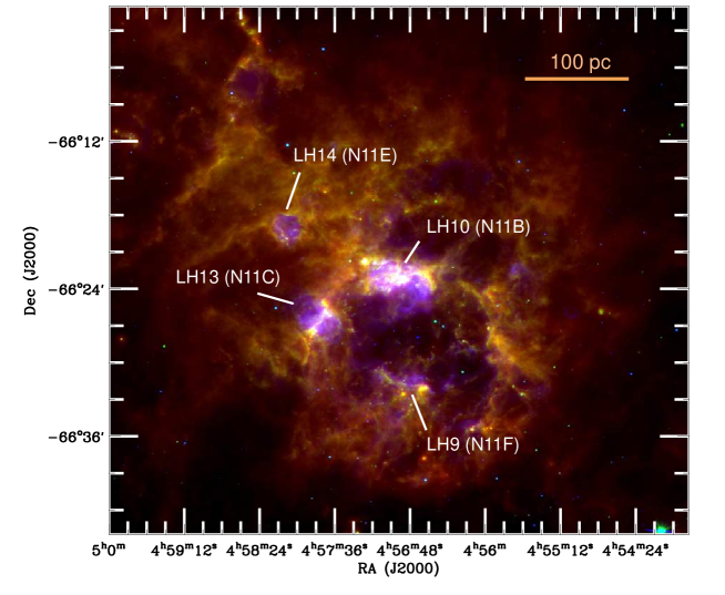
Figure 1: Color-composition of N11 with H$\alpha$ in blue, IRAC 8 $\mu$m in green and SPIRE 250 $\mu$m in red. The 4 main OB associations are indicated (from north to south: LH14 in the nebula N11E, LH10 in N11B, LH13 in N11C and LH9 at the center of the N11 cavity in the nebula N11F). The H$\alpha$ image was taken as part of the Magellanic Cloud Emission Line Survey (MCELS; Smith & MCELS Team, 1998). For all the maps in this paper, north is up, east is left and coordinates (RA, Dec) are given in equinox J2000.

2 Observations

2.1 The N11 complex

On the north-west edge of the galaxy, N11 is the second brightest H ii region in the LMC (after 30 Doradus; Kennicutt & Hodge, 1986). It exhibits several prominent secondary H ii regions along its periphery as well as dense filamentary ISM structures, as traced by the prominent dust and CO emission. It is characterized by an evacuated central cavity with an inner diameter of 170 pc. Four star clusters are the main sources of the ionization in the complex (see Lucke & Hodge (1970) or Bica et al. (2008) for studies of the stellar associations in the whole LMC). These clusters are indicated in Fig. 1. The rich OB association LH9 is located at the center of the cavity. The age of this cluster was estimated to be $\sim$7 Myr (Mokiem et al., 2007). The star cluster LH10 ($\sim$3 Myr old, Mokiem et al., 2007), is located in the north-east region of the cavity and is embedded in the N11B nebula. The OB association LH13 and its corresponding nebula (N11C) are located on the eastern edge of the super-bubble. The main exciting source of N11C is the compact star cluster Sk-66^∘41 ($<$5 Myr old; Heydari-Malayeri et al., 2000). Finally, the OB association LH14 (in N11E) is located in the northeastern filament. Its main exciting source is the Sk-66^∘43 star cluster. The region also harbors a few massive stars (see Heydari-Malayeri et al. (1987) for a detail on its stellar content). The cluster ages and the initial mass functions of the OB associations suggest a sequential star formation in N11, with a star formation in the peripheral molecular clouds triggered by the central LH9 association (Rosado et al., 1996; Hatano et al., 2006, among others). N11 is also associated with a giant molecular complex. Israel et al. (2003) and Herrera et al. (2013) have suggested that N11 is a shell compounded of discrete CO clouds (rather than bright clouds bathing in continuous inter cloud CO emission) and estimate that more than 50 $\%$ of the CO emission resides in discrete molecular clumps.

To construct our local IR to submm SEDs in N11, we use data from the Spitzer Space Telescope (Werner et al., 2004) and the Herschel Space Observatory (Pilbratt et al., 2010). We complement the submm coverage with observations obtained on the Large APEX Bolometer Camera (LABOCA) instrument at 870$\mu$m.

2.2 Spitzer IRAC and MIPS

The LMC has been observed with Spitzer as part of the SAGE project (Meixner et al., 2006, Surveying the Agents of a Galaxy’s Evolution;) and the Spitzer IRAC (InfraRed Array Camera; Fazio et al., 2004) and MIPS (Multiband Imaging Photometer; Rieke et al., 2004) and data have been reduced by the SAGE consortium. IRAC observed at 3.6, 4.5, 5.8, and 8 $\mu$m (full width half maximum (FWHM) of its point spread function (PSF) $<$2″). The calibration errors of IRAC maps are 2$\%$ (Reach et al., 2005). MIPS observed at 24, 70 and 160 $\mu$m (PSF FWHMs of 6″, 18″ and 40″ respectively). The MIPS 160 $\mu$m map of N11 is not used in the following analysis because of its lower resolution (40″) than to PACS 160 $\mu$m but the data is used for the calibration of the Herschel/PACS 160 $\mu$m map (see $\S$2.4). The respective calibration errors in the MIPS 24 and 70 $\mu$m observations are 4 and 5$\%$ (Engelbracht et al., 2007; Gordon et al., 2007). We refer to Meixner et al. (2006) for a detailed description of the various steps of the data reduction. Additional steps have been added to the SAGE MIPS data reduction pipeline by Gordon et al. (2014) (see $\S$2.5).

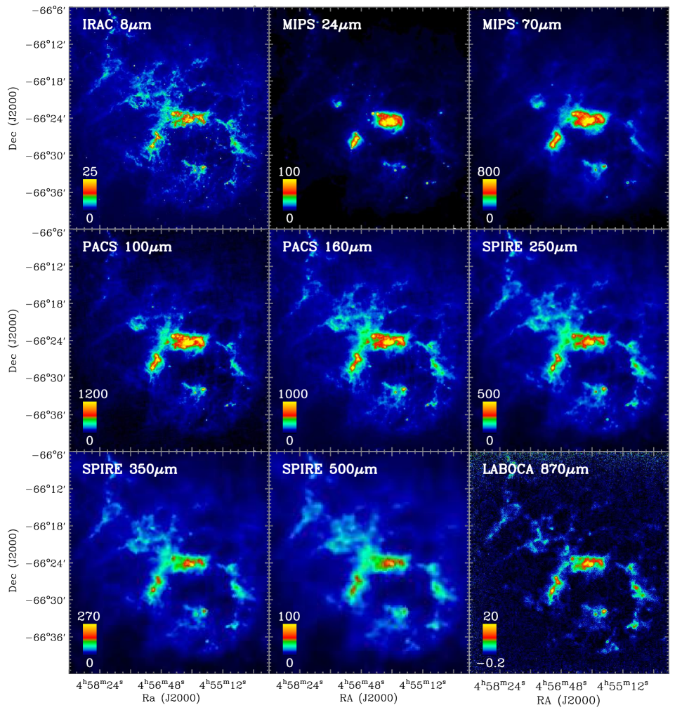
Figure 2: The IR/submm emission of the N11 star-forming complex from 8 to 870 $\mu$m (original resolution). The color bars indicate the intensity scale in MJy sr^-1. Square root scaling has been applied in order to enhance the fainter structures.

2.3 Herschel PACS and SPIRE

The LMC has been observed with Herschel as part of the successor project of SAGE, HERITAGE (HERschel Inventory of The Agents of Galaxy’s Evolution; Meixner et al., 2010, 2013). The Herschel PACS (Photodetector Array Camera and Spectrometer; Poglitsch et al., 2010) and SPIRE (Spectral and Photometric Imaging Receiver; Griffin et al., 2010) and data have been reduced by the HERITAGE consortium. The LMC was mapped at 100 and 160 $\mu$m with PACS (PSF FWHMs of $\sim$7$\aas@@fstack{\prime\prime}$7 and $\sim$12″ respectively) and 250, 350 and 500 $\mu$m with SPIRE (PSF FWHMs of 18″, 25″and 36″ respectively). The SPIRE 500 $\mu$m map possesses the lowest resolution (FWHM: 36″) of the IR-to-submm dataset. Details of the Herschel data reduction can be found in Meixner et al. (2013). We particularly refer the reader to the $\S$3.9 that describes the cross-calibration applied between the two PACS maps and the IRAS 100 $\mu$m (Schwering, 1989) and the MIPS 160 $\mu$m maps (Meixner et al., 2006) in order to correct for the drifting baseline of the PACS bolometers. The PACS instrument has an absolute uncertainty of $\sim$5$\%$ (the accuracy is mostly limited by the uncertainty of the celestial standard models used to derive the absolute calibration; Balog et al., 2014) to which we linearly add an additional 5$\%$ to account for uncertainties in the total beam area. The SPIRE instrument has an absolute calibration uncertainty of 5$\%$ to which we linearly add an additional 4$\%$ to account for the uncertainty in the total beam area (Griffin et al., 2013). Additional steps have been added to the HERITAGE PACS and SPIRE data reduction pipelines by Gordon et al. (2014) (see $\S$2.5).

Table 1: Spearman rank correlation coefficients between the IR/submm luminosities from 8 to 870 $\mu$m (log $\nu$L_ν).

Band	8 $\mu$m	24 $\mu$m	70 $\mu$m	100 $\mu$m	160 $\mu$m	250 $\mu$m	350 $\mu$m	500 $\mu$m
24$\mu$m	0.85
70$\mu$m	0.86	0.93
100$\mu$m	0.93	0.93	0.96
160$\mu$m	0.96	0.87	0.90	0.96
250$\mu$m	0.97	0.85	0.86	0.94	0.97
350$\mu$m	0.95	0.83	0.82	0.91	0.96	1.00
500$\mu$m	0.94	0.81	0.80	0.89	0.94	0.99	1.00
870$\mu$m	0.73	0.68	0.63	0.69	0.73	0.77	0.78	0.79

2.4 LABOCA observations and data reduction

LABOCA is a submm bolometer array installed on the APEX (Atacama Pathfinder EXperiment) telescope in North Chile. Its under-sampled field of view is 11$\aas@@fstack{\prime}$4 and its PSF FWHM is 19$\aas@@fstack{\prime\prime}$5, thus a resolution equivalent to that of the SPIRE 250 $\mu$m instrument onboard Herschel. N11 was observed at 870 $\mu$m with LABOCA in December 2008 and April, July and September 2009 (Program ID: O-081.F-9329A-2008 - PI: Hony). A raster of spiral patterns was used to obtain a regularly sampled map. Data are reduced with BoA (BOlometer Array Analysis Software). Every scan is reduced individually. They are first calibrated using the observations of planets (Mars, Uranus, Venus, Jupiter and Neptune) as well as secondary calibrators (PMNJ0450-8100, PMNJ0210-5101, PMNJ0303-6211, PKS0537-441, PKS0506-61, CW-Leo, Carina, V883-ORI, N2071IR and VY-CMa). Zenith opacities are obtained using a linear combination of the opacity determined via skydips and that computed from the precipitable water vapor. We also remove dead or noisy channels, subtract the correlated noise induced by the coupling of amplifier boxes and cables of the detectors. Stationary points and data taken at fast scanning velocity or above an acceleration threshold are removed from the time-ordered data stream. Our reduction procedure then includes steps of median noise removal, baseline correction (order 1) and despiking. The reduced scans are then combined into a final map in BoA. As noticed in Galametz et al. (2013), the steps of median noise removal or baseline correction are responsible for the over-subtraction of faint extended emission around the bright structures. In order to recover (most of) this extended emission we apply and additional iterative process to the data treatment. We use the reduced map as a “source model” and isolate pixels above a given signal-to-noise. This source model is masked or subtracted from the time-ordered data stream before the median noise removal, baseline correction or despiking steps of the following iteration, then added back in. We repeat the process until the process converges. Final rms and signal-to-noise maps are then generated. The average rms across the field is $\sim$8.4 mJy beam^-1. Figure 2 shows the final LABOCA map. We can see that our iterative data reduction helps us to significantly recover and resolve low surface brightnesses around the main structure of the complex.

2.5 Preparation of the IR/submm data for the analysis

We use the SAGE and HERITAGE MIPS, PACS and SPIRE maps of the LMC reprocessed by Gordon et al. (2014) in the following analysis. They include an additional step of foreground subtraction in order to remove the contamination by Milky Way (MW) cirrus dust. The morphology of the MW dust contamination has been predicted using the integrated velocity H i gas map along the LMC line of sight and using the Desert et al. (1990) model to convert the H i column density into expected contamination in the PACS and SPIRE bands. The image background is also estimated using a surface polynomial interpolation of the external regions of the LMC and subtracted from each image. All the maps are convolved to the resolution of SPIRE 500 $\mu$m (FWHM: 36″) using the convolution kernels developed by Aniano et al. (2011). We refer to Gordon et al. (2014) for further details on these additional steps. We convolve the IRAC and LABOCA maps using the same convolution kernel library. For these maps, we estimate the background from each image by masking the emission linked with the complex, fitting the distribution of the remaining pixels with a Gaussian and using the peak value as a background estimate. Pixels of the final maps are 14″, which corresponds to 3.4pc at the distance of the LMC.

2.6 Qualitative description of the dust emission

Figure 2 first shows the IRAC 8 $\mu$m, MIPS 24 and 70 $\mu$m, the two PACS and three SPIRE maps at their respective original resolutions. The emission in the 8 $\mu$m band observed with the IRAC instrument is primarily coming from polycyclic aromatic hydrocarbons (PAH). PAHs are large organic molecules thought to be responsible of the broad emission features often detected in the near- to mid-IR bands. They are present everywhere across the complex. The 24 $\mu$m emission is a tracer of the hottest dust populations. Primarily associated with H ii regions, it is often used (by itself or combined with other tracers) as a calibrator of the star formation rate (SFR, Calzetti, 2007) in nearby objects. We observe that the MIPS 24 $\mu$m emission is more compact than that at longer wavelengths and peaks in the H ii regions of the N11 complex. The MIPS 70 $\mu$m band is essential to properly constrain the Wien side of the FIR SEDs and traces the warm dust in the complex. Part of the 70 $\mu$m emission could also be associated with a very small grain (VSG) population. Studies at 70 $\mu$m in the LMC have indeed revealed a population of VSG ($<$10nm; so larger than PAH molecules) probably produced through erosion processes of larger grains in the diffuse medium (Lisenfeld et al., 2001; Bernard et al., 2008). Erosion processes in magellanic-type galaxies has also been discussed in Galliano et al. (2003, 2005). The emission above 100 $\mu$m is mostly produced by a mixture of equilibrium big ($>$25nm) silicate and carbonaceous grains (see Draine & Li, 2001, among others). The PACS 100 and 160 $\mu$m observations are associated with the cool to warm dust reservoirs (20-40K) in the complex: the observations enable us to sample the peak of the dust thermal emission across the field. Residual stripping can be observed in these maps. The SPIRE 250 to 500 $\mu$m observations are associated with the coldest dust emission ($<$20K): they will help us constrain the local dust masses as well as investigate potential emissivity variations of the dust grains in N11.

Using the Spitzer, Herschel and LABOCA maps convolved to a common 36″ resolution ($\S$2.4), we calculate the Spearman rank correlation coefficients between the various bands (log scale) for ISM elements that fulfill a 2-$\sigma$ detection criterion in the Herschel bands. Those coefficients are tabulated in Table 1 and highlight the high correlation between the various wavelengths. Correlation coefficients between the 8 $\mu$m map and bands longward of 8 $\mu$m are similar when the 8 $\mu$m map is first corrected from stellar continuum (same to the second decimal place). The 8 $\mu$m is more strongly correlated with the emission of cold dust traced by the SPIRE bands than with the tracers of hot and warm dust. This could be due to the fact that PAHs (that the 8 $\mu$m emission mostly traces) are emitted at the surface of the molecular clouds where the shielded dust remains cold. The surface of a cloud (PAH emission) and its interior (cold dust emission) are expected to be probed by the same beam at the spatial scale on which we perform our analysis (10 pc). Emission from PAHs traced by the 8 $\mu$m emission is less tightly correlated with star forming regions traced by hot dust tracers such as 24 $\mu$m for instance (as shown by Calzetti et al., 2007, among others). The LABOCA emission at 870 $\mu$m is as strongly correlated with the cold dust tracers as with the PAH emission. The correlation between the LABOCA emission and the other bands improves when we restrict the analysis to elements that fulfill a 10-$\sigma$ detection criterion. This indicates that the lower correlation with the LABOCA emission at 870 $\mu$mis mostly linked with missing diffuse emission across the 870 $\mu$m map.

3 Dust SED modeling of the N11 complex

3.1 The method

We select the Galliano et al. (2011) ‘AC model’ in order to interpret the dust spectral energy distribution (SED) in each resolved element of the N11 structure.

The SED modeling uses the optical properties of amorphous carbon (Zubko et al., 1996) in lieu of the properties of graphite, which are more commonly employed to represent the carbonaceous component of the interstellar dust grains. This is motivated by two recent results. First, studies of the dust emission in the LMC by Meixner et al. (2010) and Galliano et al. (2011) have shown that standard grains often lead to gas-to-dust mass ratios inconsistent with the elemental abundances, suggesting that LMC dust grains have a different (larger) intrinsic submm opacity compared to models which assume graphitic properties for the carbonaceous grains. Second, the comparison of the optical extinction estimated along the lines-of-sight towards a large number of quasi-stellar objects with the Galactic diffuse emission as measured by Planck (Planck Collaboration et al., 2014a). In the latter analysis, the Draine & Li (2007) model, which uses graphitic grains, over-predicts the dust column-densities by a factor of $\sim$2. Our choice of amorphous carbon material (which would lead to lower masses than graphite) thus echoes these new discoveries currently leading to a general revision of the Galactic and extragalactic grain emissivity by the ISM community.

A detailed description of the modeling technique can be found in Galliano et al. (2011). We state the most relevant aspects here. The Galliano et al. (2011) model assumes that the distribution of starlight intensities per unit dust mass can be approximated by a power-law as proposed by Dale et al. (2001). We can thus derive the various parameters of the radiation field intensity distribution: the index $\alpha$ of the distribution (which characterizes the fraction of dust exposed to a given intensity) and the minimum and maximum heating intensity U_min and U_max (with U=1 corresponding to the intensity of the solar neighborhood, i.e. 2.2$\times$10⁵ W m^-2). The model assumes that the sources of IR/submm emission comes from the photospheres of old stars and dust grains composed of ionized and neutral PAHs and carbon and silicate grains. The old stellar contribution is modeled using a pre-synthesized library of spectra (obtained with the stellar evolution model PEGASE Fioc & Rocca-Volmerange, 1997). The old stellar mass parameter is only introduced in this analysis in order to estimate the stellar contribution to the MIR bands. The model provides estimates of the fraction of PAHs to the total dust mass ratio. Since the ionized PAH-to-neutral PAH ratio (f_PAH+) is poorly constrained by the broadband fluxes, we choose to fix this value to 0.5; we will discuss the caveats of this approximation in $\S$4.3.2.

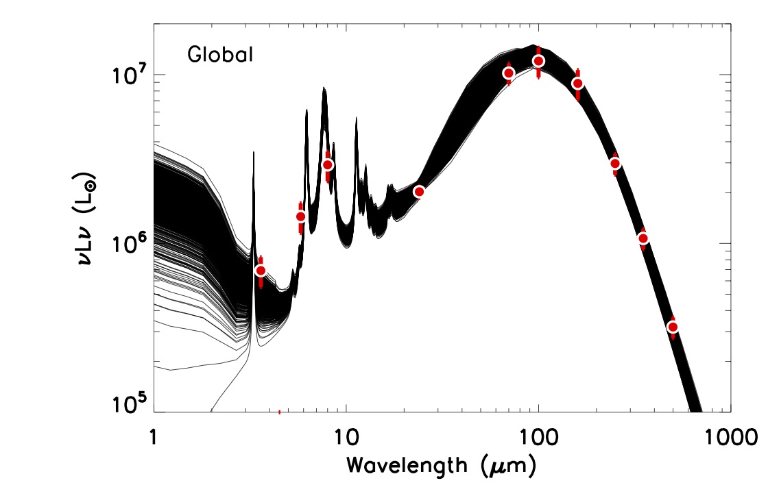
Figure 3: The global SED and 2 local SEDs (from one ISM element in N11B and one element from the more quiescent ISM) modeled with the Galliano et al. (2011) ‘AC’ model. The various lines show the different realizations of the Monte Carlo technique we use to determine the parameter uncertainties (1000 realizations for each of these 3 cases). Herschel measurements are overlaid in red.

The free parameters of our model are thus:

• the total mass of dust (M_dust),

• the PAH-to-dust mass ratio (f_PAH),

• the index of the intensity distribution ($\alpha$),

• the minimum heating intensity (U_min),

• the range of starlight intensities (U),

• the mass of old stars (M_oldstars).

We apply the model to the Spitzer+Herschel dataset (3.6 to 500 $\mu$m) and convolve it with the instrumental spectral responses of the different cameras in order to derive the expected photometry. The fit is performed using a Levenberg-Marquardt least-squares procedure and uncertainties on flux measurements are taken into account to weight the data during the fitting (1 / uncertainty² weighting). The Galliano et al. (2011) model can help us to quantify the total infrared luminosities (L_TIR) across the region. The model also predicts flux densities at longer wavelengths than the SPIRE 500 $\mu$m constraint. We will, in particular, use predictions at 870 $\mu$m in order to decompose the observed 870 $\mu$m emission into its various (thermal dust and non-dust) components in $\S$4.5.

Modified blackbodies (MBB) models are commonly used in the literature to obtain average dust temperatures. In order to relate the temperatures derived using this method with the radiation field intensity derived from the more complex Galliano et al. (2011) fitting procedure, we fit the 24-to-500 $\mu$m data using a two-temperature model, i.e. of the form: L_ν = A_warm $\lambda$^-2 B_ν($\lambda$, T_warm) + A_c $\lambda$${}^{-\beta_{cold}}$ B_ν($\lambda$, T_cold). In this equation, B_ν is the Planck function, T_warm and T_cold are the temperature of the warm and cold components, $\beta$_cold is the emissivity index of the cold dust component and A_warm and A_cold are scaling coefficients. We follow the standard approximation of the opacity in the Li & Draine (2001) dust models for the warm dust component (emissivity index of the warm dust fixed to 2). We fix the emissivity index of the cold component $\beta$_cold to the average value derived for the LMC in Planck Collaboration (2011), i.e. 1.5. Fixing $\beta$ allows us to minimize the degeneracies between the dust temperature and the emissivity index linked with the mathematical form of the model we use and limit the biases resulting from this degeneracy (Shetty et al., 2009; Galametz et al., 2012). Potential variations in the grain emissivity across the N11 complex (so using a free $\beta$_cold) are discussed in $\S$5.3.4.

3.2 Deriving the parameter maps and median local SEDs

We run the SED fitting procedures for elements with a 2-$\sigma$ detection in all the Herschel bands. We apply a Monte Carlo technique to generate for every ISM element 30 local SEDs by randomly varying the fluxes within their error bars with a normal distribution around the nominal value. A significant part of the uncertainties in SPIRE bands is correlated. To be conservative in the parameters we derive, especially on the dust mass estimates directly affected by variations in the SPIRE fluxes, we decide to link the variations of the three SPIRE measurements consistently during the Monte Carlo procedure. Figure 3 shows an example of Monte Carlo realizations of the Galliano et al. (2011) ‘AC’ modeling procedure in three cases: if we consider the N11 complex as one single ISM element (top), for one ISM element in N11B (middle) and for a more quiescent ISM element (bottom). We finally use these various local Monte Carlo realizations to create a median map for each parameter and a median SED for each 14″ $\times$ 14″ ISM elements. The standard deviations are also providing the uncertainties on each of the parameter derived from the modeling. The parameter maps are discussed in $\S$4.

3.3 Residuals from the Galliano et al (2011) fitting procedure

In order to assess the ability of the Galliano et al. (2011) procedure to reproduce the observations, we analyze the residuals to the fitting procedure at i = 8, 24, 70, 100, 160, 250, 350 and 500 $\mu$m. In order to obtain a synthetic photometry (L${}_{\nu}^{modeled}$(i)) to which observed fluxes (L${}_{\nu}^{observed}$(i)) can be compared directly, we integrate the median modeled SEDs obtained on local scales in each instrumental filter. Recall that all these observed fluxes are included as constraints in the fitting process. The relative residuals r_i determined in this study are defined as:

$$r_{\rm i}=\frac{L_{\rm\nu}^{observed}(i)-L_{\rm i}^{modeled}(i)}{L_{\rm\nu}^{observed}(i)}$$ (1)

Figure 4 (top) compares the spatial distribution of the relative residuals of r₈, r₂₄, r₇₀, r₁₀₀, r₁₆₀, r₂₅₀, r₃₅₀ and r₅₀₀ across the N11 complex while Figure 4 (bottom) shows these residuals as a function of the respective flux densities. Relative residuals are quite small. Except for the 160 $\mu$m band, the median values are close to 0, so consistent with a reliable fitting of the observational constraints. The lowest residuals appear in the 24 $\mu$m and the 3 SPIRE (250, 350 and 500 $\mu$m) bands, with standard deviations lower than 0.03. The 70 $\mu$m residual map shows that our modeling procedure slightly underestimates the 70 $\mu$m observed flux in the diffuse regions of N11. This could be linked with emission from VSGs produced through processes of erosion of larger grains in the diffuse medium where they are less shielded from the interstellar radiation fields (Bot et al., 2004; Bernard et al., 2008; Paradis et al., 2009). Residuals in the 100 $\mu$m band seems to be dependent on the ISM element surface brightness (overestimation at low surface brightnesses, underestimation at high surface brightnesses).

The largest residuals are observed in the PACS 160 $\mu$m band, with an underestimation of the observed fluxes by 16% throughout the complex. A non-negligible fraction of these residuals could originate from the strong [C ii] line emission at 157 $\mu$m emitting near the peak of the PACS 160 $\mu$m filter sensitivity. [C ii] emission is indeed detected in every LMC regions mapped with PACS. We estimate that a C ii-to-TIR ratio of 2-3% would be sufficient to explain most of the residual we observe at 160 $\mu$m. This ratio is high but consistent with the values estimated in the N11 complex by Israel & Maloney (2011).

Part of the discrepancies at 100 and 160 $\mu$m could finally be due to a combination of both observational and modeling effects. First, calibration uncertainties in the PACS maps at low surface brightnesses as well as uncertainties in background/foreground estimates have a significant impact on the fluxes in the most diffuse regions. We remind the reader that 160 $\mu$m is where the Galactic cirrus peaks while the LMC SED seems to be flatter than that of the Milky Way in the submm regime. We also remind that the modeling procedure we are using assumes AC, thus have a fixed slope of $\sim$1.7 while the Planck Collaboration (2011) results lead to effective emissivities closer to $\sim$1.5 on average for the LMC. The residuals we observe could thus also be a sign of different optical properties.

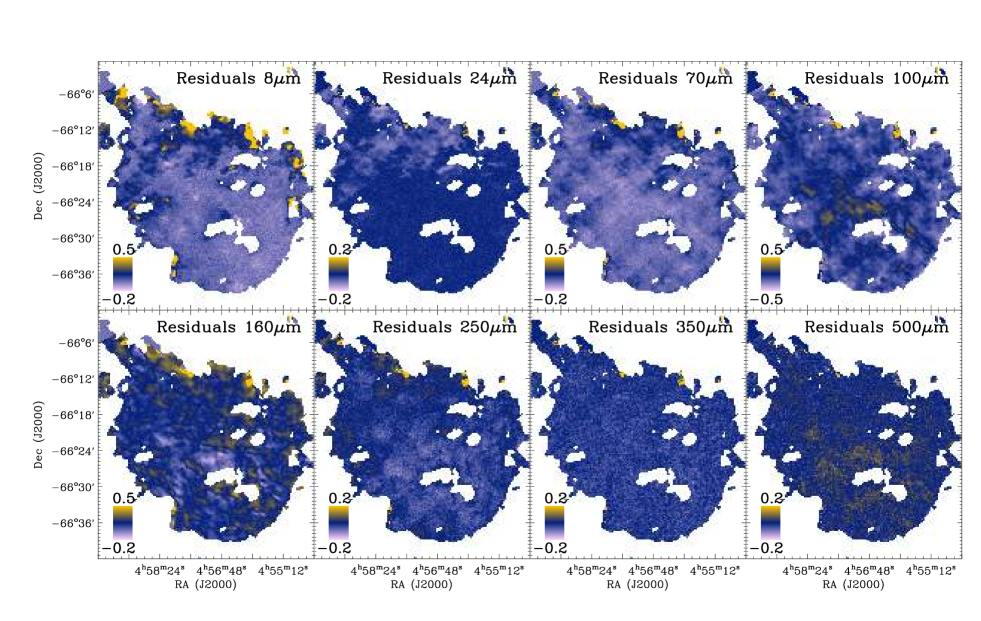
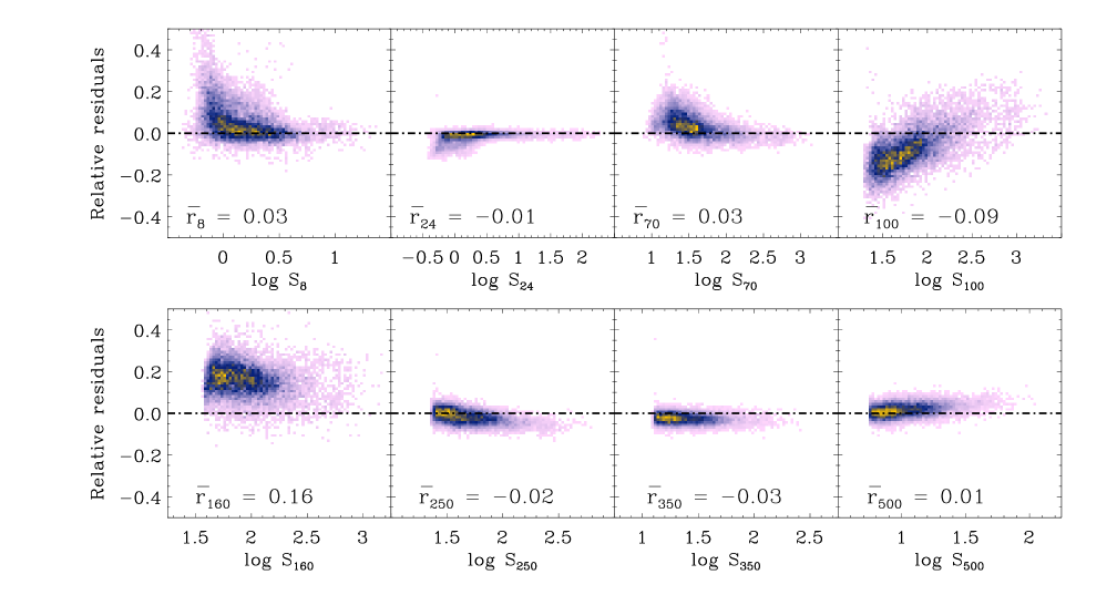
Figure 4: Top - Distribution of the relative residuals r₈, r₂₄, r₇₀, r₁₀₀, r₁₆₀, r₂₅₀, r₃₅₀ and r₅₀₀ to the Galliano et al. (2011) fitting procedure across the N11 complex. The relative residuals are defined as (observed flux - modeled flux) / (observed flux). A residual of 0.2 thus indicates that the model underestimates the observed luminosity by 20%. Bottom - Relative residuals to the Galliano et al. (2011) fitting procedure as a function of the respective observed fluxes S_i. S_i is expressed in MJy/sr. In this plot, colors scale with the density of points. The median value of the residuals is indicated at the bottom of each plot.

4 The dust properties in N11

In this section, we examine local IR-to-submm SEDs across the complex. We also analyze the distributions of the modeling parameters derived from the two SED modeling procedures and their correlations. For the rest of the paper, observed maps and parameter maps will be displayed using two different color tables.

4.1 Local SED variations

Figure 5 (bottom panel) gathers a collection of local IR-to-submm SEDs across the N11 region. These SEDs are extracted from ISM elements located along the north-eastern filament down to the northern edge of the N11 ring (the location of the selected elements is indicated with a white line in the top panel of Fig 5). We can see how the local SED varies from star-forming regions to more quiescent regions. Bright star forming regions (in yellow) show a wider range of temperatures (broader SED) and a lower PAH fraction (weaker features at 8 $\mu$m) while more quiescent regions (in purple) show colder temperatures and a much narrower range of dust temperatures.

From our local modeling of the IR SEDs, we can derive a map of the infrared luminosity L_IR. We integrate the models (in a $\nu$-f$\nu$ space) from 8 $\mu$m to 1100 $\mu$m. The stellar contribution to the near-IR emission was estimated during the SED modeling process. Even if minor in that wavelength range, this contribution is removed from the total L_IR to only take the emission from dust grains into account. Figure 6 (bottom left panel) shows the L_IR map (in units of $L_{\odot}$). We can observe that the distribution of L_IR is much more extended than the regions where high-mass star formation is taking place, with a significant contribution arising from more quiescent regions (regions of weaker 24 $\mu$m emission). This extended distribution is due to the fact that part of the dust emission is not directly related to star formation occurring in the same beam. A fraction of the dust heating is in fact related to the older stellar populations or to ionizing photons leaking out the H ii regions due to the porous ISM in N11 (see Lebouteiller et al., 2012).

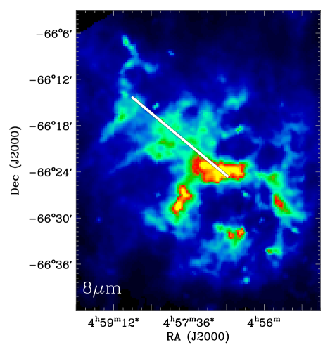
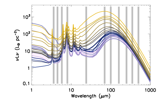
Figure 5: Top: The N11 complex observed in the 8 $\mu$m band. The image has been convolved to the working resolution of 36″. The white line indicates the locations of the ISM elements whose individual SEDs are plotted in the figure below. Bottom: Local SEDs across the N11 complex. Colors indicate the position along the above white line, from light purple in the diffuse ISM (north-east) to yellow in the bright star forming region N11B. The vertical grey lines indicate the position of the Spitzer and Herschel bands.

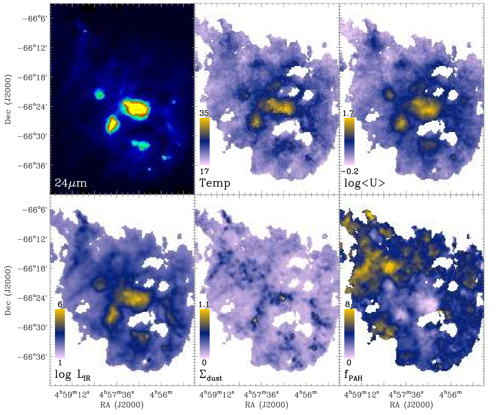
Figure 6: Maps of the parameters derived from our two SED modeling techniques. The 24 $\mu$m map (convolved to a resolution of 36″) is shown for reference in the upper left panel (square root scaling). Top middle panel: Cold dust temperature in Kelvins. Top right panel: Mean starlight heating intensity, with U=1 corresponding to the intensity of the solar neighborhood (log scale). Bottom left panel: Far-infrared luminosity in $L_{\odot}$ pc^-2 (log scale). Bottom middle panel: Dust surface density in $M_{\odot}$ pc^-2. All the parameter maps are obtained using the Galliano et al. (2011) modeling technique (with the choice of amorphous carbon grains to model the carbon dust) except the cold dust temperature map that is obtained using the two-temperature modified blackbody fitting technique.

Bottom right panel: PAH fraction to the total dust mass (in $\%$).

4.2 Radiation field and dust temperatures

Figure 6 (upper middle panel) shows the average cold temperature maps obtained using the MBB model. Temperatures vary significantly across the N11 complex and range from 32.5 K in the N11B nebula (associated with the LH10 stellar cluster) down to 17.7 K in the diffuse ISM (with a median of 20.5 K for regions detected at a 2 but not 3-$\sigma$ level). The median temperature of the modeled regions is 21.5$\pm$2.1 K. This value is similar to that derived if we keep the emissivity index $\beta$ free in the modeling (21.4$\pm$3.4 K). For comparison, Herrera et al. (2013) estimated a mean temperature of $\sim$20 K in the region of N11 from the LMC temperature map of Planck Collaboration (2011), close to what we obtain. The N11 region is representative of the average dust temperatures found in the LMC (Bernard et al., 2008). A comparison between N11 and the N158-N159-N160 star forming complex previously studied by Galametz et al. (2013) shows that N11 is colder on average (median temperature of 26.9 K for the N159 region). The coldest temperatures in the N159 complex were estimated in the N159 South region ($\sim$22 K), a significant reservoir of dust and molecular gas but with no ongoing massive star formation detected. The temperatures of the cold dust grains in the diffuse ISM in N11 are similar to those in N159 South. We finally note that the temperature of N11 when considered as one single ISM element (Fig. 3 top) is 23.1$\pm$1.1 K (at the higher end of the uncertainties of the median derived locally). This highlights again that determining the dust temperatures on local scales is essential to constrain the coldest phases of the dust.

From the Galliano et al. (2011) SED modeling results, we locally derive three parameters characterizing the distribution of the radiation field intensities, namely the index of the simple power law assumed for the distribution $\alpha$ and the minimum and maximum values of the intensities, U_min and U_max respectively. These 3 parameters are combined to derive a map of the mass-weighted mean starlight intensity $<$U$>$ (see Galliano et al., 2011, eq. 11) shown in Fig. 6 (upper right panel). Recall that values are normalized to those of the solar neighborhood (with U = 1 corresponding to an intensity of 2.2 $\times$ 10^-5 W m^-2). The dust temperature of the cold grains (derived from the MBB modeling) and the mean radiation field intensity $<$U$>$ that heat those grains (derived from the ‘AC model’) have very similar distribution, as expected. While we analyze the local and median values of these two parameters in this section, their correlation is studied in more details in $\S$4.4. The median intensity $<$U$>$ of the N11 complex is 2.3 (2.8 if we restrict the median calculation to regions with a 3-$\sigma$ detection in the Herschel bands). Peaks in the $<$U$>$ distribution are observed along the N11 shell, in particular in the N11B nebula where it reaches a maximum of 31.8 times the solar neighborhood value. This value is similar to that estimated in the LMC/N158 region in Galametz et al. (2013). N158 is a H ii region where two OB associations were detected (Lucke & Hodge, 1970). In N158, the southern association hosts two young stellar populations of 2 and 3-6 Myr (Testor & Niemela, 1998). These cluster ages are close to those expected from the intermediate-mass Herbig Ae/Be population detected in the N11B nebula by Barbá et al. (2003). The two regions are thus very similar in terms of evolutionary stage.

4.3 The dust distribution

4.3.1 Total dust masses

Figure 6 (bottom middle panel) shows the surface density map $\Sigma$_dust (units of $M_{\odot}$ pc^-2) obtained with the ‘AC model’. The dust distribution appears to be very structured and clumpy, with major reservoirs in N11B as well as in the N11C nebula located on the eastern rim. Secondary dust clumps are located along the N11 shell. The median of the dust surface density across N11 is 0.22 $M_{\odot}$ pc^-2. The total dust mass derived for the complex is 3.3$\pm$0.6 $\times$ 10⁴ $M_{\odot}$. Uncertainties are the direct sum of the individual uncertainties derived from our Monte-Carlo realizations. The main peaks in the dust distribution coincide with the molecular clouds catalogued by Herrera et al. (2013, identification on the SEST CO(2-1) observations at a 23″ resolution) as shown later in Fig. 9 (bottom panel). We find that only 10$\%$ of the total dust mass ($\sim$2.7$\pm$0.5 $\times$ 10³ $M_{\odot}$) resides in these individual clumps.

Using the same dataset than this analysis and a single temperature blackbody modified by a broken power-law emissivity (BEMBB), Gordon et al. (2014) produced a dust mass map of the whole LMC. They obtain a total dust mass that is a factor of 4-5 lower than values derived from standard dust models like the Draine & Li (2007) models. We convolve our $\Sigma$_dust mass map to their 56″ working resolution to position our dust estimates (for the same area) in that dust mass range. We find that the mass estimated for the whole N11 region in Gordon et al. (2014) is 2.5 times lower than the dust mass we derive (on average 2.4 times lower for $\Sigma$_dust $<$ 0.2 $M_{\odot}$ pc^-2 and 2.6 times lower for $\Sigma$_dust $>$ 0.2 $M_{\odot}$ pc^-2). The dust masses we estimate with the ‘AC model’ are moreover 2.5 times lower than those obtained if we use standard graphite in lieu of amorphous carbon to model the carbonaceous grains (as already shown in Galliano et al. (2011) and Galametz et al. (2013)). Our dust masses thus reside in between those derived by the BEMBB model and a standard ‘graphite’ dust model. These results highlight how the choice of dust composition can dramatically influence the derived dust masses.

Finally, many studies have shown that total dust masses are usually underestimated when derived globally rather than locally (Galliano et al., 2011; Galametz et al., 2012, among others). On global scales, the SED modeling technique is poorly disentangling between warm / cold / very cold dust at submm wavelengths - due to the combined effects of a poor spatial resolution and a small number of submm constraints - and the coldest phases of dust can be diluted in warmer regions. This ‘resolution effect’ is not a physical effect but a methodological bias linked with the non-linearity of the SED modeling procedures. To test this effect in N11, we model the complex as a single ISM element. We obtain a total dust mass of 2.8$\times$10⁴ $M_{\odot}$, thus $\sim$15$\%$ lower than the ‘resolved’ dust mass. This estimate is at the lower limit of our dust mass uncertainty range.

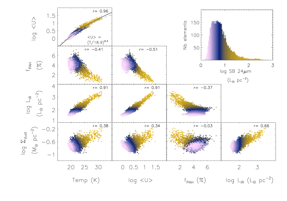
Figure 7: Correlation plots between various model parameters: the dust temperature (Temp) in K, the mean starlight heating intensity normalized to the intensity of the solar neighborhood ($<$U$>$), the PAH-to-total dust mass in percent (f_PAH), the IR luminosity in $L_{\odot}$ (L_IR) and the dust surface density in $M_{\odot}$ pc^-2 ($\Sigma$_dust). All parameters are obtained using the Galliano et al. (2011) modeling technique except the cold dust temperature that is obtained using the two-temperature modified blackbody fitting technique. The Spearman rank correlation coefficients are added to each plot. The ISM elements are colored as a function of their MIPS 24 $\mu$m surface brightness. The inset plot shows the 24 $\mu$m surface brightness histogram and provides the color scale for the plots (from yellow for higher 24 $\mu$m surface brightnesses to light purple for lower 24 $\mu$m surface brightnesses). The grey curve on the top panel indicates the best-fit curve. The equation is provided in the panel. The dashed grey curve indicates the fit with a coefficient fixed to 5.7 ($<$U$>$ = (T/18.6)^5.7).

4.3.2 PAH fraction to the total dust mass

PAHs are planar molecules ($\sim$1nm) made of aromatic cycles of carbon and hydrogen and are thought to be responsible for the strong emission features observed in the near- to mid-IR (Leger & Puget, 1984). The main features are centered at 3.3, 6.2, 7.7, 8.6 and 11.3 $\mu$m. Draine & Li (2007) and Zubko et al. (2004, bare silicate and graphite grain models) found that 4.6$\%$ of the total dust mass in the Milky Way could reside in PAHs. Using Spitzer/IRS spectra, Compiègne et al. (2011) obtain a larger f_PAH (7.7$\%$) for the same environment. It has been shown that the PAH fraction also varies significantly depending on the intensity of the radiation field and with the metallicity of the environment (Engelbracht et al., 2008; Galliano et al., 2008, among others). Our fitting procedure can help us assess these variations on local scales. Figure 6 (bottom right panel) shows the distribution of the PAH-to-total dust mass fraction (in $\%$) across the N11 complex. We find a median f_PAH across the complex of $\sim$4$\%$, thus close to the Draine & Li (2007) and the Zubko et al. (2004) studies. However, the fraction varies significantly across the complex. Lower fractions ($<$1%) are for instance estimated for regions with high radiation field intensities while higher fractions ($>$6-12%) are observed in more diffuse regions of the complex. This is similar to what has been observed in the LMC N158-N159-N160 complex (Galametz et al., 2013) and consistent with the expected destruction of PAH molecules through photodissociation processes scaled with the radiation field hardness and intensity (Madden, 2005).

Caveats - Laboratory experiments have shown that the various PAH bending modes (C-C, C-H etc.) vary with the PAH charge: neutral PAHs preferably emit around 11$\mu$m while ionized PAHs preferably emit around 8 $\mu$m. Because of our lack of constraint in the mid-IR spectrum, we fixed the fraction of ionized PAHs f_PAH+ to 0.5. This means that i) the f_PAH we derive naturally scales, by model construction, with 8 $\mu$m-to-L_IR luminosity ratio (correlation coefficient r=0.91) and ii) the neutral PAHs scale with the ionized PAHs. Yet, by studying local f_PAH in the SMC (12+log(O/H) $\sim$8.0; Kurt & Dufour, 1998), Sandstrom et al. (2012) find that PAHs in the SMC tend to be smaller and more neutral than in more metal-rich environments. This could also be the case in the LMC, affecting the PAH mass. Mid-IR spectra would be necessary to properly quantify the ionized-to-neutral PAH fraction in N11. On a side note, Jones et al. (2013) (see also Jones, 2014) recently proposed nanometer-sized aromatic hydrogenated amorphous carbon grains (a-C(:H)) in lieu of free flying PAHs to explain the mid-IR diffuse interstellar bands we observe in the Galaxy. A more systematic comparison of the two hypotheses would enable us to test their ability to reproduce the observations of different environments.

4.4 Correlations between parameters

Figure 7 presents correlation plots between the dust temperature (Temp), the mean starlight heating intensity ($<$U$>$), the PAH fraction f_PAH, the IR luminosity L_IR and the dust surface density $\Sigma$_dust. We are using ISM elements of 14″, which means that our neighboring pixels are not independent. However, a quick test using 42″ pixels shows that the correlations observed in Figure 7 are not affected by our choice of pixel size.

The top left panel shows the strong relation between the dust temperature and the mean starlight heating intensity across the N11 complex. In thermal equilibrium conditions, the energy absorbed by a dust grain is equal to that re-emitted. This leads to a direct link between the temperature of the grain T, its emissivity $\beta$ and the intensity of the surrounding radiation field U, with U $\propto$ T^(4+β). By model construction, the submillimeter effective emissivity of our “AC model” is $\beta$ = 1.7 (see Galliano et al., 2011), so $<$U$>$ is proportional to T^5.7. We fit our ISM elements, fixing $\beta$ to 1.7, and derive the relation $<$U$>$ = (T/18.6^±0.02)^5.7, thus a normalizing equilibrium dust temperature of 18.6K (dashed line in Fig. 7, top panel). Fitting our ISM elements with no a priori on $\beta$ leads to the relation: $<$U$>$ = (T/18.9^±0.05)${}^{6.4^{\pm 0.10}}$ (solid line). Uncertainties in the fit are calculated using a jackknife technique: we apply the fit to 1/10 ISM elements randomly selected and derive the parameters. We then repeat this procedure 1000 times to derive a final median and standard deviation per parameter. The small uncertainties highlight the very tight correlation between these two parameters. The predicted relation between $<$U$>$, T and $\beta$ is different from that fitted to the ISM elements modeled. This discrepancy is driven by ISM elements with log $<$U$>$ $<$ 0.5, i.e. the ‘diffuse’ ISM of N11. These elements show a very steep submm slope. They reach effective $\beta$ higher than 2 when you let $\beta$ vary, values that are difficult to explain from our current knowledge about grain physics. Because we fix $\beta$ to 1.5 in our MBB fitting technique, our cold temperatures are higher than what would be derived with a higher index (i.e. $\beta$=1.7 or more). This translates into an increase of the fitting coefficient from 5.7 to 6.4.

Figure 7 also shows the close relation between f_PAH and $<$U$>$. f_PAH reaches a constant fraction ($\sim$4%) when $<$U$>$ is lower than $\sim$3. Above this threshold value, we observe a linear decrease of f_PAH with log $<$U$>$. The lower panels in Fig. 7 also show the correlations with $\Sigma$_dust. We do not observe strong variations of column density across the complex. Most of the variations of the IR power are rather driven by the variations in the radiation field intensity. Dense regions have a higher $<$U$>$ and a lower f_PAH, as expected from regions with embedded star formation.

4.5 Dissecting the components of the 870 $\mu$m emission

As explained in $\S$2.3, the data reduction of LABOCA data can lead to a filtering of faint extended emission. If our iterative data reduction procedure helps recover a significant amount of emission around the brighter structures, part of the very extended faint emission (well traced by the Herschel/SPIRE instrument for instance) is not recovered. Only the flux densities in regions with sufficient S/N (i.e. $>1.5$) can then be trusted. For these reasons, we decide not to include the 870 $\mu$m data as a direct constraint in the dust modeling procedure. However, the LABOCA 870 $\mu$m map traces the coldest phases of dust in the complex. By comparing the 870 $\mu$m emission predicted by our dust models (fixed emissivity properties) with the observed 870 $\mu$m emission, it can also help us investigate potential variations in the grain emissivity in the submm regime. We decompose the various contributors to the 870 $\mu$m emission in this dedicated section. Part of the emission at 870 $\mu$m in this particularly massive star forming region is linked with non-dust contributions, namely ¹²CO(3-2) emission line falling in the wide LABOCA passband (at 345GHz) and thermal bremsstrahlung emission produced by free electrons in the ionized gas. We will quantify how much of the measured 870 $\mu$m surface brightness can reasonably be attributed to thermal dust emission, free-free continuum and CO(3-2). This study will allow us to investigate the presence (or not) of any submm emission not explained by these “standard” components (the so-called ‘submm excess’).

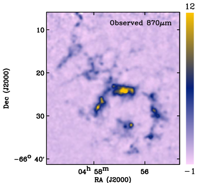
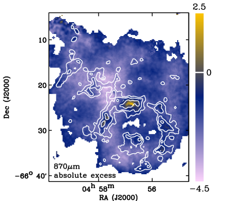
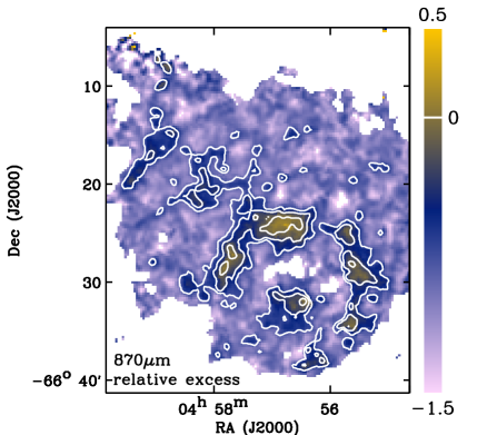
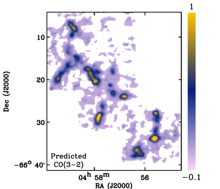
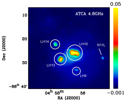
Figure 8: Top left: 870 $\mu$m flux density in MJy sr^-1 observed with LABOCA (resolution of SPIRE 500$\mu$m, i.e. 36″). Top right: 870 $\mu$m flux density in MJy sr^-1 predicted by the AC model, i.e. pure thermal dust emission (same resolution). Middle left: 870 $\mu$m absolute excess in MJy sr^-1 defined as (observed - modeled flux). The modeled flux is that predicted by the AC model (so pure thermal dust emission). LABOCA signal-to-noise contours (S/N = 1.5, 5, 15) are overlaid. Middle right: 870 $\mu$m relative excess defined as ((observed - modeled flux) / modeled flux). Bottom left: CO(3-2) pseudo-continuum flux densities in MJy sr^-1 (resolution: 45″). Bottom right: ATCA radio map at 4.8 GHz (from Dickel et al., 2005) in Jy beam^-1 (original resolution). The positions of the 4 main OB associations in the complex as well as the SNR N11L are indicated. The circles indicate the positions and sizes of the photometric apertures used to derive the fluxes provided in Table 2.

Table 2: IR-to-submm photometry of the OB associations in N11 and non-dust contribution to the 870$\mu$m fluxes

		LH9 / N11F	LH10 / N11B	LH13 / N11C	LH14 / N11E
Center a	(RA)	04h56m35s	04h56m48s	04h57m46s	04h58m12s
	(DEC)	-66∘32′04″	-66∘24′18″	-66∘27′36″	-66∘21′38″
Radius	(arcsec)	100	200	150	120
8 $\mu$m	(Jy)	2.7 $\pm$ 0.3	14.9 $\pm$ 1.5	7.2 $\pm$ 0.7	3.2 $\pm$ 0.3
24 $\mu$m	(Jy)	7.5 $\pm$ 0.7	84.2 $\pm$ 8.4	28.0 $\pm$ 2.8	7.7 $\pm$ 0.8
70 $\mu$m	(Jy)	101.4 $\pm$ 10.1	815.6 $\pm$ 81.6	312.1 $\pm$ 31.2	110.2 $\pm$ 11.0
100 $\mu$m	(Jy)	153.6 $\pm$ 15.4	1220.3 $\pm$ 122.0	507.0 $\pm$ 50.7	190.8 $\pm$ 19.1
160 $\mu$m	(Jy)	162.8 $\pm$ 6.5	968.4 $\pm$ 38.7	456.0 $\pm$ 18.2	193.8 $\pm$ 7.8
250 $\mu$m	(Jy)	76.9 $\pm$ 5.4	416.7 $\pm$ 29.2	212.6 $\pm$ 14.9	102.4 $\pm$ 7.2
350 $\mu$m	(Jy)	38.1 $\pm$ 3.8	191.4 $\pm$ 19.1	102.5 $\pm$ 10.3	50.5 $\pm$ 5.1
500 $\mu$m	(Jy)	16.1 $\pm$ 1.6	77.1 $\pm$ 7.7	42.3 $\pm$ 4.2	21.3 $\pm$ 2.1
870 $\mu$m b	(Jy)	4.2 $\pm$ 0.3	12.2 $\pm$ 0.9	7.1 $\pm$ 0.5	3.1 $\pm$ 0.2
f870,free-free	(%)	7.4	10.4	9.1	6.3
f870,CO	(%)	$<$6	$<$4	$<$20	-

• The photometric apertures are shown in Fig. 8 (bottom right panel).

• Observed flux density not corrected for the non-dust contribution.

4.5.1 Thermal dust emission at 870 $\mu$m and excess maps

From our local SED modeling (the physically motivated “AC model”), we derive a prediction of the pure thermal contribution to the 870 $\mu$m observations. The observed and predicted maps at 870 $\mu$m are shown in Fig. 8 (top panels). Their resolution is our working resolution of 36″. To compare the two maps, we compute the absolute differences between observations and model predictions defined as (observed flux at 870 $\mu$m - modeled flux at 870 $\mu$m) and the relative differences between observations and model predictions defined as (observed flux at 870 $\mu$m - modeled flux at 870 $\mu$m) / (modeled flux at 870 $\mu$m). The maps (that we call the absolute and relative excess maps) are shown in Fig. 8 (middle panels). We overlay the contours of LABOCA S/N to highlight regions where the LABOCA emission is higher than a 1.5-$\sigma$ threshold. The image shows that most of the structures below our S/N threshold correspond to regions where the SED model over-predicts the observed 870 $\mu$m (negative difference). As previously suggested, part of the diffuse emission might be filtered out during the data reduction in these faint regions. In regions above our S/N criterion, the distribution of the relative excess seems to follow the structure of the complex. The observed emission at 870 $\mu$m is close to the predicted value (weak emission in excess) on average and the relative excess reaches $\sim$20$\%$ at most in the center of N11B. We will now try to quantify the non-dust contribution to the 870 $\mu$m flux that could partly account for this excess.

4.5.2 CO(3-2) line contribution

A ¹²CO(1-0) mapping of LMC giant molecular clouds (GMCs) has been performed using the Australia Telescope National Facility Mopra Telescope as part of the Magellanic Mopra Assessment (MAGMA; 45″ resolution) project (Wong et al., 2011). We are using these observations to estimate the ¹²CO(3-2) line contribution to the 870 $\mu$m flux. To do the conversion, we need to assume a brightness temperature ratio R_3-2,1-0. In LMC GMCs, this ratio ranges between 0.3 and 1.4 (average of the clumps: 0.7), with high values ($>$1.0) being associated with strong H$\alpha$ fluxes (Minamidani et al., 2008). They find an average brightness temperature ratio of about 0.9 in the N159 star forming complex. The dust temperature in N11 being lower than that in N159 as shown in $\S$4.2, the R_3-2,1-0 is probably lower than this value. We used the average R_3-2,1-0 ratio of 0.7 derived in Minamidani et al. (2008) to convert the CO(1-0) map into a CO(3-2) map. We use the formula from Drabek et al. (2012) to convert our CO line intensities (K km s^-1) to pseudo-continuum fluxes (mJy beam^-1):

$$\frac{C}{(mJy~{}beam^{-1})(K~{}km~{}s^{-1})^{-1}}=\frac{2k\nu^{3}}{c^{3}}\frac{g_{\rm\nu}(line)}{\int g_{\rm\nu}~{}d\nu}\Omega_{\rm B}$$ (2)

where k is the Boltzmann constant, $\nu$ is the frequency, $\Omega$_B is the telescope beam area, g_ν(line) is the transmission at the frequency of the CO(3-2) line and $\int$ g_ν d$\nu$ is the transmission integrated across the full frequency range. g_ν(345GHz)/$\int$g_ν d$\nu$ is $\sim$0.017 for LABOCA (private communication; G. Siringo, ESO/MPIfR; 2007). The derived CO(3-2) map is shown in Fig. 8 (bottom left). We convolve the 870 $\mu$m map to the resolution of the CO(3-2) map (Gaussian kernel) to compare the two maps. We estimate a contribution of $\sim$15-20$\%$ in LH13, $<$6$\%$ in LH10 and LH9 and from 4 to 12$\%$ in the west ring and in the northern elongated structure detected by LABOCA. We note that LH14 is not fully covered in the public MAGMA map we are using. These values are reported in Table 2.

4.5.3 Free-free contribution

Figure 1 shows the H$\alpha$ distribution (whose distribution should be co-spatial with that of the free-free component across the complex) while Fig. 8 (bottom right) presents a mosaicked image of the 4.8 GHz radio continuum emission taken with the Australia Telescope Compact Array (ATCA). The radio (ATCA) maps at 4.8 and 8.6 GHz (resolution of 33″ and 20″ respectively) obtained from Dickel et al. (2005) are used to model the free-free emission where radio emission is detected. We first convolve the two maps to the working resolution of 36″ using a Gaussian kernel. We then estimate the 870 $\mu$m, 6.25 and 3.5 cm flux densities in the 4 OB associations of the complex (LH9, LH10, LH13 and LH14) shown in Fig. 8 (middle). The circles indicate the positions and sizes of the photometric apertures. The 8 to 870 $\mu$m flux densities in the 4 individual regions are provided in Table 2. We use the two ATCA constraints to extrapolate the free-free emission in the 870 $\mu$m band, assuming that the free-free flux density is proportional to $\nu$^-0.1. We estimate free-free contributions of 10.4, 9.1, 7.4 and 6.3$\%$ in LH10, LH13, LH9 and LH14 respectively. These values are reported in Table 2.

Potential synchrotron contamination - In this analysis, we assume that the radio emission across the complex is dominated by free-free emission. However, radio continuum observations can trace both thermal emission from H ii regions and synchrotron emission. Polarized synchrotron emission can, for instance, be produced in supernova remnants (SNRs). This is the case in particular for the SNR N11L detected in the ATCA observations and indicated in Fig. 8. This SNR is however located outside the regions where the 870 $\mu$m excess peaks. Synchrotron radiation can also be an artificial source of X-rays in the ISM. Using X-ray observations of the N11 superbubble from the Suzaku observatory, Maddox et al. (2009) detected non-thermal X-ray emission around the OB association LH9. However, the photon index of the required non-thermal power-law component is too hard to be explained by a synchrotron origin. Our hypothesis of negligible contamination of the 870 $\mu$m emission in N11 by synchrotron emission thus seems reasonable.

4.5.4 Conclusion

The excess above the pure thermal dust emission we observe in $\S$4.5.1 is weak and can be, within uncertainties, accounted for by the various non-dust contributions (CO line emission and free-free emission) we estimated. We conclude that the 870 $\mu$m can fully be reproduced by these 3 standard components.

5 Comparison between the dust and the gas tracers

In this section, we use the dust surface density map we generate to study the relation between the dust reservoir and the gas tracers. We use H i and CO observations to derive an atomic and a molecular surface density map of N11. By studying the variations of the ‘observed’ GDR across the complex, we will be able to explore the influence of each of the assumptions we made.

5.1 The gas reservoirs in N11

5.1.1 Atomic gas

Kim et al. (2003) produced a high-resolution H i data cube of the LMC by combining their ATCA data with observations of the Parkes 64-m radio telescope from Staveley-Smith et al. (2003). The final cube has a velocity resolution of 1.649 km s^-1 and a spatial resolution of 1′. The H i intensity map of the N11 complex was obtained by integrating the data cube over the 190 $<$ v_hel $<$ 386 km s^-1 velocity range. This excludes the galactic contamination caused by the low galactic latitude of the LMC (b $\sim$ -34^∘). We transform this integrated H i intensity map to atoms cm^-2 units assuming that the 21cm line is optically thin across the complex. We discuss potential consequences of this assumption in $\S$5.3.3. We finally fit the distribution of pixels outside the LMC by a Gaussian and subtract the peak value (as a background estimate) from the data. The H i contours (in atoms cm^-2) are overlaid on the dust surface density $\Sigma$_dust map in Fig. 9. N11 is located at the south of a supergiant shell ($\sim$30′ in radius; see Fig. 9) that is expanding at a velocity of 15 km s^-1 (see Kim et al., 2003). A significant reservoir of atomic gas is detected in the complex, in particular in the north-eastern structure delimiting the supergiant shell rim. Compared to the N158-N159-N160 region where the major peaks of the FIR emission systematically reside in H i holes (Galametz et al., 2013), the H i distribution broadly follows the FIR (and dust) distribution in N11. However, the peaks of the H i distribution are not co-spatial with the peaks in the dust mass distribution. The ionized cavity around LH9 is H i free.

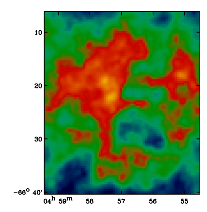
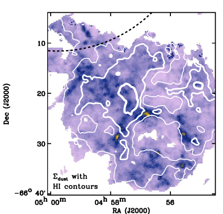
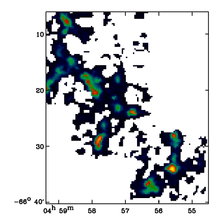
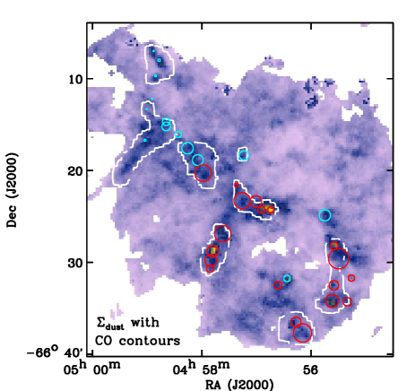
Figure 9: Relation between dust and gas in N11. Top left: H i map of N11. Top right: $\Sigma$_dust map of the complex (units of $M_{\odot}$ pc^-2) with H i contours overlaid. The levels are 3$\times$10²¹, 4$\times$10²¹ and 5$\times$10²¹ atoms cm^-2 (from thinner to thicker lines). The dashed circle indicates the location of the supergiant shell located north to the N11 star forming region. Bottom left: MAGMA CO map of N11. Bottom right: $\Sigma$_dust map of N11 with a MAGMA CO contour at 1.4 K km s^-1 (the survey has a 3-$\sigma$ sensitivity limit of 1.2 K km s^-1). Molecular clouds identified by Herrera et al. (2013) are shown in red. Additional molecular clouds previously identified by Israel et al. (2003) are overlaid in cyan. Both studies have identified molecular clouds based on SEST observations of N11. The radii of the circles indicate the geometrical radii of the clouds fitted to the SEST observations at these positions.

5.1.2 Molecular gas

The CO(1-0) line emission is widely used as an indirect tracer of the H₂ abundance. The 1.4 K km s^-1 contour of the MAGMA CO(1-0) map presented previously in the paper is overlaid on the $\Sigma$_dust map in Fig. 9 (bottom). Israel et al. (2003) also mapped some of the N11 clouds in ¹²CO(1-0) and ¹²CO(2-1) emission lines as part of the ESO-SEST key program (FWHM=45″ and 23″ respectively). Herrera et al. (2013) present a follow-up study using fully sampled maps. Both studies provide catalogues of the physical properties of individual molecular clouds (overlaid in Fig. 9) across the N11 complex. We observe that N11 is composed of many individual molecular clumps that account for a significant part of the CO emission detected in the complex. Most of the peaks in CO correspond to peaks in the dust mass map. The main H i peak resides in-between two CO complexes. This H i / H₂ interface is often observed in the LMC. If molecular clouds are thought to primarily form from global gravitational instabilities, Dawson et al. (2013) have shown that up to 25% of the molecular mass residing in LMC supergiant shells could be a direct consequence of stellar feedback such as accumulation, shock compression mechanisms or ionizing radiation. The H i / H₂ interface we observe in N11 could partly result from the same process at smaller scales (the N11 ring is 4 times smaller in size than the supergiant shell located 0.8^∘ north of N11).

Choice of the X_CO factor  -   In order to build a map of the H₂ column density, we need to convert the intensities of the MAGMA CO(1-0) map into masses. The ‘standard’ X_CO factor in the Solar neighborhood is $\sim$2 $\times$ 10²⁰ cm^-2 (K km s^-1)^-1 (Scoville et al., 1987; Solomon et al., 1987) but has a strong dependence on the ISM physical conditions, especially with metallicity (Bolatto et al., 2013). Because of the lower dust content in low-metallicity objects, the UV photons penetrate deeper into the molecular clouds, leading to a drop in the optical depth and a photo-dissociation of the CO molecule (so less CO emission to trace the same H₂ mass). The X_CO factor is thus usually higher in low-metallicity environments. Indirectly using dust measurements to trace the gas reservoirs, Leroy et al. (2011) derived a X_CO factor of 3 $\times$ 10²⁰ cm^-2 (K km s^-1)^-1 for the LMC. X_CO factors were also estimated from the NANTEN survey of nearly 300 GMCs over the whole LMC (Fukui et al., 1999; Mizuno et al., 2001). They find an average value of $\sim$9 $\times$ 10²⁰ cm^-2 (K km s^-1)^-1. The estimate was then refined to be 7 $\times$ 10²⁰ cm^-2 (K km s^-1)^-1 by improving the rms noise level by a factor of two Fukui et al. (2008). By targeting more specifically the CO clumps of N11, X_CO was estimated to be $\sim$5 $\times$ 10²⁰ cm^-2 (K km s^-1)^-1 in Israel et al. (2003) and $\sim$8.8 $\times$ 10²⁰ $\alpha$_vir^-1 in Herrera et al. (2013), with $\alpha$_vir the virial parameter corresponding to the ratio of total kinetic energy to gravitational energy. In their analysis, Herrera et al. (2013) suggest to use $\alpha$_vir$\sim$2 (this leads to a X_CO factor of 4.4 $\times$ 10²⁰ cm^-2 (K km s^-1)^-1). In our analysis, we decide to use the statistically robust average from the whole MAGMA GMC sample obtained by Hughes et al. (2010), i.e. 4.7 $\times$ 10²⁰ cm^-2 (K km s^-1)^-1. This assumes that $\alpha$_vir=1. We will call this value the MAGMA X_CO factor. We note that in the case of an $\alpha$_vir equal to 2, the X_CO value will be close to the Galactic X_CO (4.7 / 2 = 2.35). As a comparison, we will thus also present the results obtained when a standard Galactic X_CO factor is used. We discuss the consequences of these choices further in $\S$5.3.1.

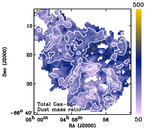
Figure 10: Total gas-to-dust mass ratio map derived at a 1′ resolution. $\Sigma$_dust contours at 0.2, 0.35 and 0.5 $M_{\odot}$ pc^-2 are overlaid (same resolution). The total gas is equal to 1.36 M_HI + M_H2. The molecular mass is estimated from CO(1-0) observations and using an X_CO factor of 4.7 $\times$ 10²⁰ cm^-2 (K km s^-1)^-1 (Hughes et al., 2010). The corresponding probability distribution of the GDR is shown on the right panel. The vertical red line indicates the Galactic total GDR value (i.e. 158; Zubko et al., 2004). The inset shows the histogram of ISM elements not normalized. Regions for which we have CO coverage (thus molecular information) are overlaid in darkgrey.

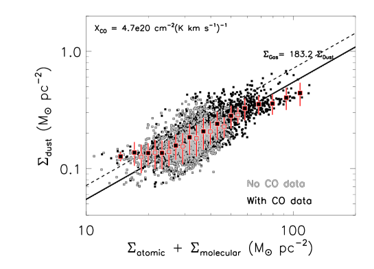
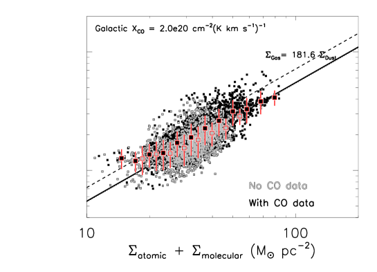
Figure 11: Dust surface density as a function of the total gas surface density. The molecular mass is estimated using an X_CO factor of 4.7 $\times$ 10²⁰ cm^-2 (K km s^-1)^-1 on the left panel and a Galactic X_CO factor of 2.0 $\times$ 10²⁰ cm^-2 (K km s^-1)^-1 on the right panel. On both plots, black points are ISM elements where MAGMA CO data is available and grey points where MAGMA CO data is not available. The larger squares overlaid over the individual ISM elements indicate the averaged $\Sigma$_dust per bins of $\Sigma$_gas (we choose regular bins in logarithmic scale). The linear fit to the pixel-by-pixel relation (in the shape of $\Sigma$_gas = GDR $\times$ $\Sigma$_dust) is indicated for the whole sample with the black solid line, for ISM elements with $\Sigma$_dust $<$ 0.2$M_{\odot}$pc^-2 with the dotted line and for ISM elements with $\Sigma$_dust $>$ 0.2 $M_{\odot}$pc^-2 with the dashed line.

5.1.3 Surface density maps of the gas

The MAGMA CO map at a 1′ resolution (that of the H i map) is already provided on the MAGMA website. We regrid this map and the H i map to a final pixel grid of half the resolution of the H i map, i.e. 7 pc at the distance of the LMC. We derive the H i surface density map ($\Sigma$_HI) and the H₂ surface density map ($\Sigma$_H2) by dividing the local H i masses (M_HI) and the local H₂ masses (M_H2) by the area of our reference pixel (final units: $M_{\odot}$ pc^-2). We multiply the $\Sigma$_HI map by 1.36 to take the presence of helium into account. The MAGMA X_CO factor being derived from virial masses, our $\Sigma$_H2 map includes all the material contributing to the dynamical mass of the cloud, thus already includes helium (this contribution is added however in the Galactic X_CO case). The two final maps will be respectively referred to as the atomic and molecular gas surface density maps $\Sigma$_atomic and $\Sigma$_mol,CO, their sum as $\Sigma$_gas. Assuming that the region follows the Kennicutt (1998) relation ($\Sigma$_SFR = 2.5 $\times$ 10^-4 ($\Sigma$_gas)^1.4), we can use the $\Sigma$_gas map to derive local estimates of the SFRs. For the regions detected at a 2-$\sigma$ level in the Herschel bands, the SFR ranges from 4.5 $\times$ 10^-3 to 2.4 $\times$ 10^-1 $M_{\odot}$ kpc^-2 yr^-1, with an average $\Sigma$_SFR of 4.4 $\times$ 10^-2 $M_{\odot}$ kpc^-2 yr^-1 across the whole complex. Using YSO candidates in the N11 region, Carlson et al. (2012) estimated the SFR in the region to be between 1.8 and 8.8 $\times$ 10^-2 $M_{\odot}$ kpc^-2 yr^-1 (depending on the timescale selected for the Stage i formation, i.e. for embedded sources). The value we estimate from the gas mass is consistent with that SFR range.

5.2 Relations between dust and gas surface densities

We convolve the $\Sigma$_dust map (resolution: 36″) to the resolution of the $\Sigma$_gas map using Gaussian kernels (same pixel grid). We then derive an ‘observed’ total GDR map of N11. The map obtained using the MAGMA X_CO factor to derive the molecular gas is shown in Figure 10. The corresponding probability distribution is shown in the right panel. The vertical line indicates the Galactic GDR value derived by Zubko et al. (2004) (i.e. 158). The inset compares this distribution with that restricted to the regions covered by the MAGMA public release. The range of $\Sigma$_gas we are probing covers about an order of magnitude. The distribution of GDR broadly follows the dust distribution, with highest values of the GDR observed in the most diffuse regions and lowest values detected toward the H ii regions. H i dominates the local gas masses in many regions of the complex.

Figure 11 shows the relation between the dust surface density and the atomic+molecular gas surface density (MAGMA X_CO case on the left panel and Galactic X_CO case on the right panel). Black points distinguish ISM elements where MAGMA CO data is available in the publicly released map. They represent about 45$\%$ of our ISM elements. Grey points indicate elements for which the CO information is not available. They are identical in both panels. Some of these ‘grey’ elements might have CO emission (but are simply not covered). This is probably the case for regions that possess a non-negligible dust surface density at the top of the “grey cloud” of points. Additional molecular gas would shift these elements and tighten the relation between $\Sigma$_dust and $\Sigma$_gas. The larger squares indicate the averaged $\Sigma$_dust per bins of $\Sigma$_gas (we choose regular bins in logarithmic scale). The error bars indicate the scatter within these $\Sigma$_gas bins. In the $\Sigma$_dust range we are studying here (0.1 $\leq$ $\Sigma$_dust $\leq$ 0.5 $M_{\odot}$pc^-2), the relation between $\Sigma$_dust and $\Sigma$_gas seems to be linear. In the case of the MAGMA X_CO factor, we observe a flattening of the relation above $\Sigma$_gas=60 $M_{\odot}$pc^-2. The flattening resides within the error bars in the Galactic X_CO case.

We take the uncertainties on the individual $\Sigma$_dust into account to derive the linear scaling coefficients linking the dust surface densities to the gas surface densities (so to derive the error-weighted averaged GDR of the sample). The thick line in the plots of Fig. 11 indicates these relations. We see that the GDR of the whole region is close to 180 in both X_CO cases. How does this compare to the expected GDR in the LMC (12+log(O/H)=8.3-8.4; see Russell & Dopita, 1990)? We can predict this value using the formula of Rémy-Ruyer et al. (2014) for a broken power-law and a X_CO,Z case (i.e. X_CO $\sim$ Z^-2). This leads to a GDR of 350, thus $\sim$50% more than the global ratio we find. To probe the variations of GDR with the dust surface density, we cut our $\Sigma$_dust range in two intervals, estimating the GDR for $\Sigma$_dust $<$ 0.2 $M_{\odot}$pc^-2 (dotted line) and $\Sigma$_dust $>$ 0.2 $M_{\odot}$pc^-2 (dashed line). The values are 186$\pm$12 and 140$\pm$33 respectively in the case of MAGMA X_CO and 184$\pm$12 and 140$\pm$30 respectively in the case of a Galactic X_CO). The GDR thus decreases with the dust surface densities in the N11 complex. This decrease was previously observed in a strip of the LMC in Galliano et al. (2011) or in the recent study of Roman-Duval et al. (2014).

5.3 Discussion on the low ‘observed’ GDR

Our analysis of GDR in N11 lead to values lower than those expected for an environment such as the LMC. We recall that several assumptions have been made to derive this ‘observed’ GDR map: we assume that i) the X_CO factor is constant across the complex, ii) the CO traces the full molecular gas reservoir, iii) the H i line is optically thin in the region and iv) the dust composition does not vary across the complex. In the following section, we discuss the impact of these hypotheses on the derived GDR and analyse the possible origin of its decrease with the dust surface density.

5.3.1 Underestimation or variations in the X_CO factor

The CO molecule can be highly photo-dissociated in the outer regions of molecular clouds while H₂ is shielded by dust or self-shields from UV photodissociation. As mentioned in $\S$5.1.2, this effect often translates into higher X_CO factors between the observed CO intensities and the H₂ abundance they trace in porous media submitted to strong radiation fields such as N11. In this analysis, we conservatively choose the MAGMA factor derived for GMCs across the LMC, factor that is already 2.4 times higher than the Galactic X_CO factor. However, given the intense radiation fields arising from the multiple OB associations in N11, the X_CO factor could be above the mean MAGMA value that is driven by less energetic environments. Israel (1997) for instance suggests a X_CO factor of 6 $\times$ 10²⁰ cm^-2 (K km s^-1)^-1 in the northeast filament of N11 and of up to 2.1 $\times$ 10²¹ cm^-2 (K km s^-1)^-1 in the N11 ring itself.

Let’s assume a constant GDR of 350 across the region. Which conversion factors would then be required to reach this value? X_CO would be equal to (350 $\times$ $\Sigma$_dust - $\Sigma$_HI) / I_CO. Figure 12 shows the map of the X_CO factors we obtain. Because low signal-to-noise pixels around the edge of the CO-bright clouds are very dependent on the baselines and the signal identification method used to generate the MAGMA CO map, we choose to limit this study to regions above the 3-$\sigma$ sensitivity limit of the MAGMA survey. We observe the highest X_CO values near the bright OB associations LH10 and LH13 and in the northeastern filament. The derived X_CO factor can vary by an order of magnitude: it ranges between 5.2 $\times$ 10²⁰ cm^-2 (K km s^-1)^-1 and 4.9 $\times$ 10²¹ cm^-2 (K km s^-1)^-1, with a mean value of 1.3 $\times$ 10²¹ cm^-2 (K km s^-1)^-1. The minimum factor we obtain is consistent with our nominal (MAGMA) choice for X_CO but using a higher X_CO factor would indeed increase the local GDR values toward the expected LMC GDR in most of these regions. The maximum X_CO factor we find is twice the value estimated for the ring by Israel (1997). Even if possible, these very high X_CO factors are, nevertheless, expected in more extreme environments than the LMC, such as the dwarf irregular galaxies NGC 6822 or the Small Magellanic Cloud (Leroy et al., 2011). A modification of the X_CO factor alone is probably not sufficient to fully explain the low ‘observed’ GDR.

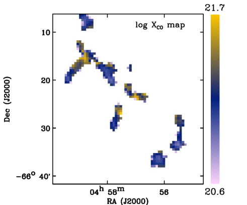
Figure 12: Local variations of the X_CO factor estimated using a constant GDR = 350 across the complex. Units are in cm^-2 (K km s^-1)^-1 (log scale). We limit the study to ISM elements above the 3-$\sigma$ sensitivity limit of the MAGMA CO(1-0) map.

5.3.2 CO-dark gas

Studies tracing gas through the dust emission or the gamma rays emission (produced through cosmic ray collisions in the Galaxy; see Grenier et al., 2005; Ackermann et al., 2012) have highlighted the presence of H₂ that is not detectable through CO observations. This molecular phase, called the “CO-dark” phase is particularly difficult to quantify and can not be related to the CO-emitting reservoirs through the usual X_CO factor. If we consider that this ‘missing molecular phase’ is responsible for the low GDR observed in N11, we can quantify its abundance by doing $\Sigma$${}_{dark~{}gas}$ = 350 $\times$ $\Sigma$_dust - $\Sigma$_HI - $\Sigma$_mol,CO, with $\Sigma$${}_{dark~{}gas}$ the surface density of the molecular dark gas not traced by CO. Before continuing with this analysis, we need to take into account the fact that in the more quiescent regions of the complex, part of the missing gas mass could be already linked with our lack of CO constraints due to the limited coverage of the public MAGMA map. If we assume a constant GDR of 350 throughout the complex, $\sim$ 8.6 $\times$ 10⁵ $M_{\odot}$ are missing from the total gas budget in the regions with no CO data (see Fig. 8 bottom left). We use the good correlation between $\Sigma$_dust and $\Sigma$_mol,CO in the regions covered in CO (Spearman coefficient r=0.5 and $\Sigma$_dust = 0.16$\pm$0.007 $\Sigma$_mol,CO^0.19±0.02) to estimate the CO-emitting molecular gas in the regions not covered in CO. Using this completed $\Sigma$_mol,CO map, we can then derive the mass of the dark gas in the region. We find a fraction of the dark gas to the total gas mass equal to 55-60%. The fraction of the dark gas to the total molecular mass (f_DG = M${}_{dark~{}gas}$ / (M${}_{dark~{}gas}$+M_mol,CO)) is equal to 70-80%, with larger values outside the dust peaks of N11. By theoretically model the dark component, Wolfire et al. (2010) predict that f_DG would be relatively invariant with the incident UV radiation field strength ($\sim$0.3 in the Galaxy for instance) but that this value could increase with i) a decreasing visual extinction and ii) a decreasing metallicity. If our results are consistent with these trends, the very high f_DG fraction we obtain is pushing the models to the limits. This suggests that a hidden reservoir of CO-dark gas is probably not the unique explanation to the low ‘observed’ GDR throughout N11.

We note that further observations would be needed to correctly estimate the CO-faint phase in the complex. The CO-dark reservoirs could also be quantified using the [C ii] 157 $\mu$m line as suggested by Madden et al. (1997). Several studies have indeed shown that the [C ii] emission is more extended than that of CO (Israel & Maloney, 2011; Lebouteiller et al., 2012).

5.3.3 Optically thick HI

The H i column density N_HI can be estimated from the measured H i brightness temperature T_B and the optical depth $\tau$ using equation 3-38 from Spitzer (1978):

$$N_{HI}=1.823\times 10^{18}\int{T_{B}\frac{\tau}{1-e^{-\tau}}d\varv}$$ (3)

where T_B is the measured brightness temperature (K), $\tau$ is the optical depth and $\varv$ is the velocity. In this analysis, we assume that the 21cm line is optically thin across the complex in order to derive the local H i masses. This reduces the equation to N_HI,thin = 1.82 $\times$ 10¹⁸ $\int$ T_B $\tau$ d$\varv$. However, because the H i optical depth strongly depends on N_HI, the assumption of optically thin H i starts to be questionable for large column densities. Recent studies have proposed optically thick H i envelope around CO clouds to explain the large scatter in the relation between the H i velocity integrated intensity and the submm dust optical depth (see Fukui et al., 2014, 2015, for instance). In their study of the Perseus molecular cloud, Lee et al. (2012) estimated the optical depth effects to be responsible of an underestimation of the H i mass by a factor of 1.2-2. Using Eq. 3-37 from Spitzer (1978) and a single spin temperature of T_s = 60K, we estimate that we would need an H i column density of about 10²⁰ cm^-2 per km/s to reach $\tau$ = 1. If we consider a H i line width of $\sim$14km/s (mean value of the H i line width toward the position of the GMCs; Fukui et al., 2009), this leads to a N_HI threshold of 1.4 $\times$ 10²¹ cm^-2 above which optical depth effects could be expected, which is mostly the case in the N11 complex we are studying here. Moreover, several surveys (Dickey et al. (1994) and Marx-Zimmer et al. (2000)) targeting absorption features in compact radio continuum sources toward the LMC have shown that its cold atomic gas is probably colder than that of the Milky Way (down to T_s$\sim$30 K). The theoretical N_HI threshold we determine could thus be even lower in N11. However, Marx-Zimmer et al. (2000) also find that if a few regions such as 30 Doradus and the eastern H i boundary are optically thick, most of the clouds they target in other regions have low values of $\tau$. Unfortunately none of them were in the direction of N11. If present, optically thick H i would lead to an underestimation of the gas masses at high column densities. Higher atomic gas masses in N11 would bring the GDR closer to that expected for a low-metallicity galaxy like the LMC. However, the pixel-by-pixel effect is difficult to quantify. In the N11 complex, the peak in $\Sigma$_dust and $\Sigma$_HI are not co-spatial. As one can see in Fig. 9, $\Sigma$_HI is rather constant around the N11 shell where the $\Sigma$_dust peaks can be found. These regions are going to be less affected by the ‘optically thick’ correction than the northeast filament where the H i distribution peaks. This suggests that the ‘H i optical depth’ effect could only partly explain the low ‘observed’ GDR we find but is not sufficient to explain its progressive decrease with the dust surface densities we obtain.

5.3.4 Dust emissivity variations

The three previous sections were trying to find an explanation of the low ‘observed’ GDR by invoking a modification of the hypotheses made on the gas phase. This section is exploring the hypotheses of a dust abundance variation and their effect on the GDR on local scales. To properly understand the reprocessing of grains in the ISM and quantify the dust abundance variations, one would need to access the intrinsic emissivity of the dust grains. In our local MBB modeling, we fixed the effective emissivity index (i.e. the apparent emissivity index) of the cold dust component to 1.5 in order to minimize degeneracies between the dust temperature and $\beta$. Leaving both parameters free is, however, a commonly used technique to probe potential variations in the dust grain emissivity (see Planck Collaboration et al., 2014b; Tabatabaei et al., 2014; Grossi et al., 2015, ; among many others). So what do we obtain when we let the grain emissivity vary? Figure 13 shows the map of the effective emissivity index derived from a two-temperature modeling of the complex if $\beta$ is used as a free parameter. The median value of the emissivity index $\beta$ is 1.52$\pm$0.19 across the complex if we restrict the analysis to ISM elements with a 2-$\sigma$ detection in the Herschel bands. We note that this median value is consistent with the value we chose to fix in our SED modeling procedure ($\beta$=1.5). Nevertheless, we do observe systematically lower values of $\beta$ (so a flattening of the submm slope) in dense regions compared to the diffuse medium. Part of the explanation could be linked to the fact that the large ISM elements we are studying in this paper contain dust populations with a large range of temperatures. Temperature mixing effects usually lead to shallower observed submm SEDs (Shetty et al., 2009), with the effective emissivity index we observe being, in fact, a non-trivial combination of the intrinsic emissivity index of each dust population. Our SED modeling procedure includes a radiation field intensity range (thus a temperature range) and is able to fit the data up to 500 $\mu$m, suggesting that our assumptions (silicate + AC grains) could be sufficient to explain the submm Herschel fluxes we observe and that flattening of the effective emissivity can be fully explained by temperature gradients in the H ii regions of the complex. The study of the excess at 870 $\mu$m ($\S$4.5) also showed that the residuals we observe at 870 $\mu$m compared to our local SED models (thus compared to ‘pure emission from the cold grains’) could be linked with non-dust contribution from the CO(3-2) line or the free-free emission.

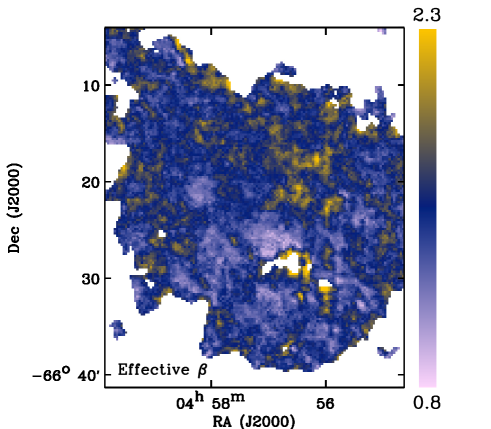
Figure 13: Map of the effective emissivity index of the cold dust grains derived from a two-temperature modeling of the N11 complex. The cold emissivity index $\beta$ is thus considered as a free parameter.

Does this necessarily mean that there is no variation of the dust emissivity index of the grains across the region? The variation of GDR with the dust surface density could suggest otherwise. Indeed, our modeling procedure assumes the same dust grain properties whatever the density in the ISM element we are looking at. However, Roman-Duval et al. (2014) suggested that dust accretion and coagulation processes could be happening in dense phases such as the ones probed in this analysis. If this is the case, this would lead to an overestimation of the dust surface density in environments where the accretion and coagulation processes could occur. A variation of the emissivity index (to lower indices in that particular case) would decrease our estimated dust masses.

5.3.5 Conclusion

As explained in Roman-Duval et al. (2014), it is very difficult to disentangle between the various hypothesis we explore at our working resolution, i.e. the presence of CO dark-gas or real GDR variations with environment, H i optical depth effect or potential variations of the dust abundances. The explanation is probably a combination of all these various effects that affect the GDR in the same direction. Higher resolution observations of the molecular clouds themselves (at much smaller scales than the giant complexes we are mapping here), more specifically a mapping of the submm dust continuum, a sampling of CO spectral line energy distributions, but also observations of other tracers of the dense gas such as HCN or HCO+ with ALMA would be necessary to unambiguously probe the dense clouds and constrain the GDR on small scales in the LMC.

6 A Principal Component Analysis of the IR/submm dataset

In this paper, we have analyzed the local characteristics of dust grains across the star forming region N11. However, the properties we derive are dependent on the assumptions made on the dust composition in the SED modeling technique we have selected. In this last section, the goal would be to explore the capacity of a data processing method based a Principal Component Analysis (PCA) to decompose the various dust populations contributing to the local SEDs in N11 with no a priori on the dust populations.

6.1 Method

The Karthunen-Loève transform, more familiarly called Principal Component Analysis (hereafter PCA), is the orthogonal projection of a set of data into a new system of coordinates. This technique has been used on many astronomical objects and for multiple purposes: analysis of spectral cubes (Mékarnia et al., 2004), reduction of dimensionality for SED libraries (Han & Han, 2014), among many others. Our SED modeling of the N11 complex has enabled us to build a library of spectra across the complex. If we take into account pixels with a 1-$\sigma$ detection in the Herschel bands, this leaves us with 21392 individual dust SEDs. Our goal is to apply a PC decomposition to this multispectral data cube. Using the fully modeled SEDs in lieu of the individual bands provides a much better constraint of the SED shape in each resolution element and will decrease the biases linked with noise in the data. The first step of our analysis is to compute the covariance matrix of the multispectral data cube (we use the IDL function CORRELATE). Since we are mostly interested in the dust SED here, we keep the spectral coverage from 8 $\mu$m to 1000$\mu$m. Each SED in our database is sampled with 117 wavelength points between these two wavelengths. We use the logarithm of our local models to perform the PCA decomposition. From the covariance matrix, we can calculate the eigenvectors and eigenvalues (we use the IDL function EIGENQL, with the covariance option). This directly provides us with an ensemble of vectors that constitute the main building blocks of our local SEDs. The total number of eigenvectors derived in a PCA is equal to the number of spectral elements used for the analysis. We obtain 117 independent eigenvectors. We will only analyze the 6 first eigenvectors in the following analysis. The last step of the analysis is to reconstruct the principal basis images, rotating by the eigenvectors. As we decided to apply a non-standardized PCA (no mean-centering), we expect the first component to mainly correspond to a ‘mean’ SED of the ISM elements while the following components will reflect the deviations from this main SED.

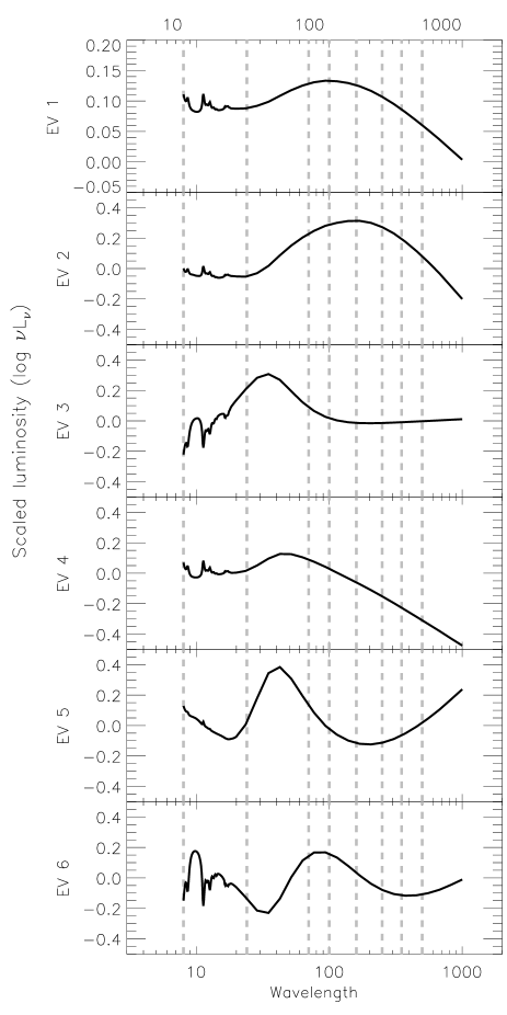
Figure 14: The 6 main eigenvectors. They respectively contain 98.8, 0.53, 0.42, 0.17, 0.06 and 0.02$\%$ of the total variance. The 8, 24, 70, 100, 160, 250, 350 and 500 $\mu$m wavelengths are overlaid as references but the full SED models (sampled with 117 elements) have been used for the decomposition.

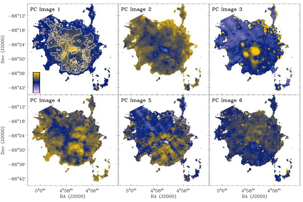
Figure 15: The 6 corresponding component images of the PCA. $\Sigma$_dust contours are overlaid on the first top panel.

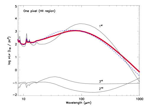
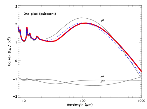
Figure 16: Decomposition of two local SEDs (same pixels as in Fig. 3) using our PCA eigenvectors. The red line shows the 8 to 1000$\mu$m modeled SED and 3 black lines the contribution from the 3 first components (see labels). The dashed line indicates the SED reconstructed from the 3 first components while the dashed-dotted line indicates the SED reconstructed from the 6 first components (those are indistinguishable from the modeled SED).

6.2 Decomposition and interpretation

We find that the first component of the decomposition dominates and contributes to 98.8$\%$ of the total variance in the observed variables (the higher the variance along a given ‘axis’, the more representative the axis). The contributions from the second, third and fourth component rapidly decrease (0.53, 0.42 and 0.17$\%$ respectively). We show the 6 main components/vectors of the PCA in Fig. 14 and the reconstructed PC images in Fig. 15 (color scale from low/purple to high/yellow in the top left panel). An examination of each component allows us to interpret the results of the decomposition process. We observe that the first component (see the vectors in Fig. 14) peaks around 100 $\mu$m: the first basis image (see the PC images in Fig. 15) is, as expected, linked with the bulk of emission arising from the warm/cool regions of the N11 complex and resemble the average SED of the complex. The second component of the PCA peaks around 160 $\mu$m: the second basis image seems to correspond to the contribution of the coldest regions mostly arising outside the N11 ring and filament. The third PCA component peaks between 30 and 40 $\mu$m: the third basis image is thus dominated by the contribution of the hottest regions in the LH14, LH10, LH13 and LH9. We note that in this component, the PAHs are inverted and negative, which is consistent with the fact that PAHs are partly destroyed in H ii regions.

The interpretation of the following PC images is less straightforward. The fourth PCA component peaks around 50 $\mu$m and smoothly decreases toward longer wavelengths: the fourth basis image could thus be related to the hardness of the radiation fields, as it highlights regions where small grains (VSG or PAHs) seems to be excited. This could explain why the distribution of PC4 in Fig. 15 seems to be anti-correlated with the distribution of the dust surface density, the radiation being usually harder in regions of lower optical depth. The fifth component is associated with instrumental noise effects in the MIPS observations (particularly recognizable stripping pattern of the MIPS 70 $\mu$m map). Note that even if we do not include the direct observed 70 $\mu$m map in the PCA, this information seems to be contained in the modeled SEDs. This map thus highlights the non-negligible uncertainties on the dust SED modeling in that part of the spectrum and the power of the PCA approach to derive these small fluctuations. Finally, the sixth basis image is difficult to associate to a specific dust phase. Part of the component could be associated with the old stellar population as peaks in the PC Image 6 are visible toward old stars emitting in the mid-IR. We note that the stellar contribution was not removed from the SED spectra used in this PCA analysis in order to observe its influence on the final SED library.

Figure 16 shows the PC decomposition for two local SEDs (we select the same bright and quiescent pixels as in Fig. 3). The 3 black lines highlight the contribution from the 3 first components (see labels) to the local modeled SED (red line). We overlay the SED reconstructed from the 3 first components with the dashed line and the SED reconstructed from the 6 first components with the dashed-dotted line. This last SED and the reference SED are nearly indistinguishable for both regions. The shape of the first PC component is really similar to the SED shape in the quiescent region. This is expected from the fact that quiescent regions dominate in the complex we are studying. For the ‘warm’ pixel, the contribution from the following components is crucial to account from the warm dust populations and the flattening of the SED shape.

Contrary to many approaches to decompose the local dust SED in nearby objects, the PCA approach has no a priori assumption included in the procedure rather than the information contained in the individual spectra. Our results show quite convincingly that even without a SED modeling procedure, we are able to recover a spatial structure of the different dust populations that has a coherence compared to what we expect for the region. The decomposition of the SED in various dust components (hot, warm, cold) sounds really promising. We will carry out further studies on the full LMC or on a larger sample of galaxies, for instance the KINGFISH survey of nearby galaxies, in order to understand how unique this decomposition is or how it evolves from one environment to another.

7 Conclusions

We combine Spitzer and Herschel data from 3.6 to 500 $\mu$m in order to perform a local dust SED modeling of the N11 massive star forming complex in the Large Magellanic Cloud. We use the amorphous carbon model of Galliano et al. (2011) to derive maps of various grain properties, such as the dust mass or the PAH fraction as well as physical conditions of the ISM (e.g the interstellar radiation field intensity) on scales smaller than 10pc. By performing a careful study of the residuals to the model at all the observed wavelengths, we find non-negligible residuals in the PACS bands, especially at 160 $\mu$m. Part of these local residuals could originate from the strong [C ii] line emission. We also model the data with a more standard two-modified blackbody model to derive local average temperatures and compare them with the radiation field intensity derived from the Galliano et al. (2011). This model also helps us investigate potential variations in the dust emissivity index across N11.

We observe strong local SED variations. We find colder temperatures (on average) than in the LMC N158-N159-N160 star forming complex previously studied by Galametz et al. (2013), with a median temperature of 20.5K. We find a total dust mass of 3.3$\times$10⁴ $M_{\odot}$ in the regions we model. This is a factor of 2.5 times lower than the dust mass derived if we would have used standard graphite to model the carbon dust and a factor of 2.5 higher than the dust masses derived by Gordon et al. (2014) using a BEMBB. The PAH fraction strongly decreases in our H ii regions where they are probably destroyed by the strong radiation fields. We compare our model predictions at 870 $\mu$m with observations obtained with the APEX/LABOCA instrument at the same wavelength. We evaluate the potential non dust contribution to the 870 $\mu$m (CO line, free-free emission) emission. Our local dust SED models provide a satisfying fit of the dust-only emission at 870 $\mu$m.

We relate the dust surface densities to the atomic and molecular surface densities and investigate the variations of the total gas-to-dust ratio across the region. We obtain a low GDR compared to those expected for a low-metallicity environment like the LMC. We also observe a decrease of GDR with increasing dust surface densities. Several effects could be responsible for the variations in the ‘observed’ gas-to-dust mass ratios and we explore the influence of each of the assumptions we made to derive the ratio map. Potential explanations are a variation of the X_CO factor due to the intense radiation fields arising from the H ii regions in N11, the presence of a dark molecular gas component not traced by the available CO observations, the presence of optically thick H i or a variation of the dust abundances in the densest regions of N11. The complete explanation is probably a combination of all these effects that affect the GDR in the same direction.

In the last section, we perform a Principal Component Analysis of the data cube. The first three components allow us to isolate three various dust phases (diffuse medium, cold dust and warm dust) with a spatial structure that is consistent with what we expect for the region. These tests will be extended in future studies to analyze the potential of the PCA method in disentangling the various dust reservoirs for a wider variety of environments.

References

- Ackermann et al. (2012) Ackermann M. et al., 2012, ApJ, 755, 164
- Aniano et al. (2011) Aniano G., Draine B. T., Gordon K. D., Sandstrom K., 2011, PASP, 123, 1218
- Balog et al. (2014) Balog Z. et al., 2014, Experimental Astronomy, 37, 129
- Barbá et al. (2003) Barbá R. H., Rubio M., Roth M. R., García J., 2003, AJ, 125, 1940
- Bernard et al. (2008) Bernard J.-P. et al., 2008, AJ, 136, 919
- Bica et al. (2008) Bica E., Bonatto C., Dutra C. M., Santos J. F. C., 2008, MNRAS, 389, 678
- Bolatto et al. (2013) Bolatto A. D., Wolfire M., Leroy A. K., 2013, ARAA, 51, 207
- Bot et al. (2004) Bot C., Boulanger F., Lagache G., Cambrésy L., Egret D., 2004, A&A, 423, 567
- Calzetti (2007) Calzetti D., 2007, Nuovo Cimento B Serie, 122, 971
- Calzetti et al. (2007) Calzetti D. et al., 2007, ApJ, 666, 870
- Carlson et al. (2012) Carlson L. R., Sewiło M., Meixner M., Romita K. A., Lawton B., 2012, A&A, 542, A66
- Compiègne et al. (2011) Compiègne M., et al., 2011, A&A, 525, A103+
- Dale et al. (2001) Dale D. A., Helou G., Contursi A., Silbermann N. A., Kolhatkar S., 2001, ApJ, 549, 215
- Dawson et al. (2013) Dawson J. R., McClure-Griffiths N. M., Wong T., Dickey J. M., Hughes A., Fukui Y., Kawamura A., 2013, ApJ, 763, 56
- Desert et al. (1990) Desert F., Boulanger F., Puget J. L., 1990, A&A, 237, 215
- Dickel et al. (2005) Dickel J. R., McIntyre V. J., Gruendl R. A., Milne D. K., 2005, AJ, 129, 790
- Dickey et al. (1994) Dickey J. M., Mebold U., Marx M., Amy S., Haynes R. F., Wilson W., 1994, A&A, 289, 357
- Drabek et al. (2012) Drabek E. et al., 2012, MNRAS, 426, 23
- Draine & Li (2001) Draine B. T., Li A., 2001, ApJ, 551, 807
- Draine & Li (2007) Draine B. T., Li A., 2007, ApJ, 657, 810
- Dufour et al. (1982) Dufour R. J., Shields G. A., Talbot, Jr. R. J., 1982, ApJ, 252, 461
- Engelbracht et al. (2008) Engelbracht C. W., Rieke G. H., Gordon K. D., Smith J.-D. T., Werner M. W., Moustakas J., Willmer C. N. A., Vanzi L., 2008, ApJ, 678, 804
- Engelbracht et al. (2007) Engelbracht C. W., et al., 2007, PASP, 119, 994
- Fazio et al. (2004) Fazio G. G. et al., 2004, ApJS, 154, 10
- Fioc & Rocca-Volmerange (1997) Fioc M., Rocca-Volmerange B., 1997, A&A, 326, 950
- Fukui et al. (2008) Fukui Y. et al., 2008, ApJS, 178, 56
- Fukui et al. (2009) Fukui Y. et al., 2009, ApJ, 705, 144
- Fukui et al. (1999) Fukui Y., Mizuno N., Yamaguchi R., Mizuno A., Onishi T., Ogawa H., Yonekura Y., et al., 1999, PASJ, 51, 745
- Fukui et al. (2014) Fukui Y. et al., 2014, ApJ, 796, 59
- Fukui et al. (2015) Fukui Y., Torii K., Onishi T., Yamamoto H., Okamoto R., Hayakawa T., Tachihara K., Sano H., 2015, ApJ, 798, 6
- Galametz et al. (2013) Galametz M. et al., 2013, MNRAS, 431, 1596
- Galametz et al. (2012) Galametz M. et al., 2012, MNRAS, 425, 763
- Galliano et al. (2008) Galliano F., Dwek E., Chanial P., 2008, ApJ, 672, 214
- Galliano et al. (2011) Galliano F. et al., 2011, A&A, 536, A88
- Galliano et al. (2005) Galliano F., Madden S. C., Jones A. P., Wilson C. D., Bernard J.-P., 2005, A&A, 434, 867
- Galliano et al. (2003) Galliano F., Madden S. C., Jones A. P., Wilson C. D., Bernard J.-P., Le Peintre F., 2003, A&A, 407, 159
- Gordon et al. (2007) Gordon K. D. et al., 2007, PASP, 119, 1019
- Gordon et al. (2014) Gordon K. D. et al., 2014, arXiv=1406.6066
- Grenier et al. (2005) Grenier I. A., Casandjian J.-M., Terrier R., 2005, Science, 307, 1292
- Griffin et al. (2010) Griffin M. J. et al., 2010, A&A, 518, L3
- Griffin et al. (2013) Griffin M. J. et al., 2013, MNRAS, 434, 992
- Grossi et al. (2015) Grossi M. et al., 2015, A&A, 574, A126
- Han & Han (2014) Han Y., Han Z., 2014, ApJS, 215, 2
- Hatano et al. (2006) Hatano H. et al., 2006, AJ, 132, 2653
- Herrera et al. (2013) Herrera C. N., Rubio M., Bolatto A. D., Boulanger F., Israel F. P., Rantakyrö F. T., 2013, A&A, 554, A91
- Heydari-Malayeri et al. (1987) Heydari-Malayeri M., Niemela V. S., Testor G., 1987, A&A, 184, 300
- Heydari-Malayeri et al. (2000) Heydari-Malayeri M., Royer P., Rauw G., Walborn N. R., 2000, A&A, 361, 877
- Hughes et al. (2010) Hughes A. et al., 2010, MNRAS, 406, 2065
- Israel (1997) Israel F. P., 1997, A&A, 328, 471
- Israel et al. (2003) Israel F. P. et al., 2003, A&A, 401, 99
- Israel & Maloney (2011) Israel F. P., Maloney P. R., 2011, A&A, 531, A19
- Jones (2014) Jones A. P., 2014, P&SS, 100, 26
- Jones et al. (2013) Jones A. P., Fanciullo L., Köhler M., Verstraete L., Guillet V., Bocchio M., Ysard N., 2013, A&A, 558, A62
- Kennicutt (1998) Kennicutt, Jr. R. C., 1998, ApJ, 498, 541
- Kennicutt & Hodge (1986) Kennicutt, Jr. R. C., Hodge P. W., 1986, ApJ, 306, 130
- Kim et al. (2003) Kim S., Staveley-Smith L., Dopita M. A., Sault R. J., Freeman K. C., Lee Y., Chu Y., 2003, ApJS, 148, 473
- Kurt & Dufour (1998) Kurt C. M., Dufour R. J., 1998, in Revista Mexicana de Astronomia y Astrofisica Conference Series, Vol. 7, Revista Mexicana de Astronomia y Astrofisica Conference Series, Dufour R. J., Torres-Peimbert S., eds., p. 202
- Lebouteiller et al. (2012) Lebouteiller V. et al., 2012, A&A, 548, A91
- Lee et al. (2012) Lee M.-Y., Stanimirović S., Douglas K. A., Knee L. B. G., Di Francesco J., Gibson S. J., Begum A., et al., 2012, ApJ, 748, 75
- Leger & Puget (1984) Leger A., Puget J. L., 1984, A&A, 137, L5
- Leroy et al. (2011) Leroy A. K. et al., 2011, ApJ, 737, 12
- Li & Draine (2001) Li A., Draine B. T., 2001, ApJ, 554, 778
- Lisenfeld et al. (2001) Lisenfeld U., Sievers A., Israel F., Stil J., 2001, Astrophysics and Space Science Supplement, 277, 105
- Lucke & Hodge (1970) Lucke P. B., Hodge P. W., 1970, AJ, 75, 171
- Madden (2005) Madden S. C., 2005, in American Institute of Physics Conference Series, Vol. 761, The Spectral Energy Distributions of Gas-Rich Galaxies: Confronting Models with Data, Popescu C. C., Tuffs R. J., eds., pp. 223–+
- Madden et al. (1997) Madden S. C., Poglitsch A., Geis N., Stacey G. J., Townes C. H., 1997, ApJ, 483, 200
- Maddox et al. (2009) Maddox L. A., Williams R. M., Dunne B. C., Chu Y.-H., 2009, ApJ, 699, 911
- Marx-Zimmer et al. (2000) Marx-Zimmer M., Herbstmeier U., Dickey J. M., Zimmer F., Staveley-Smith L., Mebold U., 2000, A&A, 354, 787
- Meixner et al. (2010) Meixner M. et al., 2010, A&A, 518, L71
- Meixner et al. (2006) Meixner M. et al., 2006, AJ, 132, 2268
- Meixner et al. (2013) Meixner M. et al., 2013, AJ, 146, 62
- Mékarnia et al. (2004) Mékarnia D., Bijaoui A., Delle Luche C., Maillard J. P., 2004, A&A, 418, 771
- Minamidani et al. (2008) Minamidani T., Mizuno N., Mizuno Y., Kawamura A., Onishi T., Hasegawa T., Tatematsu K., et al., 2008, ApJS, 175, 485
- Mizuno et al. (2001) Mizuno N., Rubio M., Mizuno A., Yamaguchi R., Onishi T., Fukui Y., 2001, PASJ, 53, L45
- Mokiem et al. (2007) Mokiem M. R. et al., 2007, A&A, 465, 1003
- Paradis et al. (2009) Paradis D. et al., 2009, AJ, 138, 196
- Pilbratt et al. (2010) Pilbratt G. L. et al., 2010, A&A, 518, L1
- Planck Collaboration (2011) Planck Collaboration, 2011, A&A, 536, A17
- Planck Collaboration et al. (2014a) Planck Collaboration et al., 2014a, ArXiv e-prints
- Planck Collaboration et al. (2014b) Planck Collaboration et al., 2014b, A&A, 564, A45
- Poglitsch et al. (2010) Poglitsch A. et al., 2010, A&A, 518, L2
- Reach et al. (2005) Reach W. T., et al., 2005, PASP, 117, 978
- Rémy-Ruyer et al. (2014) Rémy-Ruyer A. et al., 2014, A&A, 563, A31
- Rémy-Ruyer et al. (2015) Rémy-Ruyer A. et al., 2015, arXiv: 1507.05432
- Rieke et al. (2004) Rieke G. H. et al., 2004, ApJS, 154, 25
- Roman-Duval et al. (2014) Roman-Duval J. et al., 2014, ApJ, 797, 86
- Rosado et al. (1996) Rosado M., Laval A., Le Coarer E., Georgelin Y. P., Amram P., Marcelin M., Goldes G., Gach J. L., 1996, A&A, 308, 588
- Russell & Dopita (1990) Russell S. C., Dopita M. A., 1990, ApJS, 74, 93
- Sandstrom et al. (2012) Sandstrom K. M. et al., 2012, ApJ, 744, 20
- Schaefer (2008) Schaefer B. E., 2008, AJ, 135, 112
- Schwering (1989) Schwering P. B. W., 1989, A&AS, 79, 105
- Scoville et al. (1987) Scoville N. Z., Yun M. S., Sanders D. B., Clemens D. P., Waller W. H., 1987, ApJS, 63, 821
- Shetty et al. (2009) Shetty R., Kauffmann J., Schnee S., Goodman A. A., Ercolano B., 2009, ApJ, 696, 2234
- Smith & MCELS Team (1998) Smith R. C., MCELS Team, 1998, PASA, 15, 163
- Solomon et al. (1987) Solomon P. M., Rivolo A. R., Barrett J., Yahil A., 1987, ApJ, 319, 730
- Spitzer (1978) Spitzer L., 1978, Physical processes in the interstellar medium
- Staveley-Smith et al. (2003) Staveley-Smith L., Kim S., Calabretta M. R., Haynes R. F., Kesteven M. J., 2003, MNRAS, 339, 87
- Subramanian & Subramaniam (2012) Subramanian S., Subramaniam A., 2012, ApJ, 744, 128
- Tabatabaei et al. (2014) Tabatabaei F. S. et al., 2014, A&A, 561, A95
- Testor & Niemela (1998) Testor G., Niemela V., 1998, A&AS, 130, 527
- Werner et al. (2004) Werner M. W. et al., 2004, ApJS, 154, 1
- Wolfire et al. (2010) Wolfire M. G., Hollenbach D., McKee C. F., 2010, ApJ, 716, 1191
- Wong et al. (2011) Wong T. et al., 2011, ApJS, 197, 16
- Zubko et al. (2004) Zubko V., Dwek E., Arendt R. G., 2004, ApJS, 152, 211
- Zubko et al. (1996) Zubko V. G., Krełowski J., Wegner W., 1996, MNRAS, 283, 577