Two Dimensional Core-Collapse Supernova Explosions Aided by General Relativity with Multidimensional Neutrino Transport

Abstract

We present results from simulations of core-collapse supernovae in FLASH using a newly-implemented multidimensional neutrino transport scheme and a newly-implemented general relativistic (GR) treatment of gravity. We use a two-moment method with an analytic closure (so-called M1 transport) for the neutrino transport. This transport is multienergy, multispecies, velocity-dependent and truly multidimensional, i.e., we do not assume the commonly used “ray-by-ray” approximation. Our GR gravity is implemented in our Newtonian hydrodynamics simulations via an effective relativistic potential that closely reproduces the GR structure of neutron stars and has been shown to match GR simulations of core collapse quite well. In axisymmetry, we simulate core-collapse supernovae with four different progenitor models in both Newtonian and GR gravity. We find that the more compact protoneutron star structure realized in simulations with GR gravity gives higher neutrino luminosities and higher neutrino energies. These differences in turn give higher neutrino heating rates (upwards of $\sim$20-30% over the corresponding Newtonian gravity simulations) that increase the efficacy of the neutrino mechanism. Three of the four models successfully explode in the simulations assuming GREP gravity. In our Newtonian gravity simulations, two of the four models explode, but at times much later than observed in our GR gravity simulations. Our results, both in Newtonian and GR gravity, compare well with several other studies in the literature. These results conclusively show that the approximation of Newtonian gravity for simulating the core-collapse supernova central engine is not acceptable. We also simulate four additional models in GR gravity to highlight the growing disparity between parameterized 1D models of core-collapse supernovae and the current generation of 2D models.

1 Introduction

Core-collapse supernovae mark the end stage of stellar evolution for massive stars. These explosions are initiated in the cores of stars with zero-age main sequence masses above 8-10 $M_{\odot}$, where hydrostatic burning of progressively heavier and heavier elements culminates in the formation of a degenerate and inert iron core with a mass of at least $\sim$1.2 $M_{\odot}$. The stability of this iron core against gravitational collapse is due to electron degeneracy pressure. Once the iron core grows beyond the effective Chandrasekhar mass, which can vary depending on the central entropy and electron fraction (Baron & Cooperstein, 1990), the core begins to collapse. The collapse is halted when the matter exceeds nuclear density at which point the repulsive core of the strong nuclear force can supply enough pressure to stabilize the material once again. The inertia of the collapsing inner core causes it to overshoot the new hydrostatic equilibrium, the rebounding of the core is responsible for launching a shock wave into the still-collapsing outer mantle of the iron core. For a successful core-collapse supernova, this shock will ultimately unbind most of the mass of star and help spread the nucleosynthetic products of stellar evolution throughout the host galaxy. However, the shock expansion is hampered by two main sinks of energy. First, the dissociation of the heavy nuclei into neutron and protons as they pass through the shock gives an inefficient conversion of the kinetic energy of the infalling material into thermal energy behind the shock as a modest fraction must go into the internal energy of the matter. Second, the temperature behind the shock and the abundance of free protons now available for electron capture facilitate energy loss via neutrino emission. This also removes thermal energy from behind the shock. Both of these processes reduce the thermal pressure behind the shock and bring it into equilibrium with the ram pressure of the infalling matter. This causes the shock to stall and become an accretion shock. The goal of core-collapse supernova theory over the last $\sim$50 years has been to understand the shock revival mechanism. The most ubiquitous mechanism has been the neutrino heating mechanism (Colgate & White, 1966; Bethe & Wilson, 1985). Neutrino heating is always found in core collapse simulations. The intense neutrino radiation field streaming away from the protoneutron star (PNS) quickly falls out of equilibrium with the matter near the neutrinosphere. Outside this radius there are lingering charged-current interactions of electron type neutrinos and antineutrinos on matter where a net positive transfer of energy between the neutrinos and the matter occurs. If this energy transfer is sufficient, it can lead to shock expansion and a successful explosion. In spherically symmetric simulations of the collapse of typical iron cores, the amount of neutrino heating is not sufficient to drive an explosion (Liebendörfer et al., 2001; Rampp & Janka, 2002). Explosions in two and three dimensional simulations with energy-dependent neutrino transport have been reported over the last $\sim$5-10 years (Marek & Janka, 2009; Suwa et al., 2010; Müller et al., 2012b, a; Takiwaki et al., 2012; Bruenn et al., 2013, 2016; Nakamura et al., 2015; Suwa et al., 2016; Lentz et al., 2015; Pan et al., 2016; Summa et al., 2016; Burrows et al., 2016), however in this set of successful explosions there are discrepancies amongst the results from different codes for otherwise very similar initial conditions and input physics.

Many of the earliest simulations of core-collapse supernova used or were concerned with a general relativistic (GR) approach (Colgate & White, 1966; May & White, 1966; Misner & Sharp, 1964; Wilson, 1971; Bruenn, 1985; Burrows, 1988), and rightly so since neutron stars are sufficiently compact that GR dramatically effects their equilibrium structure. While the importance of including GR gravity in simulations core-collapse supernovae has always persisted in the literature and is in use in many current and state-of-the-art multidimensional, core-collapse supernova calculations (Bruenn et al., 2013, 2016; Müller et al., 2012b; Marek & Janka, 2009; Ott et al., 2013; Kuroda et al., 2012; Lentz et al., 2015; Skinner et al., 2016; Burrows et al., 2016), many modern simulations have used a purely Newtonian approximation for gravity (Takiwaki et al., 2014; Nakamura et al., 2015; Suwa et al., 2016; Couch & O’Connor, 2014; Handy et al., 2014; Dolence et al., 2015; Couch & Ott, 2015; Pan et al., 2016). Liebendörfer et al. (2001) extensively compared GR gravity and Newtonian gravity in spherical symmetry with a full Boltzmann neutrino transport solver. While their baseline simulations in both prescriptions of gravity fail to explode in 1D, their conclusion is that, overall, GR is helpful for the development of the core-collapse supernova explosion. This conclusion comes out of serendipitous simulations where incorrect nucleon isoenergetic scattering cross sections were used. In these simulations, when GR gravity was used, the simulation predicted an explosion, but when Newtonian gravity was used, the simulations failed to achieve explosions. Bruenn et al. (2001); Buras et al. (2006b) and Lentz et al. (2012) also compared Newtonian and GR simulations in spherical symmetry with energy dependent neutrino transport. Like Liebendörfer et al. (2001), they observe higher neutrino luminosities and energies but do not extensively study the differences, in part because both simulations still fail to explode owing to the 1D nature of the simulations. Kuroda et al. (2012) examined the difference between special relativistic hydrodynamics and GR hydrodynamics in both 1D and 3D core-collapse simulations using approximate neutrino transport (a grey M1 scheme). However, while the 3D GR simulations show signs of increased susceptibility to explosion, the simulated time was not long enough to observe an explosion. Müller et al. (2012b) also investigated the influence of Newtonian gravity, GR gravity, and GR effective potential gravity in 2D core collapse simulations using a variable Eddington factor, two-moment, energy dependent neutrino transport scheme and the ray-by-ray+ approximation (where the neutrino transport is done along radial rays assuming spherical symmetry and with minimal coupling between neighboring rays). For the classic 15 $M_{\odot}$ model from Woosley & Weaver (1995), Müller et al. (2012b) find a late and asymmetric explosion when using fully GR gravity, but not with Newtonian gravity, GR effective potential gravity, or with reduced set neutrino opacities. This was, and still is, the most direct evidence that GR aids in the explosion mechanism. It is important to validate the hypothesis that GR gravity does indeed lead to more favorable conditions for explosion in modern day simulations, with updated progenitor models, and loosening the assumption of spherically symmetric.

A number of two-dimensional simulations with similar initial conditions have been performed by several different groups using various different treatments of energy-dependent neutrino transport. The initial conditions, chosen by Bruenn et al. (2013), consists of four models from Woosley & Heger (2007) with zero-age main sequence masses of 12 $M_{\odot}$, 15 $M_{\odot}$, 20 $M_{\odot}$, and 25 $M_{\odot}$. They employ the EOS of Lattimer & Swesty (1991) with incompressibility parameter $K_{0}=220$ MeV (hereafter, LS220). Simulations of these four models using the same EOS were also presented by Summa et al. (2016) and Skinner et al. (2016). Bruenn et al. (2013); Summa et al. (2016); Skinner et al. (2016) all use Newtonian hydrodynamics with a GR effective potential (Marek et al., 2006, Case A). Dolence et al. (2015) also simulate core collapse in these progenitors, however they use the Shen et al. (2011) EOS and assume purely Newtonian gravity. Suwa et al. (2016) and Pan et al. (2016) also simulate at least some of these models, using the LS220 EOS and Newtonian gravity. While no collaborative comparison has been done for these simulations, they do represent the largest set of recent multidimensional core-collapse supernova models performed by multiple simulation codes with similar initial conditions. In Table 1, we summarize the outcome of these simulations (explosion/no explosion) as well as the time of explosion for successful models. We divide the results into simulations with a GR treatment of gravity, and with a Newtonian treatment of gravity. The results are quite disparate. Bruenn et al. (2013) find early and energetic explosions in all four simulated models while Summa et al. (2016) finds explosions in all models, but some explosions are quite delayed (up to $\sim$500 ms later than Bruenn et al. 2013). Furthermore, Summa et al. (2016) conclude that the final explosion energies will be significantly lower than Bruenn et al. (2013). Skinner et al. (2016) finds no explosions in all but one of their models. For the simulations with Newtonian gravity, Dolence et al. (2015) find no explosions, Suwa et al. (2016) finds an explosion in one model, the 12 $M_{\odot}$ progenitor, and Pan et al. (2016) simulate only s15 and s20 but find an explosion in both models.

In this paper, we perform core collapse supernova simulations for this same set of progenitors and employ the LS220 EOS (Lattimer & Swesty, 1991; O’Connor & Ott, 2010). We use a new multidimensional neutrino transport implementation in the FLASH simulation framework (Fryxell et al., 2000; Dubey et al., 2009). We also systematically explore the differences between core collapse simulations with Newtonian gravity and with a newly implemented GR effective potential. We include our results in Table 1. Our main conclusion is that a GR treatment of gravity is important and required for accurately simulating the neutrino mechanism in core-collapse supernovae. The assumption of Newtonian gravity underestimates the neutrino luminosity and the mean energies of the emitted spectra, consequently, Newtonian gravity results in lower neutrino heating rates in the gain region. Given the large number of simulation groups recently using Newtonian gravity to study core-collapse supernovae, we find it especially important to systematically demonstrate this point. We also compare our results to other core-collapse supernova simulations with comparable initial conditions. Generally, we find our explosions occur later than those found in the literature. We conclude these differences are likely due to the differences in the neutrino opacities and interactions used.

The remainder of this paper is organized as follows. In §2, we introduce the methods used for computing the GR effective potential and for our neutrino transport scheme. Details and several tests of these methods are presented in the Appendix. In §3 we present our main results including a detailed comparison to publicly available simulation data from Liebendörfer et al. (2005) and O’Connor (2015), multidimensional results assuming Newtonian gravity, and multidimensional results using GR effective potential gravity. We also briefly discuss the impact of resolution and random perturbations on our models. We discuss our Newtonian vs. GREP results in §4 as well as compare our results with those available in the literature for the same progenitor models and gravity prescriptions. We add four additional models to our GREP simulations are discuss the results in comparison to parameterized 1D models of core collapse. We conclude in §5.

Table 1:

Reference	Gravity	EOS	$\nu$ Treatment	s12		s15		s20		s25
				Exp?	$t_{\mathrm{exp}}$ [s]	Exp?	$t_{\mathrm{exp}}$ [s]	Exp?	$t_{\mathrm{exp}}$ [s]	Exp?	$t_{\mathrm{exp}}$ [s]
Bruenn et al. (2013)	GREP	LS220	MGFLD RxR+	Yes	0.236	Yes	0.233	Yes	0.208	Yes	0.212
Summa et al. (2016)	GREP	LS220	VEF RxR+	Yes	0.79	Yes	0.62	Yes	0.32	Yes	0.40
this work	GREP	LS220	MG M1	No	–	Yes	1.11	Yes	0.82	Yes	0.67
Dolence et al. (2015)	NW	H. Shen	MGFLD	No	–	No	–	No	–	No	–
Suwa et al. (2016)	NW	LS220	IDSA RxR	Yes	0.425	No	–	No	–	No	–
Pan et al. (2016)	NW	LS220	IDSA	N/A	–	Yes	0.312	Yes	0.284	N/A	–
this work	NW	LS220	M1	No	–	No	–	Yes	1.5	Yes	1.1

2 Methods

Throughout we use units such that $G=c=1$.

2.1 Effective General Relativistic Potential

For our implementation of GR gravity, we do not directly solve Einstein’s equations, rather we take an approximate and much simpler approach. We perform our hydrodynamic simulations using standard Newtonian hydrodynamics. However, for the gravitational potential, we replace the Newtonian monopole contribution to the potential with an effective GR potential empirically derived from modified GR structure equations. The formulation we use was presented in Keil (1997); Rampp & Janka (2002) and later improved by Marek et al. (2006). In spherical symmetry, the Newtonian gravitational potential can be determined via the differential equation,

$$\frac{d\phi_{\mathrm{NW}}}{dr}=\frac{m(r)}{r^{2}}\,,$$ (1)

where $m(r)$ is the enclosed baryonic mass determined via,

$$\frac{dm}{dr}=4\pi r^{2}\rho\,,$$ (2)

where $\rho$ is the mass density. For Newtonian gravity, the boundary condition on the enclosed mass is $m(r=0)=0$, while the condition on the potential is that at the outer edge of our spherical gravitational potential domain,

$$\phi_{\mathrm{NW,bound}}=-M_{\mathrm{grid}}/r_{\mathrm{outer}}\,.$$ (3)

Marek et al. (2006) modify these equations, using instead,

$$\frac{d\phi_{\mathrm{eff}}}{dr}=\frac{m_{\mathrm{TOV}}(r)+4\pi r^{3}(P+P_{\nu})}{r^{2}\Gamma^{2}}$$

$$\hskip 56.9055pt\times\left[\frac{\rho+\rho\epsilon+P}{\rho}\right]\,,$$ (4)

where $P$, $P_{\nu}$, and $\epsilon$ are the matter pressure, neutrino pressure, and specific internal energy, respectively. We take the same boundary condition as Newtonian gravity, $\phi_{\mathrm{eff,bound}}=-M_{\mathrm{grid}}/r_{\mathrm{outer}}$. $\Gamma$ is taken to be,

$$\Gamma=\left[1+v^{2}-\frac{2m_{\mathrm{TOV}}(r)}{r}\right]^{1/2}\,,$$ (5)

where $v^{2}$ is the square of the average radial velocity and $m_{\mathrm{TOV}}(r)$ is still the enclosed mass, but rather than Eq. 2, Marek et al. (2006) ultimately suggest to take the enclosed mass as the solution to the following differential equation,

$$\frac{dm_{\mathrm{TOV}}}{dr}=4\pi r^{2}(\rho+\rho\epsilon+E_{\nu}+\frac{v_{i}F^{i}_{\nu}}{\Gamma})\times\Gamma\,.$$ (6)

$m_{\mathrm{TOV}}$, similar to the Tolman-Oppenheimer-Volkoff (TOV) mass, accounts for internal matter energy, and in this case, the energy density and momentum density of the neutrinos ($E_{\nu}$ and $F^{i}_{\nu}$, respectively). The factor of $\Gamma$, which is not a part of the standard TOV mass, was empirically found by Marek et al. (2006) to better reproduce actual GR calculations. This is the ‘case A’ GR effective potential of Marek et al. (2006). In the Appendix, we perform an unstable neutron star migration test, in both 1D and 2D, and obtain results consistent with Marek et al. (2006). We have also tested black hole formation in our FLASH implementation using the 40$M_{\odot}$ progenitor model from Woosley & Heger (2007). We find a black hole formation time that is $\sim$557 ms, or $\sim$22 ms later than the full GR simulations from O’Connor (2015). Both of these tests give us confidence that our implementation of the GR effective potential is consistent with that of Marek et al. (2006) and close to true GR gravity.

For practical implementation in FLASH, since we use a cylindrical grid, we must spherically average the matter and neutrino fields to obtain $\rho$, $P$, $P_{\nu}$, $\epsilon$, $v$, and $E_{\nu}$ as a function of radius. We take the grid center as the center of our spherical average. We then numerically solve Eq. 6 and Eq. 5 iteratively as $\Gamma$ depends on $m_{\mathrm{TOV}}$ and vice versa. After solving for these terms, we integrate Eq. 4 to obtain the spherically symmetric gravitational potential. For the 2D simulations (both Newtonian gravity and effective GR gravity) presented here we only use the monopole term for determining the total gravitational potential.

2.2 Neutrino Radiation Transport

We implement a truly multidimensional, two-moment, energy-dependent, multispecies, neutrino radiation transport scheme with an analytic closure in FLASH. Our implementation follows closely that of O’Connor (2015) which is based on the formalisms of Cardall et al. (2013); Shibata et al. (2011). In order to incorporate general relativistic aspects into the transport we follow the assumptions of Rampp & Janka (2002): we retain the $g_{tt}$ term (here it is the lapse, $\alpha$), but neglect the $g_{rr}$ term. As in O’Connor (2015), we distinguish between the laboratory frame where the neutrino moments are evolved and the fluid frame where the energy of each neutrino bin is defined and the neutrino interactions take place. We explicitly couple neighboring energy bins to account for gravitational redshift and velocity gradient terms that transport neutrinos between energy bins. In this work, we ignore inelastic neutrino scattering processes. With these assumptions, the evolution equations for the zeroth ($E$; neutrino energy density) and first ($F^{i}$; neutrino momentum density) energy-dependent neutrino moments in the laboratory frame are, in spherical symmetry,

$$\partial_{t}E+\frac{1}{r^{2}}\partial_{r}[\alpha r^{2}F^{r}]-\partial_{\nu}\left[\alpha\nu(L^{rr}\partial_{r}v_{r}+F^{r}\partial_{r}\phi)\right]$$

$$\hskip 5.69046pt=\alpha(W[\eta-\kappa_{a}J]-[\kappa_{a}+\kappa_{s}]H^{t}-F^{r}\partial_{r}\phi)\,,$$ (7)

$$\partial_{t}F^{r}+\frac{1}{r^{2}}\partial_{r}[\alpha r^{2}P^{rr}]-\partial_{\nu}\left[\alpha\nu(N^{rrr}\partial_{r}v_{r}+P^{rr}\partial_{r}\phi)\right]$$

$$\hskip 5.69046pt=\alpha(-[\kappa_{s}+\kappa_{a}]H^{r}+W[\eta-\kappa_{a}J]v^{r}$$

$$\hskip 11.38092pt+\frac{P^{\theta\theta}+P^{\phi\phi}}{r}-E\partial_{r}\phi)\,,$$ (8)

and cylindrical symmetry,

$$\partial_{t}E+\frac{1}{r}\partial_{r}[\alpha rF^{r}]+\partial_{z}[\alpha F^{z}]$$

$$\hskip 28.45274pt-\partial_{\nu}\left[\alpha\nu(L^{ij}\partial_{i}v_{j}+F^{i}\partial_{i}\phi)\right]$$

$$\hskip 5.69046pt=\alpha(W[\eta-\kappa_{a}J]-[\kappa_{a}+\kappa_{s}]H^{t}-F^{i}\partial_{i}\phi)\,,$$ (9)

$$\partial_{t}F^{r}+\frac{1}{r}\partial_{r}[\alpha rP^{rr}]+\partial_{z}[\alpha P^{zr}]$$

$$\hskip 28.45274pt-\partial_{\nu}\left[\alpha\nu(N^{rij}\partial_{i}v_{j}+P^{ri}\partial_{i}\phi)\right]$$

$$\hskip 5.69046pt=-\alpha[\kappa_{s}+\kappa_{a}]H^{r}+W\alpha[\eta-\kappa_{a}J]v^{r}$$

$$\hskip 11.38092pt+\alpha\frac{P^{\phi\phi}}{r}-\alpha E\partial_{r}\phi\,,$$ (10)

$$\partial_{t}F^{z}+\frac{1}{r}\partial_{r}[\alpha rP^{rz}]+\partial_{z}[\alpha P^{zz}]$$

$$\hskip 28.45274pt-\partial_{\nu}\left[\alpha\nu(N^{zij}\partial_{i}v_{j}+P^{zi}\partial_{i}\phi)\right]$$

$$\hskip 5.69046pt=\alpha(-[\kappa_{s}+\kappa_{a}]H^{z}+W[\eta-\kappa_{a}J]v^{z}-E\partial_{z}\phi)\,.$$ (11)

In these equations, $P^{ij}$ is the second moment of the neutrino distribution function, $L^{ij}$ and $N^{ijk}$ are higher order tensors used for the explicit energy-space flux calculation. $W=1/[1-v_{i}v^{i}]^{1/2}$ is the Lorentz factor, $\alpha=\exp{(\phi)}$ is the lapse and $\phi$ is the gravitational potential from Eq. 4. In our Newtonian simulations these general relativistic terms do not appear in the moment evolution equations (i.e. $\alpha=1;\partial_{i}\phi=0$). $\eta$, $\kappa_{a}$, and $\kappa_{s}$ are the neutrino emissivity, absorption opacity, and scattering opacity, respectively, which depend on the local density, temperature, and electron fraction as well as the neutrino species and energy. $J$ and $H^{\alpha}$ are the fluid frame energy density and momentum density and must be written in terms of the laboratory frame values in order to perform the implicit solve,

$$J = W^{2}[E-2F^{i}v_{i}+v^{i}v^{j}P_{ij}]\,,$$ (12)

$$H^{t} = W^{3}[-(E-F^{i}v_{i})v^{2}+F^{i}v_{i}-v_{i}v_{j}P^{ij}]\,,$$ (13)

$$H^{i} = W^{3}[-(E-F^{j}v_{j})v^{i}+F^{i}-v_{j}P^{ij}]\,.$$ (14)

For the specific details of our implemenation, including the methods used to solve for the closure ($P^{ij}$, $L^{ij}$ and $N^{ijk}$), the calculation of the explicit fluxes (both in spatial and those in the energy-space), the calculation of the neutrino interaction coefficients ($\eta$, $\kappa_{a}$, and $\kappa_{s}$), and the methods used to couple the radiation to the hydrodynamics, we refer the reader to Appendix B.

2.3 FLASH simulation setup

Both the hydrodynamics and the radiation transport share a common time step that is set by the light crossing time of the smallest grid zone and a Courant factor. We use a cylindrical grid with adaptive mesh refinement (AMR) for our simulations. Unless otherwise stated, our domains extend out to $2\times 10^{9}$ cm in the radial coordinate, and $\pm 2\times 10^{9}$ cm along the cylindrical axis. Our maximum AMR block size is $4\times 10^{8}$ cm and we allow up to 10 total levels of mesh refinement, giving a minimum AMR block size of $\sim$7.81 km. We perform simulations with 16 cells per dimension and per block resulting in a smallest grid zone with a side width of $\sim$488 m. We use a Courant factor of 0.8 that results in a hydrodynamic time step of $\sim 1.3\times 10^{-6}$ s. We do two radiation substeps per hydrodynamic step (see Appendix B), therefore the effective CFL for the radiation substeps is 0.4. We refine based on a combination of the second spatial derivatives of the density and pressure. Unless otherwise stated, at larger radii, we restrict refinement so as to maintain an effective resolution of at least 0.5 degrees. As a result, we have decrements in refinement at $\sim$107 km, $\sim$215 km, $\sim$430 km, and so on. Unless otherwise stated, we use 12 logarithmically-spaced energy groups, with the highest energy bin $\sim$250 MeV for our neutrino transport in 2D. In 1D, we use 18 neutrino energy groups.

We start all FLASH simulations from GR1D snapshots at 15 ms after bounce. This is to ensure we capture the effect of inelastic neutrino electron scattering during the collapse phase, which GR1D includes but FLASH does not. We see little hydrodynamic or radiation effects from this mapping. Both FLASH and GR1D are using the same nuclear equation of state implementation, same neutrino transport, same neutrino opacities, and similar hydrodynamic tools.

3 Results

3.1 s15WW95 - A Detailed Look

Figure 1: Neutrino quantities from various calculations of the collapse of the s15WW95 progenitor from Woosley & Weaver (1995). Red lines are Newtonian (NW) calculations, black lines are general relativistic calculations using the standard ‘case A’ effective potential (denoted GREP) from Marek et al. (2006)), the green lines are simulations that use the ‘case R’ effective potential and are to be compared with the Vertex data from Liebendörfer et al. (2005) (solid green lines), finally the dashed-dotted blue lines are from a calculation with GR1D’s GR gravity and should be compared to the Agile-Boltztran data from Liebendörfer et al. (2005) (solid blue lines). For the red (NW) and black (GREP) lines, dashed lines show data from 1D simulations with GR1D while the solid lines show data from spherically symmetric simulations with FLASH. All GR1D simulations include inelastic scattering while all FLASH simulations ignore this neutrino process. The FLASH simulations are started from the corresponding GR1D run at 15 ms after core bounce. Note, all luminosities and root mean squared energies are given in the fluid frame.

Figure 2: Gain region data from various calculations of the collapse of the s15WW95 progenitor from Woosley & Weaver (1995). Line and color descriptions are the same as Fig. 1. We show the mass of the gain region in the top panel, heating rate in the gain region in the middle panel, and the heating efficiency defined by Eq. 15 in the bottom panel. For the Agile-Boltztran and Vertex simulations from Liebendörfer et al. (2005), we can only show data points at select times (50, 100, 150, and 250 ms).

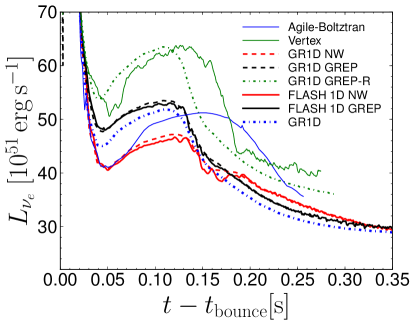
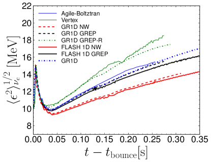
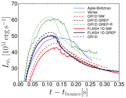
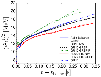
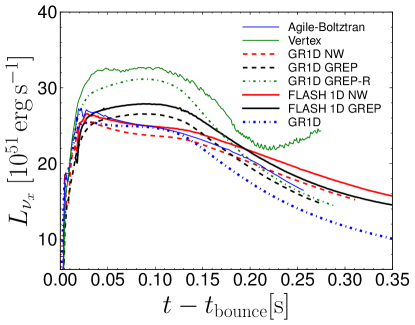
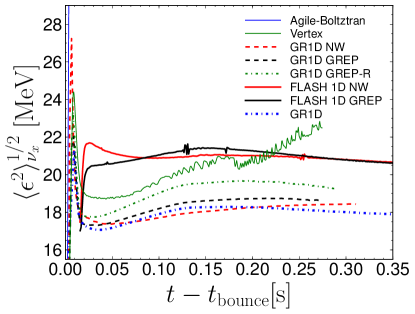
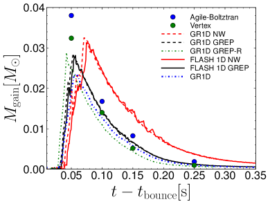
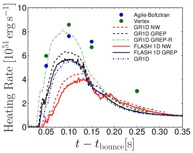
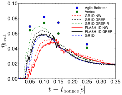
We use the 15 $M_{\odot}$ core-collapse supernova progenitor profile from Woosley & Weaver (1995) as a test case, denoted throughout as s15WW95. To make comparisons with previous publicly available work (Liebendörfer et al., 2005), we use the Lattimer & Swesty EOS with an incompressibility of 180 MeV (LS180; Lattimer & Swesty 1991). For this test only, following Liebendörfer et al. (2005), we do not include weak magnetism and recoil corrections for the neutrino opacities. We present the results in Fig. 1 and Fig. 2. For both figures and in all panels, red lines are collapse calculations using Newtonian gravity, black lines are calculations using our standard general relativistic effective potential, ‘case A’, from Marek et al. (2006). The green lines (thin dashed-dotted) in uses ‘case R’ from Marek et al. (2006) and are presented for comparison purposes with the data extracted from the publicly available Vertex data presented in Liebendörfer et al. (2005). Finally, the blue (thick dashed-dotted) line is from a fully general relativistic calculation using GR1D (data is from O’Connor 2015) while the solid blue line and blue dots are data taken from publicly available Agile-Boltztran data from Liebendörfer et al. (2005). For the red and black lines, the thin dashed lines correspond to data taken from GR1D and the thick dashed lines are from FLASH. We note that all of the GR1D simulations (both GREP and full GR) include inelastic scattering of neutrinos on electrons, while FLASH does not. This aspect is especially important during the collapse phase, hence, we start all FLASH simulations from GR1D profiles at $\sim$15 ms after bounce. For our s15WW95 FLASH simulations the outer extent of our domain is taken to be $10^{9}$ cm.

Fig. 1 shows the fluid-frame neutrino luminosity and root mean squared energy, respectively, of electron neutrinos (top panels), electron antineutrinos (middle panels), and heavy-lepton neutrinos (bottom panels) extracted from the simulations at 500 km. Fig. 2 shows the mass in the gain region (top), the total heating rate in the gain region (middle) and heating efficiency (bottom). The gain region is defined as the region within the shock, but outside the neutrinosphere, where there is an increasing internal energy of the matter due to neutrino interactions. The heating efficiency is defined as the ratio of the rate of energy deposition into the gain region ($\dot{Q}^{\mathrm{gain}}_{\mathrm{heat}}$) to the total electron-type neutrino luminosity at the gain radius. Since the latter is difficult to estimate in multidimensional simulations, we estimate it by adding the heating rate to the lab-frame neutrino luminosity extracted from our simulations,

$$\eta_{\mathrm{heat}}=\frac{\dot{Q}^{\mathrm{gain}}_{\mathrm{heat}}}{L^{\mathrm{lab}}_{\nu_{e}}+L^{\mathrm{lab}}_{\bar{\nu}_{e}}+\dot{Q}^{\mathrm{gain}}_{\mathrm{heat}}}\,.$$ (15)

For the data from Liebendörfer et al. (2005), we project their fluid frame luminosity to the lab frame via $L^{\mathrm{lab}}_{\nu}\sim L^{\mathrm{fluid}}_{\nu}(1+v/c)/(1-v/c)$.

Generally, the deeper gravitational well of the general relativistic simulations (represented by blue, black, and green lines) allows more gravitational binding energy to be released during the accretion phase and results in a higher electron neutrino and electron antineutrino luminosity, which are predominately fueled by accretion, when compared to the Newtonian simulations (red lines). The deeper gravitational well also leads to higher matter temperatures at the neutrinospheres and therefore higher root mean squared energies. This gives larger heating rates and heating efficiencies. The ‘case R’ effective gravitational potential (labeled as GR1D GREP-R; green curve) overestimates the correction to the gravitational potential and gives even higher luminosities and energies (Marek et al., 2006). Important for our discussion is that our ‘case R’ results (green lines) closely match the ‘case R’ results from the Vertex code (Liebendörfer et al., 2005) This agreement, along with the effective potential test cases in Appendix A, gives us confidence in our effective potential implementation. The improved effective potential presented by Marek et al. (2006), (their ‘case A’), comes much closer to reproducing the neutrino luminosities, and matches very closely the root mean squared energies, of the full GR codes Agile-Boltztran and GR1D.

The differences that are seen between the GR1D and GR1D-GREP collapse results are due to the differences between the Newtonian hydrodynamics + GR effective potential gravity and GR hydrodynamics + GR gravity. These differences are also on the order of the differences between the FLASH simulations and the GR1D-GREP simulations, which differ on the hydrodynamics. With the exception of the heavy-lepton neutrino quantities, which are discussed below, the various calculations differ by $\sim 2-5\%$ in the neutrino luminosities and root mean square energies. The differences in the heating related quantities are somewhat larger, $\sim 10\%$, owing to their non-linearly dependence on the neutrino field.

The largest difference between the GR1D and FLASH results is seen in the heavy-lepton sector which is a direct result of the neglect of inelastic neutrino-electron scattering (NES). After bounce, the main effect of NES is to down-scatter neutrinos (Thompson et al., 2003). Electron-type neutrino and antineutrinos have charged-current interactions that keep those neutrinos thermodynamically coupled to the matter until low densities where NES is not as effective. However, heavy-lepton neutrinos, which lack these charged-current interactions, experience a large scattering dominated region where NES plays an important role. The FLASH simulations, both GREP and NW, have on average 4-6 MeV higher ($\sim 25\%$) heavy-lepton $\nu_{x}$ root mean squared energy and $\sim 2\times 10^{51}$ erg s^-1 ($\sim 10\%$) higher luminosities, consistent with the observations of Thompson et al. (2003). However, within the time simulated, the different $\nu_{x}$ luminosities or the additional heating at higher densities supplied by inelastic NES does not have an influence on the electron-type neutrino luminosities or energies, and therefore the heating quantities. For the purposes of neutrino signal prediction, this assumption is quite severe, however there is little effect on the early core-collapse supernova dynamics.

3.2 2D Newtonian Results

Figure 3: Simulation results from 1D and 2D core collapse using Newtonian gravity in four models. We show the time evolution of the mean shock radius (left); $\tau_{\mathrm{adv}}/\tau_{\mathrm{heat}}$ (right). Solid lines are from 2D simulations, while dashed lines are from 1D simulations. To reduce the scatter, we average $\tau_{\mathrm{adv}}/\tau_{\mathrm{heat}}$ over a 5 ms window.

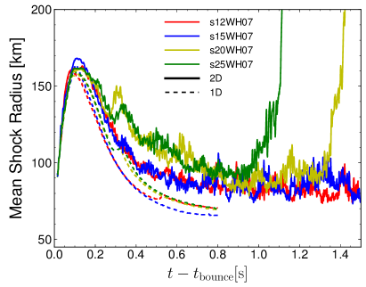
We perform a total of six two-dimensional core collapse simulations using Newtonian gravity. For all simulations, we start from profiles taken from GR1D 15 ms after bounce. We perform four simulations of the models introduced in Table 1, s12, s15, s20, and s25 from Woosley & Heger (2007) (WH07). We use our base resolution and the LS220 EOS. As mentioned in §2.1, we assume $l_{\mathrm{max}}=0$ in our multipole gravity solver. We have tested this assumption by performing a Newtonian transport simulation with model s12 and with $l_{\mathrm{max}}=24$. Finally, we test our effective potential solver by performing a Newtonian simulation with the s12 progenitor and where the gravity is computed via the algorithm in §2.1, but replacing the differential equations with the Newtonian equivalents. Theoretically, this is precisely the same as the standard monopole term for the gravity, but numerically calculated in a different way. For both of these latter two test simulations we see no differences other than the stochastic behavior of the convection and turbulence.

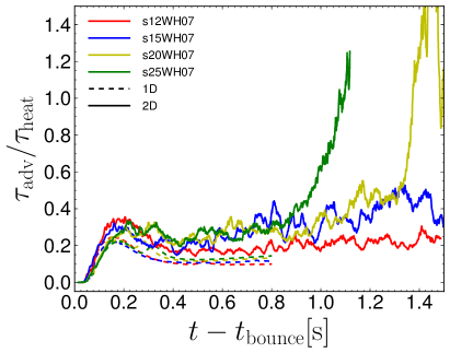
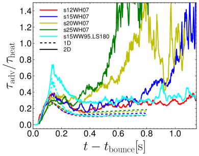
In Fig. 3, we show a subset of results from our Newtonian simulations. We see a very late time ($\gtrsim 1\,$s) explosion in two models, s20 and s25, and failure in the other models, s12 and s15. Other than the late time explosion, the simulations of the four models proceed similarly. In both 1D and 2D, in all four models, the shock initially expands out and reaches $\sim$160-170 km at $\sim$100 ms after bounce. Only at this time do the 1D and 2D simulations begin to depart from each other as convection begins to strongly develop behind the shock and provide additional pressure support for the supernova shock (Murphy et al., 2013; Couch & Ott, 2015). In 1D and 2D the shocks begin to recede. Compositional interfaces reach the shock front at $\sim$250 ms, $\sim$300 ms, and $\sim$500 ms for models s20, s25, and s12, respectively. At these times, especially in models s25 and s20, we see a short phase of shock expansion. The shock expansion is more prominent in 2D than in 1D. However, this is not sufficient to reenergize the shock in these simulations. At late times the accretion rate has dropped enough to drive an explosion. However, we caution that at these times the baryonic mass of the PNSs is approaching 2.2 $M_{\odot}$. The Newtonian gravity approximation is expected to be far from valid in this regime as the maximum baryonic mass of the LS220 EOS $2.41\,M_{\odot}$.

A useful diagnostic of proximity to explosion is the ratio of the advection time through the gain region to the time it takes to unbind the gain material through neutrino heating. A ratio of 1 can be thought of as a runaway condition where matter is unbound before it can be advected into the cooling region. Quantitatively we define this ratio via,

$$\frac{\tau_{\mathrm{adv}}}{\tau_{\mathrm{heat}}}=\frac{M_{\mathrm{gain}}/\dot{M}}{|E_{\mathrm{gain}}|/\dot{Q}_{\mathrm{heat}}}\,.$$ (16)

We define the gain region to consist of any grid zone with a net positive change in the internal energy of the matter due to neutrino interactions. $M_{\mathrm{gain}}$ is the total mass of those grid zones, $\dot{M}$ is the accretion rate measured at 500 km, $\dot{Q}_{\mathrm{heat}}$ is the rate of energy exchange between the neutrino and the matter in the gain region, and $E_{\mathrm{gain}}=\sum_{\mathrm{gain}}m_{i}[1/2|v_{i}|^{2}+\epsilon_{i}+\phi_{i}]$ , is the energy of the matter in the gain region. For the latter, $v_{i}$ is the matter velocity, $\phi_{i}$ is the gravitational potential, and $\epsilon_{i}$ is the specific internal energy of the matter. For consistency with other works, we take the zero point defined in LS220 EOS for $\epsilon_{i}$. In the top right panel of Fig. 3 we show this quantity for our Newtonian models. For most of the time, the WH07 models we simulate are well below $\tau_{\mathrm{adv}}/\tau_{\mathrm{heat}}\sim 1$. Only at late times does this ratio approach 1 for the two exploding models.

Figure 4: Simulation results from 1D and 2D core collapse using GR effective gravity in five models. We show the time evolution of the mean shock radius (top and middle) and $\tau_{\mathrm{adv}}/\tau_{\mathrm{heat}}$ (bottom). Solid lines are from 2D simulations, while dashed lines are from 1D simulations. Models s12, s15, s20, and s25 are performed with the LS220 EOS, model s15WW95 uses the LS180 EOS for comparison purposes. To reduce the scatter, we average $\tau_{\mathrm{adv}}/\tau_{\mathrm{heat}}$ over a 5 ms window.

Figure 5: Neutrino quantity results from 1D and 2D core collapse using GR effective gravity in five models. We show the time evolution of the $\nu_{e}$ (top), $\bar{\nu}_{e}$ (middle), and $\nu_{x}$ (bottom) luminosity (left) and root mean squared energy (right). Solid lines are from 2D simulations, while dashed lines are from 1D simulations. Models s12, s15, s20, and s25 are performed with the LS220 EOS, model s15WW95 uses the LS180 EOS for comparison purposes.

3.3 2D Effective GR Results

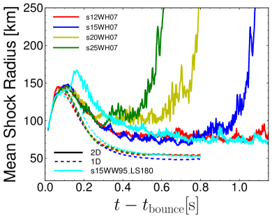
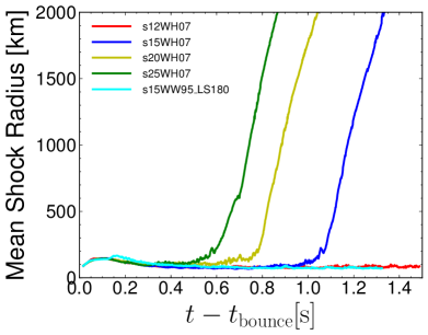
In our simulations using the GR effective potential we achieve runaway supernova shocks in our core collapse simulations for three of the four progenitors models: s15, s20, and s25. These explosions occur at significantly earlier times compared to the Newtonian simulations. We attribute this to the increased heating in the GREP simulations discussed in the context of 1D models presented in §3.1. This increased heating is a result of the more compact PNS configurations afforded by GR gravity. This gives higher electron neutrino and antineutrino luminosities and root mean squared energies. In Fig. 4, we show the evolution of the mean shock radius in our GREP simulations. The top panel shows the early shock development, while the middle panel shows the shock evolution out to 2000 km. The WH07 simulations start very similar to the pure Newtonian simulations. Initially, the shock radius extends out to $\sim$145 km at $\sim$100 ms, roughly 15 km lower than the Newtonian simulations. As with the Newtonian simulations, the shock begins to recede in both 1D and 2D. By the end of the simulated time, we achieve explosions in three of the four models. The times at which the mean shock radii reach 500 km are $\sim$1100 ms, $\sim$820 ms, and $\sim$670 ms for models s15, s20, and s25, respectively. These values are listed in Table 1. The s15WW95_LS180 model is markedly different than the WH07 models, the shock radius stagnates at a slightly lower radius, $\sim$140 km, then extends to a much larger radius ($\sim$170 km) after the compositional interface accretes through the shock at $\sim$150 ms before ultimately receding and failing to be reenergized.

In the bottom panel of Fig. 4, we show the ratio of the advection time through the gain region to the time it takes to unbind the matter in the gain region due to neutrino heating, $\tau_{\mathrm{adv}}/\tau_{\mathrm{heat}}$, defined in Eq. 16. In models s15, s20, and s25, $\tau_{\mathrm{adv}}/\tau_{\mathrm{heat}}$ surpasses unity at $\sim$1 s, $\sim$700 ms, and $\sim$560 ms, which corresponds to the time when the mean shock radius is starting its outward propagation. The s12 and s15WW95_LS180 models never surpass the value of unity, these models do not explode. For the exploding models, large, late-time asymmetries in the explosion morphology lead to values of $\tau_{\mathrm{adv}}/\tau_{\mathrm{heat}}$ less than unity. This is due to the break down of the underlying assumptions of Eq. 16, which is technically only valid for spherical flows.

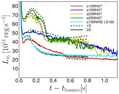
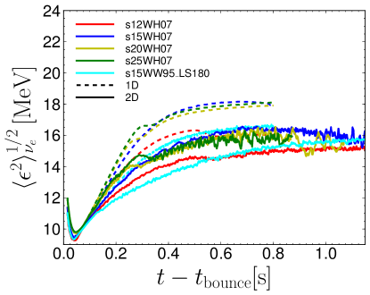
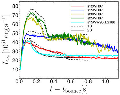
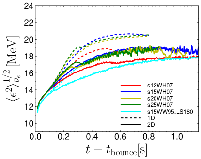
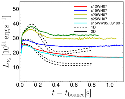
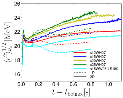
The left column of Fig. 5 shows the luminosity of each of the three neutrino species. Prior to explosion, or for the entire evolution for models s12 and s15WW95_LS180, the neutrino luminosities closely follow the 1D simulation. This is because the neutrino luminosity being emitted in simulations with stalled or failing supernova shocks is set by the accretion rate, which is the same in both 1D and 2D. The situation changes after the explosion sets in. After this time, not all accreted matter is able to settle into the cooling region since it is being heated by neutrinos and unbound. As a result, the released gravitational binding energy is not being converted into neutrino luminosity. The consequence is that the post-explosion neutrino luminosity in 2D is lower than the neutrino luminosity determined in the 1D simulation at the same time. Our $\nu_{x}$ luminosities are not as dramatically influenced by the fluid motions in the gain region as they are emitted from deeper in the cooling region away from the convective motions. Consequently, they show less variability than both $\nu_{e}$ and $\bar{\nu}_{e}$. However, there is a significant multidimensional effect on the $\nu_{x}$ neutrinos. We see a boost in the $\nu_{x}$ luminosities due to PNS convection. This convection slows the recession of the neutrinosphere, and dredges up heat from deeper in the PNS. This results in an increase in the $\nu_{x}$ luminosity and $\nu_{x}$ root mean squared energy (right column of Fig. 5) starting around $\sim$200 ms. It is also responsible for lowering the electron type neutrino and antineutrino root mean square energies. We give a more detailed discussion of PNS convection in §4.

Figure 6: Diagnostic explosion energies for exploding models determined via Eq. 17 (top panel) and cumulative PNS baryonic mass (bottom panel). The explosion energy estimate includes an estimate of the nuclear recombination energy, but does not include the binding energy of the overlying star. We also show (dashed and dashed-dotted lines) tests with the s25 model where we decrease the resolution and where we decreased the resolution but increase the number of neutrino energy bins. For the bottom panel, the PNS is defined as the region with matter densities larger than $10^{11}$ g cm^-3. Solid lines denote the mass from 2D simulations while dashed lines show the PNS mass from 1D simulations.

Figure 7: Entropy color plots of exploding models s15, s20, and s25 at 1340 ms, 1070 ms, and 830 ms after bounce, respectively. These times correspond to when the shock front first reaches 4000 km. The explosions are strongly asymmetric, indicative of weak explosions. Grey zones correspond to the shock position and blue $\to$ green $\to$ yellow $\to$ orange $\to$ red colors denote increasing values of the entropy

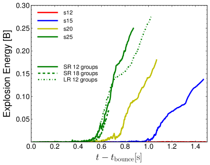
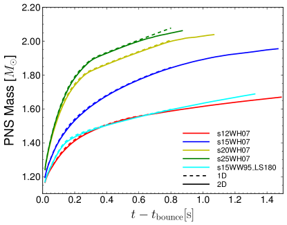
In the top panel of Fig. 6, we show the early development of the diagnostic explosion energy (Buras et al., 2006b; Bruenn et al., 2013; Melson et al., 2015),

$$E_{\mathrm{exp}}^{\mathrm{diag}}=\int_{\mathcal{V}}d\mathcal{V}\rho[1/2|v|^{2}+(\epsilon-\epsilon_{0})+\phi]_{>0}\,,$$ (17)

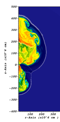
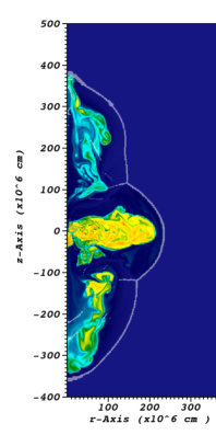
where the volume integral is over all zones where the integrand is positive. $\phi$ is the gravitational potential energy, $\epsilon$ is the specific internal energy and $\epsilon_{0}$ is the specific internal energy of matter with the same density and $Y_{e}$, but $T=0$. This roughly accounts for the energy that will be released into kinetic energy as the matter cools and the free nucleons recombine into alpha particles, and later nuclei. To truly determine this energy, one must track the evolution to much longer times and do a proper treatment of nucleosynthesis, something we are not capable of doing with our current infrastructure. We also note that this diagnostic explosion energy does not account for the binding energy of the material outside the shock (i.e, the “overburden”) which can be significant in the higher mass models, perhaps upwards of 1 B (Bruenn et al., 2016). Our explosion energies are quite small compared to the results of Bruenn et al. (2013), and more along the lines predicted from other successful explosions in two and three dimensions (Hanke et al., 2012; Melson et al., 2015; Müller et al., 2012b; Suwa et al., 2010; Pan et al., 2016; Suwa et al., 2016). We do note that the amount of simulated post-explosion time is short. In our simulations, along with the weak explosions comes continued accretion after the explosion sets in. We show this in the bottom panel of Fig. 6, where we show the PNS mass (PNS defined as the region with a matter density of at least $10^{11}$ g cm^-3) in 2D (solid lines) and 1D (dashed lines). The simulations which do not produce explosions have similar PNS masses in 1D and 2D. For the simulations that explode, the growth of the PNS mass slows after the explosion sets in, but is not zero in any model at the latest times simulated. Finally, we note that the explosions are highly non-spherical with strong accretion occurring along various directions. We show graphical snapshots of our three exploding models in Fig. 7 at a time determined by when the maximum shock radius reaches 4000 km, corresponding to 1340 ms, 1070 ms, and 830 ms after bounce for models s15, s20, and s25, respectively.

3.3.1 Resolution and Random Perturbations

We simulate core collapse in model s25 with a lower resolution. As discussed in § 2.3, our production simulations have a central cell size of $\sim$488 m and maintain an effective angular ($\Delta r/r$) resolution from at least 0.5 degrees outside $\sim$55 km. This results in the first refinement decrement (from $\sim$500m to $\sim$1 km) at $\sim$107 km. For our lower resolution simulation, we only enforce an effective resolution of 0.9 degrees, giving refinement decrements at $\sim$65 km, $\sim$139 km, and so on. In addition to this simulation we also simulate model s25 at our standard resolution and with 18 energy groups instead of our standard 12. In both tests, explosions develop at similar times to our baseline model. The development of the explosion energies for the successful models (see dashed and dashed-dotted lines in Fig. 6) are similar between these tests.

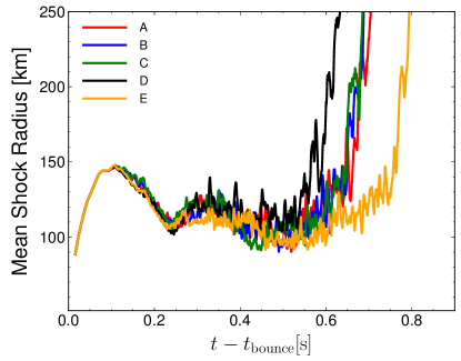
As a further test, we explore the effect of imposed random perturbations on the development of the explosion. We simulate model s20 five times, each time perturbing the initial density field (when we transition from our 1D model to the 2D simulations at $\sim$15 ms after bounce) randomly (and uniformly) by up to $\pm 0.1\%$. We show the evolution of the shock radii in Fig. 8. Stochastic variations in the hydrodynamic instabilities behind the shock cause the explosion times (determined by when the mean shock passes 400km) to vary from $\sim$670 ms to $\sim$830 ms. The average is $\sim$723 ms with a formal variance of $\sim$63 ms. We note that the explosion time of our main simulation of s20 falls near the latter end of this range. These simulations are also discussed in O’Connor et al. (2017).

Figure 8: Shock radius evolution for five simulations of model s20, each started with different random density perturbations. The explosion times differ due to stochastic variations in the postshock region.

4 Discussion

4.1 GR vs Newtonian Gravity

Figure 9: Neutrino heating metrics for 2D simulations with both GR effective potential gravity and Newtonian gravity. We show the net heating (top panel), the heating efficiency (middle panel), and non-radial kinetic energies in the gain region (bottom panel) for each of the four WH07 models and model s15WW95_LS180 used in this study. Simulations with Newtonian gravity are shown as dashed lines while the GR effective potential simulations are solid lines. For the bottom panel, models s20 and s25 are shifted up for clarity. All curves are averaged over 5ms to reduce noise.

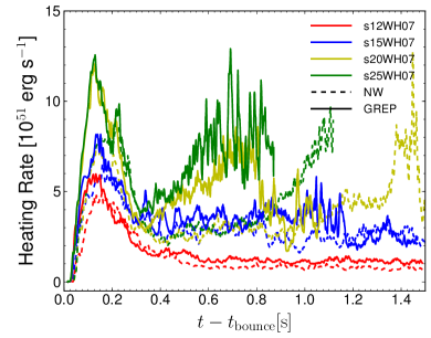
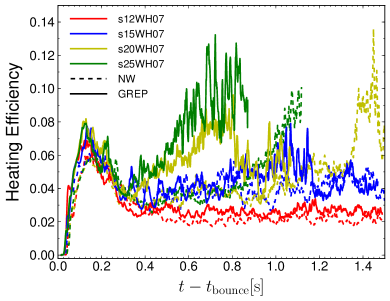
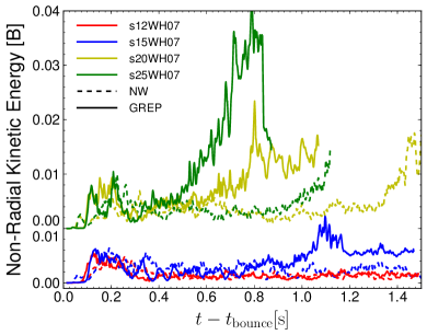
From the results presented in the last section, it is clear that the approximation of Newtonian gravity gives less favorable conditions for a successful core-collapse supernova explosion than the more realistic GR treatment. Even though we do not include full GR gravity and hydrodynamics, the test results of §3.1, and the comparisons to the previous work of Liebendörfer et al. (2005); Marek et al. (2006); O’Connor (2015) convince us that using an effective GR potential allows us to capture the important aspects of GR for modeling core-collapse supernovae. Most importantly, the 1D results of §3.1 show that GR gravity leads to higher neutrino luminosities, and higher root mean squared energies which directly follow from a more compact PNS structure. The neutrino mechanism relies on the capture of neutrinos emitted from the cooling region into the gain region. This capture is greater with higher luminosities, and more efficient with higher neutrino energies. However, in 1D, the added benefits of GR do not lead to successful explosions as has been previously demonstrated (Liebendörfer et al., 2001). This trend of increased heating and higher heating efficiencies carries over to 2D, which we demonstrate in Fig. 9. In this figure, we show the net heating rate in the gain region (top), the heating efficiency (middle; Eq. 15), and the non-radial kinetic energy in the gain region (bottom) for the four WH07 models using the GR effective potential gravity (solid lines) and Newtonian gravity (dashed lines). In all models, both the heating rate and the heating efficiency are larger in the simulations using the GR effective potential, by up to $\sim$20-30% between 100 ms and 200 ms after bounce. Furthermore, the appearance of the gain region occurs sooner for the GREP models by $\sim$20 ms. We also generally see more non-radial kinetic energy in the gain region, which is a sign of stronger neutrino-driven convection. As a consequence of these improved neutrino heating conditions, we see earlier explosions in the GREP models s20 and s25 by $\sim$0.5 s and an explosion in the GREP model s15 where the Newtonian model did not explode.

4.2 Comparison to Literature

4.2.1 Newtonian Gravity

In Table 1 we have summarized other studies in the literature which simulate the four models simulated here and use Newtonian gravity. They include Dolence et al. (2015); Suwa et al. (2016); Pan et al. (2016). Many aspects of our results compare quite well to the Newtonian results of Dolence et al. (2015). Dolence et al. (2015) use the same progenitor models, the same neutrino microphysics (based on Bruenn 1985; Burrows et al. 2006), and also a truly multidimensional neutrino transport scheme, albeit MGFLD. Matching our simulations, none of the 2D simulations in Dolence et al. (2015) explode before 600 ms, which is when their simulations stop. Comparison of $\tau_{\mathrm{adv}}/\tau_{\mathrm{heat}}$ show good agreement. At $\sim$200 ms, $\tau_{\mathrm{adv}}/\tau_{\mathrm{heat}}\sim 0.3-0.4$ in both simulation sets and for all four models. Furthermore, our heating efficiencies (see Fig. 9) near $\sim$200 ms after bounce are $\sim$0.06, similar to the values of $\sim$0.065-$\sim$0.085 seen by Dolence et al. (2015). Two-dimensional Newtonian simulations of these models are also presented in Suwa et al. (2016) using IDSA for neutrino transport. There, the LS220 EOS is used. They observe an early explosion in a few models, including s12, and failure in the majority of the rest. One issue preventing a detailed comparison is that Suwa et al. (2016) ignore heavy-lepton neutrinos in their simulations. It is likely the case that this prevents the PNS from cooling and causes the shock to initially stall at $\sim 240$ km and hover around $\sim$200 km in failed models. Pan et al. (2016) also perform Newtonian axisymmetric simulations of core collapse using IDSA for neutrino transport. However, they find early explosions for all progenitors simulated: 11 M_⊙, 15 M_⊙, 21 M_⊙, and 27 M_⊙ models from Woosley et al. (2002) as well as two of the models explored here: s15 and s20. It is worth noting that later simulations in Pan et al. (2017) find no explosions in models s15 and s20 with Newtonian gravity.

4.2.2 GR Gravity

We also compare to studies in the literature that use GREP gravity. These include Summa et al. (2016); Bruenn et al. (2016). We will first discuss the results of Summa et al. (2016). Summa et al. (2016) achieve explosions in all four models studied here. Their explosion times are $\sim$790 ms, $\sim$620 ms, $\sim$320 ms and $\sim$400 ms for models s12, s15, s20, and s25, respectively. These explosions times are earlier than ours by $\sim$300-$\sim$500 ms. We do not see an explosion in model s12 before $\sim$1.5 s, when our simulation was stopped. The evolution of the mean shock radius is qualitatively similar. The initial stalling radius in our simulations is $\sim$150 km compared to $\sim$160 km in Summa et al. (2016). After this, there is a period of shock recession before the ultimate shock expansion. However, the simulations of Summa et al. (2016) have a much more pronounced shock recession. This may stem from the differences in the neutrino interactions used. Summa et al. (2016) use inelastic neutrino-nucleon scattering and absorption opacities from Burrows & Sawyer (1998, 1999) whereas we use simpler elastic rates from Bruenn (1985). They use microphysical electron capture rates on heavy nuclei for the collapse phase instead of the approximate form from Bruenn (1985) implemented here. Finally, Summa et al. (2016) include neutrino-neutrino pair scattering and annihilation (to other neutrino pairs) as additional pair-processes. One important consequence of these improved opacities is the more efficient cooling of the PNS which gives higher $\nu_{x}$ luminosities and faster contraction and as a consequence. In O’Connor et al. (2017), we have made the first steps to improve our neutrino interactions by including a correction factor of the neutral-current scattering cross sections that mimics Burrows & Sawyer (1998, 1999). There we found earlier explosion times by $\sim$100-150 ms. Given these lingering differences between our simulations and those of Summa et al. (2016), a comparison with even closer underlying physics is warranted. Although we find it quite encouraging that we find relatively close agreement on many quantities, including neutrino luminosities, neutrino energies, neutrino heating rates and efficiencies, and explosion diagnostics like $\tau_{\mathrm{adv}}/\tau_{\mathrm{heat}}$, even with the differences between our simulation codes and simulation techniques.

In contrast, our results are in qualitative disagreement with the results of Bruenn et al. (2013, 2016) (labeled here as Bruenn et al.). At 100 ms, all four models in Bruenn et al. stall at a radius of $\sim$200 km. However, after the shock stalls it continues to slowly move out in radius until it ultimately begins to run away. There is no period of shock recession in any model. We note, however, an updated 2D simulation in Lentz et al. (2015) of model s15 gives a stall radius of $\sim$175 km, there is still no recession of the shock front in this updated simulation. We can also directly compare neutrino quantities and heating rates with the results in Bruenn et al. The neutrino luminosities predicted from both sets of simulations agree within $\sim$5% (this difference is in part due to the fact that Bruenn et al. measure their quantities in the co-moving frame at 1000 km where the fluid velocities are $\sim 0.03\,c$). The root mean squared energies (right column of Fig. 5) show a larger difference, Bruenn et al. predict neutrino energies up to $\sim 20\%$ larger than our results at $\sim$100 ms after bounce, this difference cannot be explained by the difference between the co-moving frame measurements alone, but could be due to differences in the neutrino interactions (which include some of the improved rates included in Summa et al. (2016) listed above, but not the neutrino-neutrino scattering or annihilation to other neutrino pairs) or the neutrino transport (which is MGFLD, a more approximate, one moment transport scheme using the ray-by-ray+ approximation). Roughly, the neutrino heating rates scale with both the electron-type neutrino luminosity and the electron-type mean squared neutrino energy, therefore we expect to see the influence of the higher root mean squared energies seen in Bruenn et al. reflected in the heating rates. Our GREP simulations have a net heating rate in the gain region at 100 ms after bounce of $\sim$6 B $s^{-1}$, $\sim$6 B $s^{-1}$ $\sim$10 B $s^{-1}$, and $\sim$10 B $s^{-1}$ for models s12, s15, s20, and s25, respectively, while the heating rate in Bruenn et al. at the same time are $\sim$9 B $s^{-1}$, $\sim$13 B $s^{-1}$, $\sim$20 B $s^{-1}$, and $\sim$20 B $s^{-1}$, for models s12, s15, s20, and s25, respectively (the heating rate at 100 ms after bounce in the updated 2D simulation of model s15 in Lentz et al. (2015) is 9 B s^-1). The heating rates seen in the Bruenn et al. simulations are roughly $\sim$50% higher than ours. This large discrepancy at such an early postbounce time warrants further investigation beyond comparison of literature results.

4.2.3 1D Parameterized Models

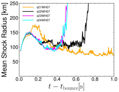
We note that the heating efficiency of successful models is significantly less than the heating efficiency one would predict was required for an explosion in 1D. For example, O’Connor & Ott (2011) predicts a critical heating efficiency of 0.172, 0.176, and 0.185 for models s15, s20, and s25. The success of these models in our simulations is not due solely to the increase in neutrino heating as a result of multidimensional instabilities, rather the instabilities themselves are directly contributing to success of the explosion (Couch & Ott, 2015). Our results, while only consisting of four models, are inconsistent with the 1D parameterized model predictions of success/failure from Ertl et al. (2016): our exploding models are predicted to fail and our failed model is predicted to succeed. To extend this further we have simulated four additional models, s21, s22, s23, and s24 from Woosley & Heger (2007). Based on Ertl et al. (2016), s21 is predicted to explode and the remaining models are predicted to fail. In particular, models s22 through s25 are in a region of ZAMS mass that many studies have predicted will from failed supernovae and black holes. As can be seen in Fig. 10, this is not the case, similar to the pattern observed in the other models, the s21 model fails to explode while the other three models successfully explode. We note the similarity of the shock evolution in s21 to that of s15WW95. These two models have remarkably similar presupernova structure in the inner regions, characterized by a steep gradient in the density at a compositional interface at relatively low mass coordinate (compared to the other models explored here). The ultimate predictive power of 1D parameterized explosion models like these must be further tested (or calibrated) with multidimensional models, preferably three dimensional models. The impact of the multidimensional dynamics on the explosion mechanism is likely significant enough that modeling it through increased neutrino heating alone may not be sufficient.

Figure 10: Shock radius evolution for four simulations of models s21, s22, s23, and s24. All models except s21 explode, contrary to predictions based on 1D parameterized models.

4.3 Impact of Protoneutron Star Convection

Figure 11: Color maps of the Brunt-Väisälä frequency (left, center) from the 1D and 2D GREP s20 simulations as a function of time and radius. Red colors denote convectively unstable regions while blue regions are convectively stable. The right panel shows the anisotropic velocity of the 2D model. Shown as green, magenta, and red lines are the mean shock radius, maximum shock radius, and gain radius, respectively. We mask out the color map above the mean shock radius. In the right panel, the black and grey lines show the 2D and 1D, respectively, heavy lepton neutrinosphere.

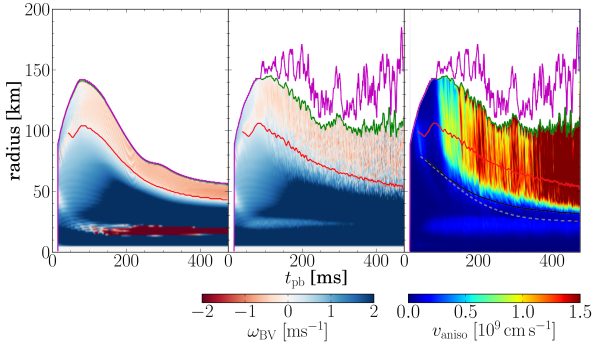
Our 2D models develop PNS convection starting at $\sim$60 ms after bounce. As mentioned earlier, this convection has a quantitative impact on the neutrino luminosities, particularly the heavy lepton neutrino luminosities. We will discuss PNS convection in more detail here.

In Fig. 11, we show color maps of the Brunt-Väisälä frequency, $\omega_{\mathrm{BV}}$, as a function of time and radius for the GREP model s20, for both 1D (left) and 2D (center). While convection will not develop in our 1D model, examining $\omega_{\mathrm{BV}}$ is useful nonetheless. For each time slice (angle averaging the matter properties in the case of 2D) we compute $\omega^{2}_{\mathrm{BV}}$ (Foglizzo et al., 2006),

$$\omega^{2}_{\mathrm{BV}}=\frac{d\phi}{dr}\left(\frac{1}{\gamma}\frac{d\ln{P}}{dr}-\frac{d\ln{\rho}}{dr}\right)\,,$$ (18)

and take

$$\omega_{\mathrm{BV}}=\mathrm{sign}(\omega^{2}_{\mathrm{BV}})\sqrt{|\omega^{2}_{\mathrm{BV}}|}\,,$$ (19)

where $d\phi/dr$ is the radial gradient of the gravitational potential and $\gamma$ is the adiabatic index. Positive values of $\omega_{\mathrm{BV}}$ (blue) denote convectively stable regions while negative values (red) denote convectively unstable regions. On each graph we also show the mean and maximum shock radius as green and magenta lines, respectively, and the average gain radius as a red line. While the Brunt-Väisälä frequency shows the susceptibility to convection, the anisotropic velocity,

$$v_{\mathrm{aniso}}=\sqrt{\frac{\langle\rho[(v_{r}-\langle v_{r}\rangle)^{2}+v_{\theta}^{2}]\rangle}{\langle\rho\rangle}}\,,$$ (20)

shows the actual presence of convective motions. The right panel of Fig. 11 show the anisotropic velocity in the 2D simulation of s20. Also in this panel we show the location of the heavy-lepton neutrinosphere from the 1D simulation (dashed line) and from the 2D simulation (solid line). The neutrinosphere is defined as the location where the spectrum weighted flux factor equals 0.25. We note several important results from these graphs below.

Before discussing PNS convection in detail, we will briefly discuss the development of convection in the gain region. The 1D and 2D maps of $\omega^{2}_{\mathrm{BV}}$ are very similar up to $\sim$100 ms after bounce. Even though there is a convectively unstable region close to the shock front, due to the high advection rate of material through this region convective seeds are unable to grow to full scale convection before the matter is accreted out of the unstable region. By $\sim$100 ms the accretion rate has dropped, the shock radius increased, and the convectively unstable region has grown so that convective motions begin to develop in earnest as seen through the rise of $v_{\mathrm{vaniso}}$. This causes the shock radius to deviated from the spherically symmetric solution at this time. The added pressure support to the material behind the shock from these anisotropic motions is crucial to aid the neutrino mechanism and help drive an explosion (Couch & Ott, 2015; Müller & Janka, 2015).

Fig. 11 also shows the development of a region that is unstable to PNS convection between $\sim$15 km-$\sim$25 km starting as soon as $\sim$60 ms after bounce in the 1D model. While we just show the GREP model s20, such a region is present in all models. In the corresponding 2D simulation, the onset of PNS convection occurs at this time, as seen in the color map of $v_{\mathrm{aniso}}$, and works to maintain $\omega^{2}_{\mathrm{BV}}\sim 0$. This convection has a quantitative effect on the neutrinos being emitted in our 2D simulations. PNS convection effectively transfers internal energy from deep in the PNS to slightly larger radii. This helps support the PNS and prevents the neutrinospheres from receding as they do in the corresponding 1D simulations. This predominantly impacts the heavy-lepton neutrinos as they are emitted from the deepest regions of the star, closest to the PNS convection zone. We explicitly show the heavy lepton neutrinosphere location in the right panel of Fig. 11, the solid line is the neutrinosphere from the 2D simulations while the dashed line is from the corresponding 1D simulation. The increased neutrinosphere radius, and the higher matter temperatures at the typical radius where the heavy lepton neutrinos are emitted from gives a larger $\nu_{x}$ luminosity as can be seen in Fig. 5. We note that increases, which have also been attributed to PNS convection, in the $\nu_{x}$ luminosities are seen in 1D vs. 2D models as early as Buras et al. (2006a) and more recently in Radice et al. (2017). However, it is worth mentioning that Buras et al. (2006a) see a relatively smaller impact of PNS convection on the heavy-lepton neutrino luminosity (an increase of, at most, $\sim 20\%$) than seen here or in Radice et al. (2017).

5 Conclusion

The study of core-collapse supernovae is an exceedingly multi-physics problem. If anything, decades of research into the core-collapse supernova central engine has shown that in order to create realistic simulations of these astrophysical phenomena we need to include all of the important underlying physics. This includes, but is of course not limited to, the nuclear equation of state, neutrino transport and neutrino interactions, general relativistic gravity, realistic progenitor models, resolved multidimensional (3D) magnetohydrodynamics, and more. In this paper, we have extended the capabilities of the FLASH simulation package to now include an effective treatment of general relativistic gravity and a multispecies, multigroup, multidimensional, velocity-dependent neutrino-radiation transport solver. Both of these new implementations are designed for application to the core-collapse supernova problem.

We have tested our GR implementation of gravity and our neutrino transport solver with several classic test problems, including an unstable TOV migration test (in both 1D and 2D), and the M1 shadow test. Furthermore, we perform the benchmark core-collapse test case for GR neutrino radiation transport + hydrodynamics from Liebendörfer et al. (2005) which uses a base set of neutrino interactions based on Bruenn (1985), the LS180 nuclear EOS from Lattimer & Swesty (1991), and the 15$M_{\odot}$ progenitor from Woosley & Weaver (1995). Our results closely match those of other neutrino transport methods. We critically assess and make clear the impact of the approximations in our neutrino transport scheme with this comparison.

Extending our simulations to axisymmetry, we study core collapse in four progenitors from Woosley & Heger (2007) with both Newtonian and GR gravity for at least $\sim$800 ms after bounce. While the benefits that a general relativistic treatment of gravity can have for the core-collapse supernova problem have been discussed before, ours is the first study to systematically explore the differences between Newtonian and GR gravity in multiple dimensions and across several updated progenitor models. Our results clearly and unambiguously show that GR gravity significantly aids the neutrino mechanism in reenergizing the stalled supernova shock formed in the core collapse of massive stars. We obtain explosions in three of four progenitor models from Woosley & Heger (2007) when using general relativistic gravity. Two of the four corresponding Newtonian simulations also achieve explosions, however they are delayed by an additional $\sim$500 ms. There are numerous examples in the literature of complicated multi-physics simulations of core-collapse supernova with sophisticated neutrino treatments but only Newtonian gravity. The results presented here show that the approximation of Newtonian gravity can be quite detrimental in the context of core-collapse supernova explosions and should be relaxed if accurate results are sought.

We have also showed the stochastic nature of the core collapse problem in 2D axisymmetry by simulating one model with 5 different sets of random initial perturbations. For this model, we find the explosion time can vary by $\pm\sim$100 ms. Such stochastic variations must be considered when making detailed comparisons between simulations. We have also added four additional models to our GREP simulations, s21, s22, s23, and s24 from Woosley & Heger (2007). This region is predicted from several 1D parameterized explosions studies to be susceptible to black hole formation. We do not see any evidence of this, instead we find explosions in three of four of these models.

Our results match, in several ways, other multidimensional, energy-dependent neutrino radiation transport simulations of core-collapse supernovae including the Newtonian gravity simulations of Dolence et al. (2015) and the GR gravity simulations of Summa et al. (2016). However, differences still exist between the results of these works and the work presented here. This could be due to differences in the neutrino and nuclear microphysics, neutrino transport methods, and/or numerical setups. We find qualitative differences between our work and the work of Bruenn et al. (2013, 2016), which again, could be due to any of the potential differences listed above. We note specifically significant differences in the amount of the neutrino heating present during the early postbounce phase. A close comparison of methods, input physics, and results is warranted to resolve these differences.

Appendix A Neutron Star Migration Test

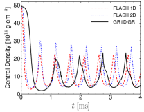
In Fig. 12, we test our GR effective potential implementation via a Tolman-Oppenheimer-Volkoff (TOV) star migration test. We follow the initial conditions from Marek et al. (2006). Our unstable TOV stars follow a $\Gamma=2$ polytropic EOS, $P=K\rho^{\Gamma}$ with a value of $K=1.455\times 10^{5}$ [cgs]. We take an initial central density of $\rho_{c}=4.93\times 10^{15}$ g cm^-3 and solve the ‘case A’ modified TOV equations to obtain the equilibrium (but unstable) structure. With simulate 4 ms of evolution in FLASH, in both 1D (red dashed line) and 2D (blue dashed-dotted). We also use the full GR code GR1D to perform the migration test (black solid line). For this full GR test, we use the standard TOV equations to construct the initial profile. In the effective potential tests, the unstable star quickly ($\sim$0.1 ms) starts its migration away from the unstable configuration, and oscillates about the stable configuration. The full GR evolution is slower, especially at the beginning, which we can understand from the time dilation effect in the full GR simulation, the value of the central lapse for this configuration begins at $\sim$0.27, and migrates to $\sim$0.65. Our results compare very well to the ‘case A’ results and the full GR CoCoNut results of Marek et al. (2006), completing between 7 and 8 oscillation cycles in the first 4 ms of evolution for the effective potentials and $\sim$5 cycles in the full GR case. This convinces us that we have correctly implemented the GR effective potential in both 1D and 2D in FLASH. We have also tested stable TOV star configurations. Using a stable TOV star, with the same EOS and an initial central density of $7.5\times 10^{14}$ g cm^-3, FLASH maintains this central density over 4 ms to better than 1% in 1D and 0.5% in 2D.

Figure 12: Unstable TOV star migration test. This TOV star migration test is performed in FLASH to test our implementation of the ‘case A’ GR effective potential from Marek et al. (2006). We present results from a 1D simulation (red dashed line) a 2D simulation (blue dashed-dotted line) and a full GR simulation in GR1D (black solid line). The results compare quite well to those of Marek et al. (2006) and convince us of the correctness of our effective potential implementation.

Appendix B Neutrino Transport Methods & Implementation

In this appendix we present the details of the numerical techniques used to solve the neutrino transport equations (Eq. 7 to Eq. 11), the microphysics used to compute the neutrino interaction coefficients, and the couple to the hydrodynamics.

Closure: To close the hierarchy of moment evolution equations after the first two moments, we must specify a closure relation for the Eddington tensor $P^{ij}$ in terms of the two lower moments $E$ and $F^{i}$. We choose the common M1 closure and perform the calculation in the fluid rest frame in order to achieve the appropriate limiting cases. Our framework follows closely that of O’Connor (2015); Shibata et al. (2011). In the optically thick regime the radiation in the fluid rest frame is isotropic. For this limit, we write the Eddington tensor as $K^{ij}\equiv K_{\mathrm{thick}}^{ij}=J/3h^{ij}$, where $h^{ij}=1+W^{2}v^{i}v^{j}$ is the projection tensor. In optically thin, free streaming regions far from the source $K^{ij}\equiv K_{\mathrm{thin}}^{ij}=J(H^{i}H^{j}/H^{2})$. For the total Eddington tensor in the fluid rest frame we interpolate between these two limiting regimes,

$$K^{ij}=\frac{3(1-\chi)}{2}K_{\mathrm{thick}}^{ij}+\frac{3\chi-1}{2}K_{\mathrm{thin}}^{ij}\,.$$ (B1)

In these equations $\chi$ is taken (Minerbo, 1978) to be

$$\chi=\frac{1}{3}+\frac{2}{15}(3f^{2}-f^{3}+3f^{4})\,,$$ (B2)

where $f\equiv(H^{\alpha}H_{\alpha}/J^{2})^{1/2}$ is the flux factor. $f$ is equal to 0 if the radiation is isotropic, which gives a $\chi=1/3$ and $K^{ij}=K_{\mathrm{thick}}^{ij}$. $f$ is 1 if the radiation is fully forward peaked in some direction. For this case, $\chi=1$ and $K^{ij}=K_{\mathrm{thin}}^{ij}$. To get the Eddington tensor in the laboratory frame, $P^{ij}$, we take the spatial components of the neutrino stress energy tensor constructed from the fluid frame values, $P^{ij}=T^{ij}=JW^{2}v^{i}v^{j}+H^{i}Wv^{j}+H^{j}Wv^{i}+K^{ij}$. In practice, we compute $J$ and $H^{\alpha}$ via Eq. 12-Eq. 14 using a guess for $P^{ij}$ constructed assuming zero velocity, we then determine Eq. B1, and finally $P^{ij}$.

Explicit Fluxes: The flux terms, both spatial and energy-space, on the left hand side of Eq. 7-Eq. 11 are computed using the value of the radiation field at the beginning of the time step. For the energy-space fluxes we follow the methods of Müller et al. (2010). For the energy-space flux term, we use the slow-motion limit expressions from Shibata et al. (2011) and the gravitational redshift terms from Rampp & Janka (2002). Specifically, we take,

$$L^{ij}=\frac{3\chi-1}{2}\frac{E\,F^{i}\,F^{j}}{F^{k}F_{k}}+\frac{1-\chi}{2}E\delta^{ij}\,,$$ (B3)

and

$$N^{ijk}\partial_{j}v_{k}=\frac{3\chi-1}{2}\frac{E\,F^{i}\,F^{j}\,F^{k}}{(F^{l}F_{l})^{3/2}}\partial_{j}v_{k}+\frac{3(1-\chi)}{10}\left(F^{i}\partial_{j}v^{j}+F^{j}\partial_{j}v^{i}+F^{j}\partial_{i}v_{j}\right)\,.$$ (B4)

The spatial fluxes are computed using an approximate Riemann solver with corrections for the optically thick regime. We describe this in detail below. To begin, we write the spatial fluxes as a finite difference between the flux at each interface,

$$\partial_{x}[\alpha r^{m}F^{x}]=\frac{(\alpha r^{m})_{k+}\mathcal{F}_{k+}-(\alpha r^{m})_{k-}\mathcal{F}_{k-}}{\Delta x}\,,$$ (B5)

and

$$\partial_{x}[\alpha r^{m}P^{xi}]=\frac{(\alpha r^{m})_{k+}\mathcal{P}^{i}_{k+}-(\alpha r^{m})_{k-}\mathcal{P}^{i}_{k-}}{\Delta x}\,,$$ (B6)

where $m$ is either $0,1,2$ and we use $k\pm$ to denote the $k\pm 1/2$ interface. To obtain the interface fluxes $\mathcal{F}_{k+}$ and $\mathcal{P}^{i}_{k+}$, we use the standard HLLE Riemann solver for hyperbolic equations. For the flux evaluation at an interface $k\pm$, we reconstruct $E$ and $F^{i}/E$ to both sides of the zone interfaces using 2nd-order TVD (total variation diminishing) interpolation. On both sides of the interface we recompute the closure as described above to obtain the cell interface values of $P_{ij}$. The characteristic speeds for the Riemann solver are calculated in a similar way as the closure in that we interpolate between the optically thick and optically thin limits. First, for each interface (characterized here by the direction $k$), we determine the minimum and maximum speeds on each side of the interface in both the optically thin and optically thick limits. For the optically thick limit the choice is clear,

$$\lambda^{(k)}_{\mathrm{thick,min}}=-\frac{1}{\sqrt{3}};\lambda^{(k)}_{\mathrm{thick,max}}=+\frac{1}{\sqrt{3}}\,.$$ (B7)

For the thin limit, the maximum and minimum characteristic speeds are (Shibata et al., 2011)

$$\lambda^{(k)}_{\mathrm{thin,min/max}}=\mathrm{min/max}\left(\frac{\pm F^{k}}{\sqrt{F_{i}F^{i}}},E\frac{F^{k}}{F_{i}F^{i}}\right).$$ (B8)

Next, to determine the maximum and minimum speed on each side of the interface we interpolate between the optically thick ($\lambda_{\mathrm{thick}}^{(k)}$) and free streaming ($\lambda^{(k)}_{\mathrm{thin}}$) regimes via,

$$\lambda^{(k)}_{\mathrm{min/max}}=\frac{3(1-\chi)}{2}\lambda^{(k)}_{\mathrm{thick,min/max}}+\frac{3\chi-1}{2}\lambda^{(k)}_{\mathrm{thin,min/max}}\,.$$ (B9)

The final step to determine the minimum and maximum speeds for the Riemann solver is to take $\lambda^{(k)+}=\mathrm{max}(\lambda^{(k),(R)}_{\mathrm{max}},\lambda^{(k),(L)}_{\mathrm{max}})$ and $\lambda^{(k)-}=\mathrm{min}(\lambda^{(k),(R)}_{\mathrm{min}},\lambda^{(k),(L)}_{\mathrm{min}})$. Where $(R)$ and $(L)$ denote the right and left side of the interface, respectively.

With the reconstructed moments and minimum and maximum characteristic speeds in hand, the HLLE Riemann solution for the fluxes at the interface is then,

$$\mathcal{F}_{k+,\mathrm{HLLE}}=\frac{\lambda^{(k)+}F^{k,(L)}-\lambda^{(k)-}F^{k,(R)}+\lambda^{(k)+}\lambda^{(k)-}(E^{(R)}-E^{(L)})}{\lambda^{(k)+}-\lambda^{(k)-}}$$ (B10)

and

$$\mathcal{P}^{j}_{k+,\mathrm{HLLE}}=\frac{\lambda^{(k)+}P_{kj}^{(L)}-\lambda^{(k)-}P_{kj}^{(R)}+\lambda^{(k)+}\lambda^{(k)-}(F_{j}^{(R)}-F_{j}^{(L)})}{\lambda^{(k)+}-\lambda^{(k)-}}$$ (B11)

where here $(R)$ and $(L)$ label the reconstructed (or recalculated for $P^{ij}$) moments on the right and left side of the interface $k+1/2$, respectively.

However, this solution relies on the equations being hyperbolic. This condition is violated in regions with high opacity and numerical diffusion can dominant the HLLE Riemann solution. The transition away from hyperbolicity can be traced via the Peclet number ($\mathrm{Pe}\equiv\Delta x(\kappa_{s}+\kappa_{a})$). If Pe is $\gtrsim 1$ then we must correct the Riemann solution. We follow Audit et al. (2002); O’Connor & Ott (2013) and ultimately take the following for the interface fluxes,

$$\mathcal{F}_{k+}=a\times\mathcal{F}_{k+,\mathrm{HLLE}}+(1-a)\times\mathcal{F}^{(k)}_{\mathrm{asymptotic}}\,,$$ (B12)

where $a\equiv\mathrm{tanh}(1/\overline{\mathrm{Pe}})$ with $\overline{\mathrm{Pe}}$ is the geometric mean of the Peclet numbers on either side of the interface and,

$$\mathcal{F}^{(k)}_{\mathrm{asymptotic}}=\frac{4}{3}(v^{k}J)_{\mathrm{upstream}}-\frac{1}{3\bar{\kappa}}\frac{J^{(k+1)}-J^{(k)}}{\Delta x_{k}}\,.$$ (B13)

For the momentum density spatial flux we use,

$$\mathcal{P}^{j}_{(k+1/2)}=a\times\mathcal{P}^{j}_{k+,\mathrm{HLLE}}+(1-a)\times\mathcal{P}^{j}_{\mathrm{k+,asymptotic}}\,,$$ (B14)

where

$$\mathcal{P}^{j}_{\mathrm{k+,asymptotic}}=(P_{kj}^{(R)}+P_{kj}^{(L)})/2$$ (B15)

In Appendix C, we perform a 2D shadow test to ensure the correct multidimensional implementation of our transport scheme. There we show one of the beneficial features of M1, the ability to maintain neutrino momentum in the free streaming regime. In one moment transport schemes, like flux limited diffusion, the flux of neutrinos is determined by the spatial gradient of the zeroth moment. In the context of core-collapse supernovae, this can cause a smoothing out of the radiation field at large distances (Ott et al., 2008).

Neutrino Interactions: The last aspect of the neutrino moment evolution equations (Eq. 7-Eq. 11) are the neutrino interaction coefficients. These coefficients are interpolated from a table computed via NuLib (O’Connor, 2015), an open-source neutrino interaction library. We include a basic set of neutrino interactions and study three independent neutrino species: electron neutrino $\nu_{e}$, electron antineutrino $\bar{\nu}_{e}$, and a characteristic heavy-lepton neutrino $\nu_{x}=\{\nu_{\mu},\bar{\nu}_{\mu},\nu_{\tau},\bar{\nu}_{\tau}\}$. For electron neutrino and electron antineutrino emission processes, we include electron and positron capture on protons and neutrons, respectively following Bruenn (1985); Burrows et al. (2006) and include weak magnetism and nucleon recoil corrections from Horowitz (2002). We also include electron neutrino emission via electron capture on heavy nuclei via the simple formalism of Bruenn (1985). Neutrino emissivities are computed from the absorption opacities via Kirchhoff’s law which equates the emissivity to the rate of absorption of an equilibrium neutrino distribution: $\eta=\kappa_{a}E_{\mathrm{equil}}$. Heavy-lepton neutrino emission from electron-positron annihilation and nucleon-nucleon Bremsstrahlung is handled via an approximation which computes an effective emissivity and absorption opacity and does not require energy group coupling. This approach works well for the core collapse problem (O’Connor, 2015). We include elastic scattering on neutrons and protons, which also includes weak magnetism and recoil corrections, elastic scattering on alpha particles and on heavy nuclei, with the latter including corrections for the heavy-ion form factor, ion-ion correlations, and electron polarization (Burrows et al., 2006).

Hydrodynamic coupling: During each time step we solve the neutrino moment evolution equations operator-split from the hydrodynamics. We first update the hydrodynamic variables from time step $(n)$ to $(n+1)$ using FLASH’s unsplit hydrodynamics solver, fifth-order reconstruction with WENO, and the HLLC Riemann solver. We then use the updated matter variables ($\rho^{(n+1)}$,$T^{(n+1)}$, and $Y_{e}^{(n+1)}$) to compute the $(n+1)$ neutrino-matter interaction coefficients, $\eta^{(n+1)}$, $\kappa_{a}^{(n+1)}$, and $\kappa_{s}^{(n+1)}$. Our neutrino radiation evolution methods (first order time stepping and second order spatial reconstruction) in concert with the four guard cells needed for the hydrodynamic evolution affords us the possibility to evolve two radiation substeps for each hydrodynamic step. This greatly reduces the communication needed which will be a limiting issue in simulations involving three dimensions. For the explicit part of each of the two radiation substeps we use the most recent radiation field variables (either the $(n)$ or $(n+1/2)$ values) to determine the fluxes (both spatial and energy-space) as described above. For each radiation substep, these fluxes are treated as an explicit source term. The remaining terms, which are all local to each grid zone and only couple the neutrino energy density and momentum density of a given group and species, are solved via implicit integration to arrive at $E^{(n+1/2)}$ and $F^{i,(n+1/2)}$ after the first substep and $E^{(n+1)}$ and $F^{i,(n+1)}$ after the second. For these substeps we assume $P^{ij,(n+1/2)}=p^{ij,(n)}E^{(n+1/2)}$ and $P^{ij,(n+1)}=p^{ij,(n+1/2)}E^{(n+1)}$. We compute the energy, momentum, and lepton exchange with the matter for each substep and update $v_{i}^{(n+1)}$, $e^{(n+1)}$ and $Y_{e}^{(n+1)}$ at the end of the radiation step. For each substep, the change in $\rho v_{i}$ is taken as

$$\Delta[\rho v_{i}]=-4\pi\alpha\Delta t\sum_{\nu,\epsilon_{j}}\Delta\epsilon\left[-(\kappa_{s}+\kappa_{a})H^{i}+W(\eta-\kappa_{a}J)v^{i}\right]\,,$$ (B16)

where the sum is over all neutrino species and neutrino energy groups. The change in the total specific energy, $e_{\mathrm{tot}}$, is taken as

$$\Delta[\rho e_{\mathrm{tot}}]=\Delta[\rho e_{\mathrm{int}}]+\Delta[\rho e_{\mathrm{kin}}]=-4\pi\alpha\Delta t\sum_{\nu,\epsilon_{j}}\Delta\epsilon\left[W(\eta-\kappa_{a}J)-(\kappa_{a}+\kappa_{s})H^{t}\right]\,.$$ (B17)

In practice, we update $v_{i}$, $e_{\mathrm{tot}}$, then determine $e_{\mathrm{int}}$ for use in the EOS update by subtracting off the new $e_{\mathrm{kin}}$. We explicitly mention this because in a previous iteration of this paper (O’Connor & Couch, 2015) we had mistakenly ignored the contribution to the total energy due to the changing momentum. The change in $Y_{e}$ is taken as

$$\Delta[\rho Y_{e}]=-4\pi\alpha m_{\mathrm{amu}}\Delta t\sum_{\nu,\epsilon_{i}}\Delta\epsilon\left[s_{\nu}\frac{(\eta-\kappa_{a}J)}{\epsilon}\right]\,,$$ (B18)

where $s_{\nu}$ is +1 for electron neutrinos, -1 for electron antineutrinos, and 0 for heavy-lepton neutrinos. The use of an operator split method over a coupled method between the radiation and the hydrodynamics is justified because of the small time step imposed by the explicit update of the neutrino radiation fields.

Appendix C M1 Shadow Test

In one-moment transport schemes, like flux-limited diffusion, the flux of energy density is taken to be in the direction of the spatial gradient of the neutrino energy density. This works well in the diffusion limit, but in a free streaming regime this assumption works to artificially source neutrino momentum and wash out potentially physical gradients. One of the advantages of a M1-like transport scheme is the ability to maintain the momentum of free streaming neutrinos. The classic test problem to demonstrate this ability of M1 transport is the shadow test. We closely follow the 2D shadow test proposed in Just et al. (2015), with the exception that we employ axisymmetry and use cylindrical coordinates whereas Just et al. (2015) perform their shadow test in genuine 2D Cartesian coordinates, apart from a geometric factor of $r$, these setups are identical. At the origin, within a spherical radius of $r_{s}=1.5$, we have a spherical emission source with an absorption opacity of

$$\kappa_{a}=10\exp{[-(4r/r_{s})^{2}]}\,,$$ (C1)

and an emissivity with an arbitrary normalization. Along the radial direction, a distance of 8 from the central source, we place a purely absorbing ($\kappa_{a}=10$) circle (which corresponds to a torus under axisymmetry) with radius of 2. The grid extends to +12 in the radial direction and $\pm$5 along the symmetry axis. The grid resolution is 0.05. For this test we do not use any mesh refinement, a side effect of this is that we have free streaming radiation on the finest resolution level of the grid and the first order method for the explicit flux calculation does poorly unless we lower the CFL factor from 0.4 to 0.2, which we do for this test. We do not encounter this issue with our core collapse simulations because of our mesh refinement, the neutrino radiation is not close to the free streaming limit until $r\gtrsim 100$ km, by that radius we have decreased our grid resolution, giving small effective CFL factors in these outer zones.

Figure 13: Neutrino energy density multiplied by $r^{2}$ in our M1 shadow test in 2D cylindrical coordinates. There is a spherical emission source located at the origin and a perfectly absorbing region (marked by the dashed circle) at $r=8$ with a radius of 2. This test closely follows the setup of Just et al. (2015).

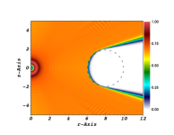
In Fig. 13, we show the radiation transport solution for the neutrino energy density. To achieve a constant value in the free streaming regime we scale the energy density by $r^{2}$. We normalize the data to range between 0 and 1. We show the solution after several light crossing times of the domain. The shadow cast by the absorbing torus is clearly seen and demonstrates this ability of our code to maintain the neutrino momentum direction. There are slight artifacts seen as ripples at larger radii and along the coordinate axes nearer to the source that arising from the first-order explicit spatial flux integration.

References

- Audit et al. (2002) Audit, E., Charrier, P., Chièze, J., & Dubroca, B. 2002, arXiv:astro-ph/0206281
- Baron & Cooperstein (1990) Baron, E., & Cooperstein, J. 1990, ApJ, 353, 597
- Bethe & Wilson (1985) Bethe, H. A., & Wilson, J. R. 1985, ApJ, 295, 14
- Bruenn (1985) Bruenn, S. W. 1985, ApJS, 58, 771
- Bruenn et al. (2001) Bruenn, S. W., De Nisco, K. R., & Mezzacappa, A. 2001, ApJ, 560, 326
- Bruenn et al. (2013) Bruenn, S. W., Mezzacappa, A., Hix, W. R., et al. 2013, ApJ, 767, L6
- Bruenn et al. (2016) Bruenn, S. W., Lentz, E. J., Hix, W. R., et al. 2016, ApJ, 818, 123
- Buras et al. (2006a) Buras, R., Janka, H.-T., Rampp, M., & Kifonidis, K. 2006a, A&A, 457, 281
- Buras et al. (2006b) Buras, R., Rampp, M., Janka, H.-T., & Kifonidis, K. 2006b, A&A, 447, 1049
- Burrows (1988) Burrows, A. 1988, ApJ, 334, 891
- Burrows et al. (2006) Burrows, A., Reddy, S., & Thompson, T. A. 2006, Nucl. Phys. A, 777, 356
- Burrows & Sawyer (1998) Burrows, A., & Sawyer, R. F. 1998, Phys. Rev. C, 58, 554
- Burrows & Sawyer (1999) —. 1999, Phys. Rev. C, 59, 510
- Burrows et al. (2016) Burrows, A., Vartanyan, D., Dolence, J. C., Skinner, M. A., & Radice, D. 2016, Accepted to Space Science Reviews, arXiv:1611.05859
- Cardall et al. (2013) Cardall, C. Y., Endeve, E., & Mezzacappa, A. 2013, Phys. Rev. D, 87, 103004
- Childs et al. (2012) Childs, H., Brugger, E., Whitlock, B., et al. 2012, in High Performance Visualization–Enabling Extreme-Scale Scientific Insight, 357–372
- Colgate & White (1966) Colgate, S. A., & White, R. H. 1966, ApJ, 143, 626
- Couch & O’Connor (2014) Couch, S. M., & O’Connor, E. P. 2014, ApJ, 785, 123
- Couch & Ott (2015) Couch, S. M., & Ott, C. D. 2015, ApJ, 799, 5
- Dolence et al. (2015) Dolence, J. C., Burrows, A., & Zhang, W. 2015, ApJ, 800, 10
- Dubey et al. (2009) Dubey, A., Reid, L. B., Weide, K., et al. 2009, Parallel Comput., 35, 512
- Ertl et al. (2016) Ertl, T., Janka, H.-T., Woosley, S. E., Sukhbold, T., & Ugliano, M. 2016, ApJ, 818, 124
- Foglizzo et al. (2006) Foglizzo, T., Scheck, L., & Janka, H.-T. 2006, ApJ, 652, 1436
- Fryxell et al. (2000) Fryxell, B., Olson, K., Ricker, P., et al. 2000, ApJS, 131, 273
- Handy et al. (2014) Handy, T., Plewa, T., & Odrzywołek, A. 2014, ApJ, 783, 125
- Hanke et al. (2012) Hanke, F., Marek, A., Müller, B., & Janka, H.-T. 2012, ApJ, 755, 138
- Horowitz (2002) Horowitz, C. J. 2002, Phys. Rev. D, 65, 043001
- Hunter (2007) Hunter, J. D. 2007, Computing In Science & Engineering, 9, 90
- Just et al. (2015) Just, O., Obergaulinger, M., & Janka, H.-T. 2015, MNRAS, 453, 3386
- Keil (1997) Keil, W. 1997, PhD thesis, Technische Universität München, Munich, Germany
- Kuroda et al. (2012) Kuroda, T., Kotake, K., & Takiwaki, T. 2012, ApJ, 755, 11
- Lattimer & Swesty (1991) Lattimer, J. M., & Swesty, F. D. 1991, Nucl. Phys. A, 535, 331
- Lentz et al. (2012) Lentz, E. J., Mezzacappa, A., Messer, O. E. B., et al. 2012, ApJ, 747, 73
- Lentz et al. (2015) Lentz, E. J., Bruenn, S. W., Hix, W. R., et al. 2015, ApJ, 807, L31
- Liebendörfer et al. (2001) Liebendörfer, M., Mezzacappa, A., Thielemann, F.-K., et al. 2001, Phys. Rev. D, 63, 103004
- Liebendörfer et al. (2005) Liebendörfer, M., Rampp, M., Janka, H.-T., & Mezzacappa, A. 2005, ApJ, 620, 840
- Loken et al. (2010) Loken, C., Gruner, D., Groer, L., et al. 2010, Journal of Physics Conference Series, 256, 012026
- Marek et al. (2006) Marek, A., Dimmelmeier, H., Janka, H.-T., Müller, E., & Buras, R. 2006, A&A, 445, 273
- Marek & Janka (2009) Marek, A., & Janka, H.-T. 2009, ApJ, 694, 664
- May & White (1966) May, M. M., & White, R. H. 1966, Phys. Rev., 141, 1232
- Melson et al. (2015) Melson, T., Janka, H.-T., Bollig, R., et al. 2015, ApJ, 808, L42
- Minerbo (1978) Minerbo, G. N. 1978, J. Quant. Spec. Radiat. Transf., 20, 541
- Misner & Sharp (1964) Misner, C. W., & Sharp, D. H. 1964, Phys. Rev., 136, 571
- Müller & Janka (2015) Müller, B., & Janka, H.-T. 2015, MNRAS, 448, 2141
- Müller et al. (2010) Müller, B., Janka, H.-T., & Dimmelmeier, H. 2010, ApJS, 189, 104
- Müller et al. (2012a) Müller, B., Janka, H.-T., & Heger, A. 2012a, ApJ, 761, 72
- Müller et al. (2012b) Müller, B., Janka, H.-T., & Marek, A. 2012b, ApJ, 756, 84
- Murphy et al. (2013) Murphy, J. W., Dolence, J. C., & Burrows, A. 2013, ApJ, 771, 52
- Nakamura et al. (2015) Nakamura, K., Takiwaki, T., Kuroda, T., & Kotake, K. 2015, PASJ, 67, 107
- O’Connor (2015) O’Connor, E. 2015, ApJS, 219, 24
- O’Connor & Couch (2015) O’Connor, E., & Couch, S. M. 2015, submitted to ApJ; arXiv:1511.07443, arXiv:1511.07443v1
- O’Connor et al. (2017) O’Connor, E., Horowitz, C., Lin, Z., & Couch, S. 2017, in Proceedings of the International Astronomical Union S331, Proceedings of the International Astronomical Union S331
- O’Connor & Ott (2010) O’Connor, E., & Ott, C. D. 2010, Class. Quantum Grav., 27, 114103
- O’Connor & Ott (2011) —. 2011, ApJ, 730, 70
- O’Connor & Ott (2013) —. 2013, ApJ, 762, 126
- Ott et al. (2008) Ott, C. D., Burrows, A., Dessart, L., & Livne, E. 2008, ApJ, 685, 1069
- Ott et al. (2013) Ott, C. D., Abdikamalov, E., Mösta, P., et al. 2013, ApJ, 768, 115
- Pan et al. (2016) Pan, K.-C., Liebendörfer, M., Hempel, M., & Thielemann, F.-K. 2016, ApJ, 817, 72
- Pan et al. (2017) Pan, K.-C., Liebendörfer, M., Hempel, M., & Thielemann, F.-K. 2017, in 14th International Symposium on Nuclei in the Cosmos (NIC2016), ed. S. Kubono, T. Kajino, S. Nishimura, T. Isobe, S. Nagataki, T. Shima, & Y. Takeda, 020703
- Radice et al. (2017) Radice, D., Burrows, A., Vartanyan, D., Skinner, M. A., & Dolence, J. C. 2017, ApJ, 850, 43
- Rampp & Janka (2002) Rampp, M., & Janka, H.-T. 2002, A&A, 396, 361
- Shen et al. (2011) Shen, H., Toki, H., Oyamatsu, K., & Sumiyoshi, K. 2011, ApJS, 197, 20
- Shibata et al. (2011) Shibata, M., Kiuchi, K., Sekiguchi, Y., & Suwa, Y. 2011, Progress of Theoretical Physics, 125, 1255
- Skinner et al. (2016) Skinner, M. A., Burrows, A., & Dolence, J. C. 2016, ApJ, 831, 81
- Summa et al. (2016) Summa, A., Hanke, F., Janka, H.-T., et al. 2016, ApJ, 825, 6
- Suwa et al. (2010) Suwa, Y., Kotake, K., Takiwaki, T., et al. 2010, Pub. Astr. Soc. Jap., 62, L49
- Suwa et al. (2016) Suwa, Y., Yamada, S., Takiwaki, T., & Kotake, K. 2016, ApJ, 816, 43
- Takiwaki et al. (2012) Takiwaki, T., Kotake, K., & Suwa, Y. 2012, ApJ, 749, 98
- Takiwaki et al. (2014) —. 2014, ApJ, 786, 83
- Thompson et al. (2003) Thompson, T. A., Burrows, A., & Pinto, P. A. 2003, ApJ, 592, 434
- Wilson (1971) Wilson, J. R. 1971, ApJ, 163, 209
- Woosley & Heger (2007) Woosley, S. E., & Heger, A. 2007, Phys. Rep., 442, 269
- Woosley et al. (2002) Woosley, S. E., Heger, A., & Weaver, T. A. 2002, \rmp, 74, 1015
- Woosley & Weaver (1995) Woosley, S. E., & Weaver, T. A. 1995, ApJS, 101, 181