The tail effect in gravitational radiation-reaction:
time non-locality and

renormalization group evolution

Chad R. Galley,¹ Adam K. Leibovich,² Rafael A. Porto³ and Andreas Ross⁴

¹ Theoretical Astrophysics (TAPIR), Walter Burke Institute for Theoretical Physics,
California Institute of Technology, Pasadena, California 91125, USA

² Pittsburgh Particle Physics Astrophysics and Cosmology Center (PITT PACC)
Department of Physics and Astronomy, University of Pittsburgh, Pittsburgh, Pennsylvania 15260, USA ³ ICTP South American Institute for Fundamental Research,
Instituto de Física Teórica - Universidade Estadual Paulista
Rua Dr. Bento Teobaldo Ferraz 271, 01140-070 São Paulo, SP Brazil ⁴ Department of Physics and Astronomy
Carnegie Mellon University, Pittsburgh, Pennsylvania 15213, USA

  Abstract
We use the effective field theory (EFT) framework to calculate the tail effect in gravitational radiation reaction, which enters at 4PN order in the dynamics of a binary system. The computation entails a subtle interplay between the near (or potential) and far (or radiation) zones. In particular, we find that the tail contribution to the effective action is non-local in time, and features both a dissipative and a ‘conservative’ term. The latter includes a logarithmic ultraviolet (UV) divergence, which we show cancels against an infrared (IR) singularity found in the (conservative) near zone. The origin of this behavior in the long-distance EFT is due to the point-particle limit –shrinking the binary to a point– which transforms a would-be infrared singularity into an ultraviolet divergence. This is a common occurrence in an EFT approach, which furthermore allows us to use renormalization group (RG) techniques to resum the resulting logarithmic contributions. We then derive the RG evolution for the binding potential and total mass/energy, and find agreement with the results obtained imposing the conservation of the (pseudo) stress-energy tensor in the radiation theory. While the calculation of the leading tail contribution to the effective action involves only one diagram, five are needed for the one-point function. This suggests logarithmic corrections may be easier to incorporate in this fashion. We conclude with a few remarks on the nature of these IR/UV singularities, the (lack of) ambiguities recently discussed in the literature, and the completeness of the analytic Post-Newtonian framework.  

1 Introduction

The effective field theory (EFT) framework introduced in [1], and coined NRGR for ‘Non-Relativistic General Relativity’, has proven to be very successful in the study of the two-body problem in general relativity. Originally, the formalism in [1] was used to derive the first Post-Newtonian correction (1PN) to the conservative dynamics for non-rotating objects. Soon after the 2PN [2] and 3PN [3] gravitational potentials were computed, reproducing previous results within traditional methods, e.g. [4, 5, 6] (see [7] for a complete list of references.) On the other hand, in the radiative sector, the 1PN [8] and 2PN [9] radiative multipoles were computed within NRGR, which is however still below the state of the art for non-spinning binary systems at 3PN order, e.g. [7]. NRGR was promptly extended in [10] to include spin degrees of freedom, and used to describe spinning compact binary systems to 3PN [10, 11, 12, 13, 14, 15, 16, 17, 18, 19, 20]. Some of these results were previously derived in [21, 22, 23, 24] for the spin-orbit sector at 2.5PN order. The spin-spin gravitational potentials to 3PN were obtained within the EFT approach in [11, 12, 13, 14, 18], and in [25, 26, 27, 28] and [29], using the Arnowitt-Deser-Misner (ADM) and harmonic gauge formalisms, respectively. The radiative multipole moments quadratic in the spin needed for the radiated power to 3PN, computed in [16] using the framework of [10, 14, 8, 30], were also obtained in [29], although the comparison is pending. The required multipoles for the gravitational wave amplitude to 2.5PN order were computed in [17], see also [31]. Higher order effects have been incorporated in the conservative sector. In [32, 33, 34, 35] the gravitational spin-orbit and spin-spin potentials were computed at 3.5PN and 4PN order, respectively. These results were derived with more traditional methods in [36, 37, 38], except for finite-size effects [34], which are more efficiently handled in an EFT framework [1, 10, 14]. The formalism in [10, 14] was also used to compute the leading finite size effects cubic (and quartic) in the spin in [39, 40, 41]. In conjunction, all of these results augment the knowledge of the dynamics of binary compact objects to 4PN order. For thorough reviews on the two-body problem and the EFT approach see [7, 42, 43, 44, 45, 46, 47].

The computation of the (local part of the) spin independent 4PN potential, at next-to-next-to-next-to-next-to leading order beyond the Newtonian approximation, was recently culminated in [48, 49, 50, 51] and [52] using the ADM and harmonic formalisms, respectively. A partial result computed in NRGR [53] has shown full agreement. However, the subtleties associated with infrared (IR) and ultraviolet (UV) divergences, which appear at this order, have led to a disagreement between different approaches [52, 54]. As we shall see, the present paper partially addresses some of these issues –in particular the (lack of) ambiguities and completeness of the PN framework– pending the completion of the full 4PN conservative dynamics within NRGR. At 4PN order there is also a contribution to the effective action which is non-local in time, e.g. [7, 55], recently revisited in [51, 52], as well as logarithmic corrections to the binding mass/energy. The latter were obtained within NRGR in [56] through the conservation of the (pseudo) stress-energy tensor in the radiation zone, and in full agreement with a previous computation in [57]. Both of these results feature prominently in this work, but instead arise from the computation of radiation-reaction effects.

The study of time-irreversible back-reaction effects within the EFT formalism was initiated in [58] in the extreme mass ratio limit, and in[59] for NRGR, by implementing the classical limit of the ‘in-in’ formalism, e.g. [60, 61]. Later, the radiation-reaction force to 3.5PN order [62, 63] was rederived within the EFT approach in [64] using a framework that extends Hamilton’s principle to generic nonconservative systems [65, 66]. These results are obtained at leading order in $G_{N}$ in the radiation theory. In the present work we incorporate non-linear effects in the radiation zone by computing the tail contribution, e.g. [67, 68, 69, 70, 71], to the effective action. We will find that the tail contribution plays an essential role in both the results mentioned above, namely, the presence of logarithms and time non-locality.

The non-linear couplings due to the higher order tails in gravitational wave emission produce divergences. The IR singularities (which are also present in the leading tail contribution) exponentiate into an overall phase in the amplitude [8], which drops out of the total radiated power or can be removed from the gravitational waveform via a time redefinition [17]. On the other hand, the UV divergences thus far have been properly renormalized through counter-terms in the radiation theory, which led to renormalization group (RG) trajectories for the binding mass/energy and multipole moments, described in [8, 56]. As we discuss here, similar behavior unfolds through the study of radiation-reaction effects, albeit involving a subtle interplay between the theory of potential modes (near zone) and the radiation sector (far zone).

The radiation-reaction force corrects the dynamics of the constituents of the binary system at the orbit scale, $r$. However, we compute it by integrating out the radiation field, $\bar{h}_{\mu\nu}$, with a long-distance effective action [8, 30]

$$S_{\rm eff}^{\rm rad}[{\bm{x}}_{a},\bar{h}_{\mu\nu}]=-\int dt\sqrt{\bar{g}_{00}} \bigg{[}M(t)-\sum_{\ell=2}\bigg{(}\frac{1}{\ell!}I^{L}(t)\nabla_{L-2}E_{i_{\ell-1}i_{\ell}}$$

$$+\frac{2\ell}{(2\ell+1)!}J^{L}(t)\nabla_{L-2}B_{i_{\ell-1}i_{\ell}}\bigg{)}\bigg{]}\,,$$

where radiation modes vary on scales of order $\lambda_{\rm rad}\sim r/v\gg r$ and propagate on a background (Schwarzschild) geometry sourced by the first term, $M$, which at leading order gives a potential,

$$\Phi({\bm{q}})\simeq-\frac{G_{N}M}{{\bm{q}}^{2}}\,.$$ (1.2)

Therefore, the study of radiation reaction entails the interaction between different zones. This is even more relevant when the tail contribution is incorporated, as we show here.

After integrating out the radiation field, including the tail effect, we will find that the resulting effective action for the dynamics of the binary is non-local in time, in agreement with a recent claim in [51]. We also find both dissipative and ‘conservative’ contributions, and the latter includes the presence of a logarithmic UV divergence. Hence, unlike the renormalization of the one-point function in [8, 56] which occurs in the radiation zone, the counter-term for this divergence must originate in the potential region. We argue this involves the existence of an IR singularity in the near zone. This is expected because the radiation-reaction potential is now part of the dynamics at short(er) distances. Moreover, UV divergences in the theory of potentials are removed by counter-terms in the worldline theory for each constituent in the binary and, because of the ‘effacement theorem,’ do not contribute until 5PN order (for non-rotating bodies). The seed of the UV divergence in the tail computation is the point-particle limit, implicitly taken in (1), where the binary as a whole is treated as a point-like source. By shrinking the binary to a point we transform a would-be IR singularity into a UV divergence. This is a common occurrence in an EFT approach that, furthermore, allows us to use RG techniques to resum the resulting logarithmic contributions. We then derive the RG evolution for the binding potential and total mass/energy and find agreement with the results obtained in [56]. While the calculation of the radiation-reaction potential involves computing only one diagram, five are needed for the one-point function in [56], which suggests higher order logarithmic terms may be easier to incorporate in this fashion.

This paper is organized as follows. We first review the computation of radiation-reaction effects within NRGR. We then integrate out the radiation field including the tail effect, and demonstrate the presence of dissipative and conservative terms, and the time non-locality of the effective action. Afterwards we discuss renormalization and RG equations. We conclude with a few remarks on the breakdown of the separation of scales, the origin of the ambiguities recently discussed in the literature, e.g. [54], and the completeness of the analytic PN framework. The computation of the tail effect in the radiation-reaction potential within the EFT formalism was first approached in [72]. We also comment at the end on the main differences between [72] and the present work. We relegate details of the computation to an appendix.

2 Gravitational radiation-reaction in NRGR

Accommodating the time-asymmetric interactions associated with nonconservative processes, like radiation reaction, at the level of the action entails formally doubling the degrees of freedom in the problem so that ${\bm{x}}_{a}\to\{{\bm{x}}^{(1)}_{a},{\bm{x}}^{(2)}_{a}\}$, with ${\bm{x}}_{a}$ being the physical coordinates of the $a^{\rm th}$ body, and similarly for the radiative metric perturbations, $\bar{h}_{\mu\nu}\to\{\bar{h}_{\mu\nu}^{(1)},\bar{h}_{\mu\nu}^{(2)}\}$. After the latter are integrated out from the theory, we will be left with an effective action that can be written as

$$W[{\bm{x}}^{\pm}_{a}]=\int dt\,\big{(}L[{\bm{x}}_{a}^{(1)}]-L[{\bm{x}}_{a}^{(2)}]+R[{\bm{x}}_{a}^{(1)},{\bm{x}}_{a}^{(2)}]\big{)},$$ (2.1)

where $L=\int dt(K-V)$ is the usual Lagrangian that accounts for the binary’s conservative interactions while $R$ accommodates non-conservative effects, such as radiation reaction. It is worth noticing that if $R$ contains terms that can be written in a manner resembling the first two terms, namely,

$$R[{\bm{x}}_{a}^{(1)},{\bm{x}}_{a}^{(2)}]\supset F[{\bm{x}}_{a}^{(1)}]-F[{\bm{x}}_{a}^{(2)}],$$ (2.2)

then $F$ may be absorbed into a redefinition of $L$ and, ultimately, the conservative binding potential [65]. This observation will be important later on when we discuss the tail effect in Sec. 3. Details of the underlying theory of general nonconservative mechanics is given in [65] and extended to field theories and continuum systems (including viscous fluid flows with entropy production) in [66].

The leading contribution to the radiation reaction force comes from the following diagram in the effective action [59],

$$\begin{aligned} iW[{\bm{x}}^{\pm}_{a}]&=\parbox{59.75078pt}{\includegraphics[width=91.9986pt]{LOSF.pdf}}\\ &=\left(\frac{1}{2}\right)\left(\frac{i}{2{M_{\rm Pl}}}\right)^{2}\int dt\int dt^{\prime}I_{A}^{ij}(t)\big{\langle}E^{A}_{ij}(t,{\bm{0}})E^{B}_{kl}(t^{\prime},{\bm{0}})\big{\rangle}I_{B}^{kl}(t^{\prime}),\end{aligned}$$ (2.3)

where $A,B=\pm$, ${\bm{x}}_{a+}\equiv({\bm{x}}_{a}^{(1)}+{\bm{x}}_{a}^{(2)})/2$, and ${\bm{x}}_{a-}\equiv{\bm{x}}_{a}^{(1)}-{\bm{x}}_{a}^{(2)}$. The tensor $E_{ij}(t,{\bm{0}})$ is the electric part of the Weyl curvature tensor evaluated at the binary’s center of mass, which is taken to be at the origin. The equations of motion are found from the effective action through

$$\left[\frac{\delta W}{\delta{\bm{x}}^{i}_{a-}(t)}\right]_{\rm PL}=0\qquad\Longrightarrow\qquad\frac{d}{dt}\frac{{\partial}L}{{\partial}{\bm{x}}^{i}_{a}}-\frac{{\partial}L}{{\partial}{\bm{x}}^{i}_{a}}=\bigg{[}\frac{{\partial}R}{{\partial}{\bm{x}}^{i}_{a-}}-\frac{d}{dt}\frac{{\partial}R}{{\partial}{\bm{v}}^{i}_{a-}}\bigg{]}_{\rm PL}\,,$$ (2.4)

where “PL” indicates the physical limit wherein ${\bm{x}}_{a-}\to 0$ and ${\bm{x}}_{a+}\to{\bm{x}}_{a}$. The two-point function in the harmonic gauge for trace-reversed metric perturbations is given by

$$\big{\langle}E^{A}_{ij}(t,{\bm{0}})E^{B}_{kl}(t^{\prime},{\bm{0}})\big{\rangle}=-\frac{i}{8}\bigg{[} {\partial}_{i}{\partial}_{j}{\partial}_{k^{\prime}}{\partial}_{l^{\prime}}+2P_{ijkl}{\partial}_{0}^{2}{\partial}_{0^{\prime}}^{2}-\eta_{ij}{\partial}_{0}^{2}{\partial}_{k^{\prime}}{\partial}_{l^{\prime}}-\eta_{kl}{\partial}_{i}{\partial}_{j}{\partial}_{0^{\prime}}^{2}+\eta_{ik}{\partial}_{j}{\partial}_{0}{\partial}_{l^{\prime}}{\partial}_{0^{\prime}}{}$$

$$+\eta_{jl}{\partial}_{i}{\partial}_{0}{\partial}_{k^{\prime}}{\partial}_{0^{\prime}}+\eta_{il}{\partial}_{j}{\partial}_{0}{\partial}_{k^{\prime}}{\partial}_{0^{\prime}}+\eta_{jk}{\partial}_{i}{\partial}_{0}{\partial}_{l^{\prime}}{\partial}_{0^{\prime}}\bigg{]}G^{AB}(t-t^{\prime},{\bm{0}}),$$ (2.5)

where the prime on a spacetime index of a derivative is taken with respect to $x^{\prime}{}^{\mu}$, and

$$P_{\alpha\beta\gamma\delta}=\frac{1}{2}\big{(}\eta_{\alpha\gamma}\eta_{\beta\delta}+\eta_{\alpha\delta}\eta_{\beta\gamma}-\eta_{\alpha\beta}\eta_{\gamma\delta}\big{)}.$$ (2.6)

The matrix of propagators in the $\pm$ variables is

$$G^{AB}(x^{\mu}-x^{\prime}{}^{\mu})=\left(\begin{array}[]{cc}0&G_{\rm adv}(x^{\mu}-x^{\prime}{}^{\mu})\\ G_{\rm ret}(x^{\mu}-x^{\prime}{}^{\mu})&0\end{array}\right),$$ (2.9)

with $G^{-+}(x^{\mu}-x^{\prime}{}^{\mu})=G_{\rm ret}(x^{\mu}-x^{\prime}{}^{\mu})$. The two propagators are needed to enforce the causal (i.e., outgoing) boundary conditions on the metric perturbations being integrated out [65].

Computing the diagram in (2.3) results in [59]

$$W[{\bm{x}}_{a}^{\pm}]=-\frac{G_{N}}{5}\int dt\,I_{-}^{ij}(t)I_{+ij}^{(5)}(t)\equiv\int dt\,R_{\rm rad}[{\bm{x}}_{a}^{\pm}],$$ (2.10)

where the superscript $(5)$ indicates five time derivatives and we introduced

$$I_{-}^{ij}(t) \equiv I^{ij}(t;{\bm{x}}_{a}^{(1)})-I^{ij}(t;{\bm{x}}_{a}^{(2)})=\sum_{a}m_{a}\left({\bm{x}}_{a-}^{i}{\bm{x}}_{a+}^{j}+{\bm{x}}_{a+}^{i}{\bm{x}}_{a-}^{j}-\frac{2}{3}\,\delta^{ij}{\bm{x}}_{a-}\!\cdot\!{\bm{x}}_{a+}\right)+{\cal O}({\bm{x}}_{a-}^{3}),{}$$

$$I_{+}^{ij}(t) \equiv\frac{1}{2}\Big{(}I^{ij}(t;{\bm{x}}_{a}^{(1)})+I^{ij}(t;{\bm{x}}_{a}^{(2)})\Big{)}=\sum_{a}m_{a}\left({\bm{x}}_{a+}^{i}{\bm{x}}_{a+}^{j}-\frac{1}{3}\delta^{ij}{\bm{x}}_{a+}^{2}\right)+{\cal O}({\bm{x}}_{a-}^{2}).$$ (2.11)

Using (2.4) we obtain the acceleration on the $a^{\rm th}$ body resulting from (2.10) as [59]

$$({\bm{a}}^{i}_{a})_{\rm rr}(t)=-\frac{2G_{N}}{5}I^{(5)ij}(t){\bm{x}}_{a}^{j}(t).$$ (2.12)

This is precisely the radiation-reaction force derived by Burke and Thorne [73, 74]. At this order, notice that $R_{\rm rad}$ defined in (2.10) cannot be absorbed into a redefinition of the binding potential and thus represents a truly non-conservative effect. The action for the conservative sector of the theory (i.e., ‘turning off’ radiative effects) is invariant under time translations implying the existence of a conserved quantity, namely, the binary’s binding mass/energy,

$$M\equiv\sum_{a}{\bm{v}}_{a}\cdot\frac{{\partial}L}{{\partial}{\bm{v}}_{a}}-L\,.$$ (2.13)

Once radiation is turned on, $M$ is no longer conserved since $R[{\bm{x}}_{a}^{\pm}]$ accounts for time-irreversible interactions[66, 47]. Hence, we have

$$\dot{M}=\sum_{a}{\bm{v}}_{a}\cdot\bigg{[}\frac{{\partial}R}{{\partial}{\bm{x}}_{a-}}-\frac{d}{dt}\frac{{\partial}R}{{\partial}{\bm{v}}_{a-}}\bigg{]}_{\rm PL}.$$ (2.14)

For the case of gravitational radiation reaction, using $R_{\rm rad}$ from (2.10) we find

$$\dot{M}=-\frac{G_{N}}{5}I^{(1)ij}(t)I^{(5)ij}(t)\,,$$ (2.15)

at leading PN order. Notice, after some simple algebraic manipulations, we can write (2.15) as

$$\dot{E}=-\frac{G_{N}}{5}{I}^{(3)ij}(t)I^{(3)ij}(t)\,,$$ (2.16)

where

$$E=M+\frac{G_{N}}{5}I^{(1)ij}(t)I^{(4)ij}(t)-\frac{G_{N}}{5}{I}^{(2)ij}(t)I^{(3)ij}(t)\,.$$ (2.17)

The extra pieces are analogous to the Schott energy in electrodynamics, and may be interpreted in terms of near-zone contributions from the metric perturbations [47].

We then average (2.15) over a bound (not necessarily circular) orbit and find that the Schott-like terms average away leaving behind the well-known quadrupole formula,

$$\big{\langle}\dot{M}\big{\rangle}=-P_{LO}=-\frac{G_{N}}{5}\big{\langle}{I}^{(3)ij}(t)I^{(3)ij}(t)\big{\rangle}\,.$$ (2.18)

The above result was also derived through the conservation of the (pseudo) stress-energy tensor in [56].

The previous steps can be generalized to all $\ell$-order radiative multipoles. The diagrams contributing to the effective action are

$$iW[{\bm{x}}_{a}^{(\pm)}]\,=\,\sum_{\ell\geq 2}\leavevmode\nobreak\ \leavevmode\nobreak\ \parbox{59.75078pt}{\includegraphics[width=206.9986pt]{LOSFL.pdf}}{}$$

and are found to give

$$\begin{aligned} W[{\bm{x}}_{a}^{\pm}]=G_{N}\sum_{\ell\geq 2}\frac{(-1)^{\ell+1}(\ell+2)}{(\ell-1)}\int dt\,\bigg{(}&\frac{2^{\ell}(\ell+1)}{\ell(2\ell+1)!}I_{-}^{L}(t)I_{+}^{L\,(2\ell+1)}(t)\\ &+\frac{2^{\ell+3}\ell}{(2\ell+2)!}J_{-}^{L}(t)J_{+}^{L\,(2\ell+1)}(t)\bigg{)}\,,\end{aligned}$$ (2.19)

which incorporates back-reaction effects at leading order in $G_{N}$ in the far zone. From (2.19) one can derive any quantity of interest in the radiation region at linear order in $G_{N}$, such as the corresponding radiation-reaction forces and orbit-averaged balance equations for energy and angular momentum for compact binary inspirals.

3 The tail effect

We now move on to incorporating non-linear gravitational interactions in the radiation zone, and the contribution from the tail effect to the radiation-reaction potential. The relevant Feynman diagram is shown in Fig. 1. We first demonstrate the time non-locality, together with the existence of dissipative and conservative contributions, to the effective action. Subsequently we discuss the renormalization and RG evolution equations.

3.1 Time non-locality

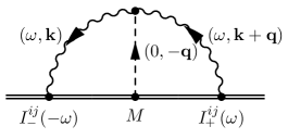
Figure 1: Feynman diagram for the tail contribution to the radiaction-reaction force. The $M$ in the tail correction may be taken as the leading averaged binding mass/energy, since the scale (and time) dependence enters at higher orders.

The resulting two-loop integral(s) arising from Fig. 1 can be written schematically as

$$iW_{\rm tail}=\int\frac{d\omega}{2\pi}\int_{{\bm{k}},{\bm{q}}}MI^{ij}_{-}(-\omega)I^{ij}_{+}(\omega)V_{\bar{h}\bar{h}\Phi}(\omega,{\bm{k}},{\bm{q}})\frac{i}{-{\bm{q}}^{2}}\frac{i}{(\omega+i\epsilon)^{2}-{\bm{k}}^{2}}\frac{i}{(\omega+i\epsilon)^{2}-({\bm{k}}+{\bm{q}})^{2}}\,.$$ (3.1)

Here, $V_{\bar{h}\bar{h}\Phi}$ represents the three-graviton coupling, and $\int_{\bm{p}}\equiv\int\frac{d^{3}{\bm{p}}}{(2\pi)^{3}}$. Notice the retarded boundary conditions in the pole structure of the propagators. We use dimensional regularization (dim. reg.) and, after some laborious manipulations outlined in App. A, we arrive at

$$iW_{\rm tail}[{\bm{x}}_{a}^{\pm}]=-i\int\frac{d\omega}{2\pi}\,\frac{(d-3)M\omega^{4}\,I_{-}^{ij}(-\omega)I_{+}^{ij}(\omega)}{32(d-2)^{2}(d-1)(d+1)}\Big{[}(d^{2}-2d+3)I_{0}-\frac{d(d-2)(d-1)}{d-4}\omega^{2}J_{0}\Big{]}\,,$$ (3.2)

in terms of two $d$-dimensional integrals, $I_{0}$ and $J_{0}$, see (A.16)-(A.17). The result is UV divergent. Expanding around $d=4$ we find,

$$W_{\rm tail}[{\bm{x}}_{a}^{\pm}]=\,\frac{2G_{N}^{2}M}{5}\int_{-\infty}^{\infty}\frac{d\omega}{2\pi}\,\omega^{6}\,I_{-}^{ij}(-\omega)I_{+}^{ij}(\omega)\bigg{[} -\frac{1}{(d-4)_{\rm UV}}-\gamma_{E}+\log\pi{}$$

$$-\log\frac{\omega^{2}}{\mu^{2}}+\frac{41}{30}+i\pi\,\text{sign}(\omega)\bigg{]}.$$ (3.3)

The pole is removed by a counter-term (see below) and we obtain

$$W_{\rm tail}[{\bm{x}}_{a}^{\pm}] =-\frac{2G_{N}^{2}M}{5}\int\frac{d\omega}{2\pi}\,\omega^{6}\,I_{-}^{ij}(-\omega)I_{+}^{ij}(\omega)\left[\log\frac{\omega^{2}}{\mu^{2}}-i\pi\,\text{sign}(\omega)\right]\,,$$ (3.4)

where we also absorbed a constant piece into a redefinition of $\mu$. We can now Fourier transform from frequency space back to the time domain, yielding

$$W_{\rm tail}[{\bm{x}}_{a}^{\pm}]=\frac{4G_{N}^{2}M}{5}\Big{(} {\rm PV}\int dt\,I_{-}^{(3)ij}(t)\int_{-\infty}^{t}dt^{\prime}\,I_{+}^{ij(3)}(t^{\prime})\left[\frac{1}{t-t^{\prime}}\right]$$ (3.5)

$$+\,\int dt\,I_{-}^{(3)ij}(t)I_{+}^{ij(3)}(t)\log\mu\Big{)}\equiv\int dt\,R_{\rm tail}[{\bm{x}}_{a}^{\pm}]{}\,,$$

where ‘PV’ stands for Principal Value. We can also write the effective action as,

$$W_{\rm tail}[{\bm{x}}^{\pm}_{a}]=\frac{4G_{N}^{2}M}{5}\leavevmode\nobreak\ {\rm PV}\int dt\,I_{-}^{(3)ij}(t)\int_{-\infty}^{t}dt^{\prime}\,I_{+}^{ij(4)}(t^{\prime})\log(|{t-t^{\prime}}|\mu)\,.$$ (3.6)

This result is formally equivalent to the non-local term discussed in [51, 54] and [52] (see also [55]).

3.2 Conservative and dissipative terms

It is easy to see that all the terms in (3.3) are of the form in (2.2) except for the one involving $\text{sign}(\omega)$. (This is clear since it is the only term that is not invariant under $\omega\to-\omega$.) Therefore, $W_{\rm tail}$ contains both conservative and dissipative interactions. In particular, the pole and logarithm terms are both part of the conservative sector and consequently renormalize the binary’s binding mass/energy. This implies that the RG structure of the theory, which we discuss in the next sub-section, occurs entirely in the conservative sector and the dissipative term is finite.

From the expressions in (3.5) (or (3.6)) and (2.4), we then derive the contribution due to the conservative and non-conservative terms to the radiation-reaction acceleration,

$$\left({\bm{a}}^{j}_{a}\right)_{\rm rr,tail}(t)=\left({\bm{a}}^{j}_{a}\right)_{{\rm cons}}(t,\mu)+\left({\bm{a}}^{j}_{a}\right)_{{\rm diss}}(t)\,,$$ (3.7)

where

$$\left({\bm{a}}^{j}_{a}\right)_{{\rm cons}}(t,\mu) = -\frac{4G_{N}^{2}M}{5}\,{\bm{x}}_{a}^{i}(t)\left(I^{ij(6)}(t)\log\mu^{2}+{\rm PV}\int_{-\infty}^{\infty}dt^{\prime}\,I^{ij(6)}(t^{\prime})\left[\frac{1}{|t-t^{\prime}|}\right]\right)\,,$$ (3.8)

$$\left({\bm{a}}^{j}_{a}\right)_{{\rm diss}}(t) = -\frac{4G_{N}^{2}M}{5}\,{\bm{x}}_{a}^{i}(t)\leavevmode\nobreak\ {\rm PV}\int_{-\infty}^{\infty}dt^{\prime}\,I^{ij(6)}(t^{\prime})\left[\frac{1}{t-t^{\prime}}\right]\,.$$ (3.9)

Notice both combine to a causality-preserving force, as expected. In other words, the presence of both conservative and non-conservative terms guarantees the integral in (3.5) (and (3.6)) only receives contributions from $t^{\prime}<t$.

3.3 Renormalization

3.3.1 Counter-term

After using dim. reg., the computation of the tail effect in gravitational radiation reaction contains a UV pole. Therefore, we require a counter-term to remove the divergence when $d\to 4$. Since the pole appears in the conservative sector (see above) we require the following counter-term

$$-\int dt\,V_{\rm ct}[{\bm{x}}_{a}]=\,\,\frac{1}{(d-4)_{\rm UV}}\frac{G_{N}^{2}M}{5}\int dt\,I^{(3)ij}(t)I^{(3)ij}(t)\,.$$ (3.10)

(Note the expression in (3.10) is half of the one in (3.3). This occurs after translating from the minus to the standard variables.)

The origin of this counter-term, however, is subtle. That is because the divergence in (3.10) cannot be associated with short-distance behavior in the theory of potentials, which are instead responsible for finite size effects for extended objects. Moreover, the leading order finite size effects for (non-rotating) binary systems enters at 5PN, e.g. [47, 46], whereas (3.10) contributes at 4PN order. Nevertheless, the UV divergence in (3.3) arises in a point-particle limit, the one in which we shrunk the binary to a point-like source, by sending the separation between constituents to zero (represented by the double line in Fig. 1). However, the separation is kept finite at the orbital scale since it is the typical scale of variation of the potential modes. For the latter, modes in the radiation zone are soft(er). Therefore, it is natural to expect the UV divergence in (3.3) to be related to an IR singularity at the orbital scale. Indeed, the existence of such an IR divergence in the theory of potentials was recently found in [50, 51, 52], in both the ADM and harmonic frameworks. The resulting potential, $V_{\rm 4pn}$, may be then split into a local term and IR-dependent pieces [50, 51]

$$V_{\rm 4pn}[{\bm{x}}_{a}] = V_{\rm 4pn}[{\bm{x}}_{a},\tilde{\mu}]-\frac{1}{(d-4)_{\rm IR}}\frac{G_{N}^{2}M}{5}I^{(3)ij}(t)I^{(3)ij}(t)\,,$$ (3.11)

using dim. reg., with

$$V_{\rm 4pn}[{\bm{x}}_{a},\tilde{\mu}] = V_{\rm 4pn}^{\rm local}[{\bm{x}}_{a}]+\frac{2G_{N}^{2}M}{5}I^{(3)ij}(t)I^{(3)ij}(t)\log\tilde{\mu}r\,,$$ (3.12)

where $r\equiv|{\bm{x}}_{1}-{\bm{x}}_{2}|$, and up to a rescaling of $\tilde{\mu}$ to absorb some extra constants.  While the form of $V_{\rm 4pn}^{\rm local}[{\bm{x}}_{a}]$ depends on the choice of gauge, the coefficient of the logarithm is physical (and gauge invariant to this order) since, as we shall see, it contributes to the total binding/mass energy of the binary system. Therefore, as we see in (3.11), the computations in [50, 51, 49, 52] provide the counter-term needed to cancel the divergence in $W_{\rm tail}$. We have distinguished $\tilde{\mu}$ from $\mu$ to emphasize the arbitrariness of the renormalization procedure and the choice of subtraction scale, both at the orbital and radiation zones. We return to this issue in sec. 4.

3.3.2 Renormalization group flow

After the divergences are subtracted away, the effective action becomes a function of a renormalized Lagrangian, and is given (in frequency space) by

$$W[{\bm{x}}_{a}^{\pm}]=\int\frac{d\omega}{2\pi}\Bigg{(} L_{\rm ren}[{\bm{x}}_{a}^{(1)};\omega,\mu]-L_{\rm ren}[{\bm{x}}_{a}^{(2)};\omega,\mu]{}$$

$$-\frac{2G_{N}^{2}M}{5}\omega^{6}\,I_{-}^{ij}(-\omega)I_{+}^{ij}(\omega)\left[\log\frac{\omega^{2}}{\mu^{2}}-i\pi\text{sign}(\omega)\right]\Bigg{)},$$ (3.13)

where

$$L_{\rm ren}[{\bm{x}}_{a};\omega,\mu]\equiv K[{\bm{x}}_{a};\omega]-V_{\rm ren}[{\bm{x}}_{a};\omega,\mu]\,,$$ (3.14)

after including the binary’s kinetic term, $K$. We can then read off the RG evolution equation from the $\mu$-independence of the effective action,

$$\mu\frac{\partial}{\partial\mu}W[{\bm{x}}_{a}^{\pm}]=0\leavevmode\nobreak\ \leavevmode\nobreak\ \Longrightarrow\leavevmode\nobreak\ \leavevmode\nobreak\ \mu\frac{\partial}{\partial\mu}V_{\rm ren}[{\bm{x}}^{\pm}_{a};\omega,\mu]=\frac{4G_{N}^{2}M}{5}\omega^{6}I_{-}^{ij}(-\omega)I_{+}^{ij}(\omega)\,,$$ (3.15)

In terms of the standard variables and Fourier transforming back to the time domain, we find the equivalent expression

$$\mu\frac{\partial}{\partial\mu}V_{\rm ren}[{\bm{x}}_{a};t,\mu]=\frac{2G_{N}^{2}M}{5}I^{(3)ij}(t)I^{(3)ij}(t)\,.$$ (3.16)

We may consider, for instance, the case of circular orbits. Then, choosing $\mu\simeq\lambda_{\rm rad}^{-1}$ together with $\mu_{0}\simeq r^{-1}$ for the matching scale, we find (using $\mu/\mu_{0}\simeq v$)

$$V_{\rm ren}[{\bm{x}}_{a};t,\mu]=V_{\rm ren}[{\bm{x}}_{a};t,\mu_{0}]+\frac{2G_{N}^{2}M}{5}I^{(3)}_{ij}(t)I^{(3)}_{ij}(t)\log v\,.$$ (3.17)

This expression is in accordance with the results in [51]. The renormalized potential at $\mu_{0}\simeq 1/r$ must be obtained by matching at the orbital scale. We may proceed as follows. First, notice that by choosing $\tilde{\mu}\simeq 1/r$ in (3.12) we remove the logarithmic contribution. Then, after matching, we get

$$V_{\rm ren}[{\bm{x}}_{a};t,\mu_{0}\sim 1/r]=V_{\rm 4pn}^{\rm local}[{\bm{x}}_{a}]+C\,\frac{2G_{N}^{2}M}{5}\,I^{(3)ij}(t)I^{(3)ij}(t)\,.$$ (3.18)

The factor of $C\equiv\log(\tilde{\mu}/\mu_{0})\sim 1$ accounts for the arbitrariness in the choice of renormalization schemes. The value of $C$ may be obtained, for instance, by comparison with a numerical computation or (semi-) analytically through the self-force program, e.g. [51, 76]. For example, according to [51] one finds $C_{\rm ADM}=-\tfrac{1681}{1536}$ in the ADM formalism. A similar constant, $\alpha=\tfrac{811}{672}$, appears in the harmonic framework [52]. The existence of this arbitrariness signals the breakdown of the separation of scales between potential and radiation regions. However, this breakdown does not necessarily mean additional information is needed, as advocated in [54]. On the contrary, it is instead a signature of ‘double-counting.’ Once this is properly addressed, no extra matching condition is necessary. We add a few extra remarks in sec. 4, and will elaborate further on this point elsewhere [77].Despite this fact, we can still use the EFT computation to extract information about the dynamics, including logarithmic contributions to the binding mass/energy, which are universal. Concentrating on the conservative piece, and using (2.14) together with (3.8), we may write an energy balance equation

$$\dot{M}_{\rm ren}(t,\mu)=\sum_{a}m_{a}\left({\bm{a}}_{a}\right)_{{\rm cons}}\cdot{\bm{v}}_{a}+\cdots=\frac{2G_{N}^{2}M}{5}\,I^{ij(1)}(t)\int\frac{d\omega}{2\pi}I^{ij(6)}(\omega)e^{i\omega t}\log\frac{\omega^{2}}{\mu^{2}}+\cdots\,,$$ (3.19)

where the renormalized binding mass/energy is given by, see (2.13),

$$M_{\rm ren}(t,\mu)\equiv\sum_{a}{\bm{v}}_{a}\cdot\frac{{\partial}}{{\partial}{\bm{v}}_{a}}L_{\rm ren}[{\bm{x}}_{a};t,\mu]-L_{\rm ren}[{\bm{x}}_{a};t,\mu]\,.$$ (3.20)

The ellipsis in (3.19) include also other (non-conservative) terms responsible for the power loss on gravitational wave emission, as we discussed in the previous section. We then return to the case of circular orbits with angular frequency $\Omega$ and take a time average. As it was discussed in [8], the multipole moments have support at the typical scale of gravitational wave radiation, $\lambda_{\rm rad}^{-1}\simeq 2\Omega$, so that $I^{ij}(\omega)\propto\delta(\omega\pm 2\Omega)$. Hence, (3.19) becomes

$$\left\langle\dot{M}_{\rm ren}(t,\mu)\right\rangle=-\frac{4G_{N}^{2}M}{5}\,\left\langle I^{ij(1)}(t)I^{ij(6)}(t)\right\rangle\,\log\,(\lambda_{\rm rad}\mu)+\cdots\,.$$ (3.21)

From here, using

$$I^{(1)}_{ij}(t)I^{(6)}_{ij}(t)=\frac{d}{dt}\left(I^{(5)}_{ij}(t)I^{(1)}_{ij}(t)-I^{(4)}_{ij}(t)I^{(2)}_{ij}(t)+\tfrac{1}{2}I^{(3)}_{ij}(t)I^{(3)}_{ij}(t)\right)\,,$$ (3.22)

on the right-hand side of (3.19), we get for the conservative binding energy,

$$E\equiv M_{\rm ren}(t,\mu)+\frac{2G_{N}^{2}M}{5}\left(2I^{(5)}_{ij}(t)I^{(1)}_{ij}(t)-2I^{(4)}_{ij}(t)I^{(2)}_{ij}(t)+I^{(3)}_{ij}(t)I^{(3)}_{ij}(t)\right)\,\log\,(\lambda_{\rm rad}\mu)\,.$$ (3.23)

Notice, at the radiation scale we have $E=M_{\rm ren}(t,\mu\simeq\lambda_{\rm rad}^{-1})$, as expected. From (3.23) we can read off the RG flow, after time averaging, to find

$$\mu\frac{d}{d\mu}\langle E\rangle=0\qquad\Longrightarrow\qquad\mu\frac{d}{d\mu}\left\langle M_{\rm ren}(t,\mu)\right\rangle=-2G_{N}^{2}M\left\langle I^{(3)}_{ij}(t)I^{(3)}_{ij}(t)\right\rangle\,.$$ (3.24)

This expression is in agreement with the result in [56], and leads to

$$\langle E\rangle=\left\langle M_{\rm ren}(t,\mu_{0}\simeq r^{-1})\right\rangle-2G_{N}^{2}M\left\langle I^{(3)}_{ij}(t)I^{(3)}_{ij}(t)\right\rangle\log v\,.$$ (3.25)

The 4PN logarithmic correction in the last term was first discussed in [57].

Gathering all the pieces, we finally arrive at a balanace equation of the sort,

$$\langle\dot{E}(t)\rangle=-P_{\rm local}-\frac{2G_{N}^{2}M}{5}\,\left\langle I^{ij(1)}(t)\leavevmode\nobreak\ {\rm PV}\,\int_{-\infty}^{\infty}dt^{\prime}\,I^{ij(6)}(t^{\prime})\left[\frac{1}{t-t^{\prime}}\right]\right\rangle\,,$$ (3.26)

including the non-conservative part of the tail from (3.9). Here, $P_{\rm local}$ represents the power loss induced by all other (local) dissipative terms (e.g., from Sec. 2). Performing the time average using the leading expression for the quadrupole moment on a circular orbit with frequency $\Omega$, we recover the leading contribution to the power loss due to the tail effect, e.g. [8],

$$\frac{P_{\rm tail}}{P_{LO}}=4\pi x^{3/2}\,.$$ (3.27)

Here $x\equiv(G_{N}M\Omega)^{2/3}$ is the standard PN expansion parameter. Notice the relevant factors of $\pi$, which now appear through the study of radiation-reaction effects, but without the associated IR divergences discussed in [8]. See next for more on this issue.

4 Discussion

In this paper we computed the tail contribution to the gravitational radiation reaction to 4PN order within the EFT framework. We arrived at an effective action that displays time non-locality, i.e. (3.5), contribuiting conservative as well as dissipative terms to the radiation-reaction force, i.e. (3.8) and (3.9), respectively. The former being responsible for non-trivial RG trajectories for the gravitational binding potential and mass/energy in the near zone, i.e. (3.16) and (3.24), while the latter leads to the well-known power loss due to the leading tail effect, i.e. (3.27).

Given the nature of the computation, naively, one would have thought that the tail contribution to the effective action could have been obtained by replacing the source quadrupole moment in the Burke-Thorne result (2.12), with the corresponding radiative moment induced by the tail effect, e.g. [8, 16]. However, while the leading tail contribution to the radiative quadrupole presents an IR divergence [8, 16], we find here instead a UV singularity, i.e. (3.3). As we argued, the singular behavior in the tail contribution to the effective action stems off the conservative sector. The UV pole is thus ultimately canceled by a counter-term in the near zone, but arising from an IR divergence [50, 51, 49]. This is consistent with the expectation that the counter-term must originate in the potential region, and moreover, that UV divergences in the near zone are renormalized through counter-terms arising from the point-particle worldline action for the constituents of the binary. In both cases (radiative multipoles and radiation-reaction effects) the divergence is due to a $1/r$ long-range force. However, the fact that we are computing the tail contribution to the radiation-reaction force in an EFT where we treat the binary as a point-like object, transforms the expected IR into a UV behavior. In other words, a would-be logarithmic IR divergence, $\propto\log r$, is converted into a UV singularity, when $r\to 0$. This demonstrates one of the remarkable features of the EFT formalism, which allowed us to use the RG machinery to resum logarithms.Let us emphasize that there are no poles in the full theory calculation, which displays instead a logarithm of the ratio of physical scales. The divergences arise in the EFT side because of the separation into regions and the point-particle limit in (1). The IR/UV poles cancel out, as expected. However, because of the introduction of an IR regulator, the arbitrariness of the different schemes leaves the result depending on an extra constant, $C$, at 4PN order [51, 76]. In spite of this, the RG equations and long-distance logarithms are universal, and do not depend on the details of the matching at the orbit scale, i.e. (3.18). This analysis thus explains the origin of the logarithmic term found in [57, 56], i.e. (3.25).The reader may be puzzled about the appearance of this extra parameter, $C$. In principle, one should be able to compute the 4PN potential without the need of additional information. In fact, the existence of IR divergences in the computation of the static potential is also known to occur in QCD, the theory of the strong interaction, amusingly called ADM singularities [78] (after Appelquist, Dine and Muzinich). These singularities re-appear in the EFT approach NRQCD, for non-relativistic quarks, and in particular when performing a matching computation into pNRQCD, where the potential is treated as a Wilson coefficient, somewhat similar to a multipole expansion, e.g. [79, 80, 81]. In this case, the IR divergences cancel out in the matching, without requiring extra conditions. The cancelation is due to contributions from two –in principle different– regions, namely potential and ultrasoft modes. In other words, the IR behavior of the potentials, when ${\bm{k}}\to 0$, overlaps with the contribution from softer modes, which in pNRQCD becomes a self-energy diagram as in Fig. 1 (but with a propagating heavy field and without the tail).

These manipulations, translated into the classical limit, are strikingly similar to what we encounter here in NRGR, in particular for the matching of the binding potential. Moreover, we also find that the IR singularity in the near region cancels out against a pole in the radiation theory with long-wavelength fields, but instead of a UV nature. This is the reason why, in principle, different IR and UV regulators may introduce arbitrariness. However, as in QCD, the existence of these overlapping divergences is due to double-counting in the EFT. This issue is ultimately related to the so called ‘zero-bin subtraction’[82], which will be required in the ongoing computation of the 4PN potential [53]. Once the double-counting is properly removed the static potential becomes an IR-safe quantity, and the necessity of additional information beyond the PN framework, advocated in [54], disappears. The parameter $C$ will be then fixed by the left over finite pieces after the subtraction of the zero-bin. As we emphasized, the long-distance logarithms and RG flow discussed here are not affected by this procedure. See [77] for more details.

Finally, unlike the computations in [56], where five diagrams are required for the one-point function, the results obtained here –at the level of the effective action– are derived from a single one, i.e. Fig. 1, and without the need of a four-graviton vertex. That is because computing the one-point function corresponds to attaching an external leg to the diagram in Fig. 1, and there are five different ways to do so. Namely, two from attaching a leg to a propagator either sourced by $M$ or the quadrupole, two more from attaching a leg at the associated vertices, and another one from a four-graviton coupling [56]. This suggests that the analysis presented here may be more suitable to compute higher order contributions from tail effects and the resulting logarithmic corrections. We leave this possibility open for future work.

Relation to previous work

The computation of the tail effect within NRGR was first investigated in [72], where an expression equivalent to (3.5) was presented, see Eq. (11) in [72]. However, several aspects of the calculations in [72], and subsequent interpretation, are unfortunately either inconsistent or unjustified, which in part motivated us to write the present paper. For example, in Eq. (12) of [72] we find an expression similar to ours in (3.3). However, while we emphasized the term proportional to $i\pi\text{sign}(\omega)$, only a factor of $i\pi$ is written in Eq. (12) of [72]. This is inconsistent with the result quoted in Eq. (11), nor does it properly incorporate the dissipative contribution from the tail effect. The computation in [72] is repeated in coordinate space in an appendix, resulting in the correct expression reported in Eq. (11). Hence, we do not insist on this point as the main discrepancy between the authors’ approach and ours. The main difference turns out to be the renormalization procedure.While we argue that the radiation-reaction force in the near zone is renormalized through a counter-term that originates as an IR singularity in the potential region [50], instead in [72] a counter-term was written, $M_{\rm ct}$, for the binding mass/energy term in the effective action for the radiation theory, see their Eq. (13). After introducing $M_{\rm ct}$ the effective action becomes finite in the $\epsilon\to 0$ limit, but at the same time one is forced –by imposing the $\mu$-independence of the effective action shown in their Eq. (14)– to write an RG equation for $M_{\rm ren}(\mu)$ (similarly to what we did in (3.15) for $V_{\rm ren}(\mu)$). The resulting RG flow for $M_{\rm ren}(\mu)$ would be incorrect, and disagrees with their own Eq. (19), which is the one in agreement with our (3.24) and the result in [56]. Even ignoring this internal inconsistency, other manipulations are rather dubious. For example, the existence of an arbitrary extra parameter $\lambda$ (beyond the existing of the $\mu$ scale) in the expression for the binding energy in Eq. (18) of [72]. The meaning of $\lambda$ is not apparent to us nor how its value is supposed to be fixed, especially given the claim “for any $\lambda$” [72] after its appearance in their Eq. (16). This makes their reproduction of the logarithmic term at 4PN found in [57], quoted in Eq. (22) of [72], unclear.

In summary, we believe our work in this present paper clarifies and makes consistent how the divergences must be handled within NRGR, and how to systematically incorporate logarithmic corrections to the binding mass/energy.

Appendix A Calculation of the 4PN tail contribution to radiation-reaction

The calculation for the tail effect arises from a diagram with a mass insertion, a triple-graviton vertex, and three propagators, as shown in Fig. 1. The latter comes in $2^{4}=16$ different combinations of history indices (i.e., $\pm$) for each vertex. The effective action is given by

$$iW =\int\frac{d\omega}{2\pi}\int_{{\bm{k}},{\bm{q}}}M\,I^{ij}_{-}(-\omega)I^{ij}_{+}(\omega)V_{\bar{h}\bar{h}\Phi}(\omega,{\bm{k}},{\bm{q}})\frac{i}{-{\bm{q}}^{2}}\frac{i}{(\omega+i\epsilon)^{2}-{\bm{k}}^{2}}\frac{i}{(\omega+i\epsilon)^{2}-({\bm{k}}+{\bm{q}})^{2}}$$ (A.1)

in the $\pm$ doubled variables and we dropped higher order terms in the minus variables as they do not contribute to equations of motion [65]. Note that the 3-graviton vertex $V_{\bar{h}\bar{h}\Phi}$ does not depend on the history labels.When we work in momentum space, it is essential to impose the correct momentum routing corresponding to the given retarded boundary conditions. If we follow the usual recipe and replace derivatives $\partial_{\mu}$ by $-ik_{\mu}$ where $k$ is the incoming 4-momentum, we find that the 4-momentum flows through a retarded propagator $G_{\text{ret}}(x-y)$ from the earlier event, $y$, to the later one, $x$. Moreover, wherever a momentum $(\omega,{\bm{k}})$ flows into a worldline vertex coupling to the quadrupole, the latter depends on the frequency as $I^{ij}(-\omega)$ whereas at a quadrupole vertex where a 4-momentum $(\omega,{\bm{k}})$ flows out, we have $I^{ij}(\omega)$. Finally, since the mass, $M$, can be taken to be time-independent up to higher orders, the propagator coupling to the mass is the usual static Newton-like term, i.e. (1.2). These conventions result in the momentum routing shown in Fig. 1.To include all proper momentum and tensor structures is rather messy and not very illuminating. The resulting expression takes the general form

$$iW =\int\frac{d\omega}{2\pi}\int_{{\bm{k}},{\bm{q}}}\frac{f(\omega,{\bm{k}},{\bm{q}})}{q^{2}k^{2}(k+q)^{2}}\,,$$ (A.2)

where the four-vectors used in the denominator are $q^{\mu}=(0,{\bm{q}})$ and $k^{\mu}=(\omega,{\bm{k}})$, so with our convention for the metric we have

$$q^{2} = -{\bm{q}}^{2}\,,$$ (A.3)

$$k^{2} = (\omega+i\epsilon)^{2}-{\bm{k}}^{2}\,$$ (A.4)

$$(k+q)^{2} = (\omega+i\epsilon)^{2}-({\bm{k}}+{\bm{q}})^{2}\,.$$ (A.5)

The function in the numerator of (A.2), $f(\omega,{\bm{k}},{\bm{q}})$, is proportional to $I^{ij}_{-}(-\omega)I^{lm}_{+}(\omega)$ and contains up to four momenta contracted with the four indices of the two quadrupole moments. It also contains scalar products, all of which can be written in terms of squares, e.g. $k\cdot q=\frac{1}{2}\left[(k+q)^{2}-k^{2}-q^{2}\right]$. Notice any factor of $q^{2}$, $k^{2}$ or $(k+q)^{2}$ in the numerator cancels against one of the propagators in the denominator. Moreover, except for $q^{2}$, the other two lead to a scale-less integral which can be set to zero in dim. reg. Therefore, we can write the resulting expression as a sum of two terms,

$$iW =\int\frac{d\omega}{2\pi}\int_{{\bm{k}},{\bm{q}}}\frac{f_{3}(\omega,{\bm{k}},{\bm{q}})}{q^{2}k^{2}(k+q)^{2}}+\int\frac{d\omega}{2\pi}\int_{{\bm{k}},{\bm{q}}}\frac{f_{2}(\omega,{\bm{k}},{\bm{q}})}{k^{2}(k+q)^{2}}\,.\$$ (A.6)

Beginning with the piece with two factors in the denominator, we find

$$\hskip 22.76228pt\int\frac{d\omega}{2\pi}\int_{{\bm{k}},{\bm{q}}}\frac{f_{2}(\omega,{\bm{k}},{\bm{q}})}{k^{2}(k+q)^{2}}=\int\frac{d\omega}{2\pi}\int_{{\bm{k}},{\bm{q}}}\frac{f_{2}(\omega,{\bm{k}},{\bm{q}}-{\bm{k}})}{k^{2}q^{2}}=$$

$$\frac{iM}{32m_{Pl}^{4}}\int\frac{d\omega}{2\pi}\int_{{\bm{k}},{\bm{q}}}\!\!\!I^{ij}_{-}(-\omega)I^{lm}_{+}(\omega)\frac{\omega^{2}\delta^{il}{\bm{k}}^{j}{\bm{q}}^{m}-\frac{(d-3)^{2}}{(d-2)^{2}}{\bm{k}}^{i}{\bm{k}}^{j}{\bm{q}}^{l}{\bm{q}}^{m}}{[(\omega+i\epsilon)^{2}-{\bm{k}}^{2}][(\omega+i\epsilon)^{2}-{\bm{q}}^{2}]}\,.\$$ (A.7)

Note that there is no term proportional to $\delta^{il}\delta^{jm}$. The one with a single $\delta^{il}$ vanishes because the double integration factorizes into two pieces which are linear in ${\bm{k}}$ and ${\bm{q}}$, with no preferred direction. The last term in the numerator vanishes because the resulting integral traces over trace-free quadrupoles. We are thus left with the piece of the effective action in (A.6) with three propagators. The different possible integrals can be reduced as follows,

$$\int_{{\bm{k}},{\bm{q}}}\frac{{\bm{k}}^{i}{\bm{k}}^{j}}{q^{2}k^{2}(k+q)^{2}} =\frac{\omega^{2}J_{0}}{d-1}\,\delta^{ij},$$ (A.8)

$$\int_{{\bm{k}},{\bm{q}}}\frac{{\bm{k}}^{i}{\bm{q}}^{j}}{q^{2}k^{2}(k+q)^{2}} =\frac{I_{0}}{2(d-1)}\,\delta^{ij},$$ (A.9)

$$\int_{{\bm{k}},{\bm{q}}}\frac{{\bm{q}}^{i}{\bm{q}}^{j}}{q^{2}k^{2}(k+q)^{2}} =-\frac{I_{0}}{d-1}\,\delta^{ij},$$ (A.10)

$$\int_{{\bm{k}},{\bm{q}}}\frac{{\bm{k}}^{i}{\bm{k}}^{j}{\bm{k}}^{l}{\bm{k}}^{m}}{q^{2}k^{2}(k+q)^{2}} =\frac{\omega^{4}J_{0}}{(d-1)(d+1)}\left(\delta^{ij}\delta^{lm}+\delta^{il}\delta^{jm}+\delta^{im}\delta^{jl}\right),$$ (A.11)

$$\int_{{\bm{k}},{\bm{q}}}\frac{{\bm{k}}^{i}{\bm{k}}^{j}{\bm{k}}^{l}{\bm{q}}^{m}}{q^{2}k^{2}(k+q)^{2}} =\frac{\omega^{2}I_{0}}{2(d-1)(d+1)}\left(\delta^{ij}\delta^{lm}+\delta^{il}\delta^{jm}+\delta^{im}\delta^{jl}\right),$$ (A.12)

$$\int_{{\bm{k}},{\bm{q}}}\frac{{\bm{k}}^{i}{\bm{k}}^{j}{\bm{q}}^{l}{\bm{q}}^{m}}{q^{2}k^{2}(k+q)^{2}} =-\frac{\omega^{2}I_{0}}{(d-2)(d+1)}\,\delta^{ij}\delta^{lm}-\frac{(d-3)\omega^{2}I_{0}}{2(d-2)(d-1)(d+1)}\left(\delta^{il}\delta^{jm}+\delta^{im}\delta^{jl}\right),$$ (A.13)

$$\int_{{\bm{k}},{\bm{q}}}\frac{{\bm{k}}^{i}{\bm{q}}^{j}{\bm{q}}^{l}{\bm{q}}^{m}}{q^{2}k^{2}(k+q)^{2}} =\frac{\omega^{2}I_{0}}{(d-1)(d+1)}\left(\delta^{ij}\delta^{lm}+\delta^{il}\delta^{jm}+\delta^{im}\delta^{jl}\right),$$ (A.14)

$$\int_{{\bm{k}},{\bm{q}}}\frac{{\bm{q}}^{i}{\bm{q}}^{j}{\bm{q}}^{l}{\bm{q}}^{m}}{q^{2}k^{2}(k+q)^{2}} =-\frac{2\omega^{2}I_{0}}{(d-1)(d+1)}\left(\delta^{ij}\delta^{lm}+\delta^{il}\delta^{jm}+\delta^{im}\delta^{jl}\right).$$ (A.15)

where

$$I_{0} =\int_{{\bm{k}},{\bm{q}}}\frac{1}{[(\omega+i\epsilon)^{2}-{\bm{k}}^{2}][(\omega+i\epsilon)^{2}-({\bm{k}}+{\bm{q}})^{2}]}$$ (A.16)

$$=\frac{\left(\Gamma\left[-\frac{d-3}{2}\right]\right)^{2}}{(4\pi)^{d-1}}\left[-(\omega+i\epsilon)^{2}\right]^{d-3}\,,{}$$

$$J_{0} =\int_{{\bm{k}},{\bm{q}}}\frac{1}{[-{\bm{q}}^{2}][(\omega+i\epsilon)^{2}-{\bm{k}}^{2}][(\omega+i\epsilon)^{2}-({\bm{k}}+{\bm{q}})^{2}]}$$ (A.17)

$$=-\frac{1}{d-4}\,\frac{\Gamma\left(-\frac{d-3}{2}\right)\Gamma\left(-\frac{d-5}{2}\right)}{(4\pi)^{d-1}}\left[-(\omega+i\epsilon)^{2}\right]^{d-4}{}\,.$$

The effective action then reads,

$$iW=-i\int\frac{d\omega}{2\pi}\,\frac{(d-3)M\omega^{4}\,I_{-}^{ij}(-\omega)I_{+}^{ij}(\omega)}{32(d-2)^{2}(d-1)(d+1)}\left[(d^{2}-2d+3)I_{0}+d(d-2)(d-1)\omega^{2}J_{0}\right]\,,$$ (A.18)

and expanding around $d=4$, we arrive at the expression in (3.3).

References

- [1] W. D. Goldberger and I. Z. Rothstein, “An Effective field theory of gravity for extended objects,” Phys.Rev. D73 (2006) 104029, arXiv:hep-th/0409156 [hep-th].
- [2] J. B. Gilmore and A. Ross, “Effective field theory calculation of second post-Newtonian binary dynamics,” Phys. Rev. D78 (2008) 124021, arXiv:0810.1328 [gr-qc].
- [3] S. Foffa and R. Sturani, “Effective field theory calculation of conservative binary dynamics at third post-Newtonian order,” Phys. Rev. D84 (2011) 044031, arXiv:1104.1122 [gr-qc].
- [4] L. Blanchet, T. Damour, G. Esposito-Farese, and B. R. Iyer, “Gravitational radiation from inspiralling compact binaries completed at the third post-Newtonian order,” Phys. Rev. Lett. 93 (2004) 091101, arXiv:gr-qc/0406012 [gr-qc].
- [5] T. Damour, P. Jaranowski, and G. Schaefer, “Equivalence between the ADM-Hamiltonian and the harmonic coordinates approaches to the third postNewtonian dynamics of compact binaries,” Phys. Rev. D63 (2001) 044021, arXiv:gr-qc/0010040 [gr-qc]. [Erratum: Phys. Rev.D66,029901(2002)].
- [6] Y. Itoh and T. Futamase, “New derivation of a third postNewtonian equation of motion for relativistic compact binaries without ambiguity,” Phys. Rev. D68 (2003) 121501, arXiv:gr-qc/0310028 [gr-qc].
- [7] L. Blanchet, “Gravitational Radiation from Post-Newtonian Sources and Inspiralling Compact Binaries,” Living Rev.Rel. 17 (2014) 2, arXiv:1310.1528 [gr-qc].
- [8] W. D. Goldberger and A. Ross, “Gravitational radiative corrections from effective field theory,” Phys. Rev. D81 (2010) 124015, arXiv:0912.4254 [gr-qc].
- [9] A. Ross , unpublished .
- [10] R. A. Porto, “Post-Newtonian corrections to the motion of spinning bodies in NRGR,” Phys.Rev. D73 (2006) 104031, arXiv:gr-qc/0511061 [gr-qc].
- [11] R. A. Porto and I. Z. Rothstein, “The Hyperfine Einstein-Infeld-Hoffmann potential,” Phys.Rev.Lett. 97 (2006) 021101, arXiv:gr-qc/0604099 [gr-qc].
- [12] R. A. Porto and I. Z. Rothstein, “Comment on ‘On the next-to-leading order gravitational spin(1) - spin(2) dynamics’ by J. Steinhoff et al.,” arXiv:0712.2032 [gr-qc].
- [13] R. A. Porto and I. Z. Rothstein, “Spin(1)Spin(2) Effects in the Motion of Inspiralling Compact Binaries at Third Order in the Post-Newtonian Expansion,” Phys.Rev. D78 (2008) 044012, arXiv:0802.0720 [gr-qc].
- [14] R. A. Porto and I. Z. Rothstein, “Next to Leading Order Spin(1)Spin(1) Effects in the Motion of Inspiralling Compact Binaries,” Phys.Rev. D78 (2008) 044013, arXiv:0804.0260 [gr-qc].
- [15] R. A. Porto, “Next to leading order spin-orbit effects in the motion of inspiralling compact binaries,” Class.Quant.Grav. 27 (2010) 205001, arXiv:1005.5730 [gr-qc].
- [16] R. A. Porto, A. Ross, and I. Z. Rothstein, “Spin induced multipole moments for the gravitational wave flux from binary inspirals to third Post-Newtonian order,” JCAP 1103 (2011) 009, arXiv:1007.1312 [gr-qc].
- [17] R. A. Porto, A. Ross, and I. Z. Rothstein, “Spin induced multipole moments for the gravitational wave amplitude from binary inspirals to 2.5 Post-Newtonian order,” JCAP 1209 (2012) 028, arXiv:1203.2962 [gr-qc].
- [18] M. Levi, “Next to Leading Order gravitational Spin1-Spin2 coupling with Kaluza-Klein reduction,” Phys. Rev. D82 (2010) 064029, arXiv:0802.1508 [gr-qc].
- [19] D. L. Perrodin, “Subleading Spin-Orbit Correction to the Newtonian Potential in Effective Field Theory Formalism,” in On recent developments in theoretical and experimental general relativity, astrophysics and relativistic field theories. Proceedings, 12th Marcel Grossmann Meeting on General Relativity, Paris, France, July 12-18, 2009. Vol. 1-3, pp. 725–727. 2010. arXiv:1005.0634 [gr-qc].
- [20] M. Levi, “Next to Leading Order gravitational Spin-Orbit coupling in an Effective Field Theory approach,” Phys. Rev. D82 (2010) 104004, arXiv:1006.4139 [gr-qc].
- [21] H. Tagoshi, A. Ohashi, and B. J. Owen, “Gravitational field and equations of motion of spinning compact binaries to 2.5 postNewtonian order,” Phys. Rev. D63 (2001) 044006, arXiv:gr-qc/0010014 [gr-qc].
- [22] G. Faye, L. Blanchet, and A. Buonanno, “Higher-order spin effects in the dynamics of compact binaries. I. Equations of motion,” Phys.Rev. D74 (2006) 104033, arXiv:gr-qc/0605139 [gr-qc].
- [23] L. Blanchet, A. Buonanno, and G. Faye, “Higher-order spin effects in the dynamics of compact binaries. II. Radiation field,” Phys. Rev. D74 (2006) 104034, arXiv:gr-qc/0605140 [gr-qc]. [Erratum: Phys. Rev.D81,089901(2010)].
- [24] T. Damour, P. Jaranowski, and G. Schaefer, “Hamiltonian of two spinning compact bodies with next-to-leading order gravitational spin-orbit coupling,” Phys. Rev. D77 (2008) 064032, arXiv:0711.1048 [gr-qc].
- [25] J. Steinhoff, S. Hergt, and G. Schaefer, “On the next-to-leading order gravitational spin(1)-spin(2) dynamics,” Phys.Rev. D77 (2008) 081501, arXiv:0712.1716 [gr-qc].
- [26] J. Steinhoff, S. Hergt, and G. Schaefer, “Spin-squared Hamiltonian of next-to-leading order gravitational interaction,” Phys.Rev. D78 (2008) 101503, arXiv:0809.2200 [gr-qc].
- [27] S. Hergt, J. Steinhoff, and G. Schaefer, “On the comparison of results regarding the post-Newtonian approximate treatment of the dynamics of extended spinning compact binaries,” J.Phys.Conf.Ser. 484 (2014) 012018, arXiv:1205.4530 [gr-qc].
- [28] S. Hergt, J. Steinhoff, and G. Schaefer, “Reduced Hamiltonian for next-to-leading order Spin-Squared Dynamics of General Compact Binaries,” Class. Quant. Grav. 27 (2010) 135007, arXiv:1002.2093 [gr-qc].
- [29] A. Bohe , G. Faye, S. Marsat, and E. K. Porter, “Quadratic-in-spin effects in the orbital dynamics and gravitational-wave energy flux of compact binaries at the 3PN order,” arXiv:1501.01529 [gr-qc].
- [30] A. Ross, “Multipole expansion at the level of the action,” Phys. Rev. D85 (2012) 125033, arXiv:1202.4750 [gr-qc].
- [31] A. Buonanno, G. Faye, and T. Hinderer, “Spin effects on gravitational waves from inspiraling compact binaries at second post-Newtonian order,” Phys. Rev. D87 no. 4, (2013) 044009, arXiv:1209.6349 [gr-qc].
- [32] M. Levi, “Binary dynamics from spin1-spin2 coupling at fourth post-Newtonian order,” Phys.Rev. D85 (2012) 064043, arXiv:1107.4322 [gr-qc].
- [33] M. Levi and J. Steinhoff, “Next-to-next-to-leading order gravitational spin-orbit coupling via the effective field theory for spinning objects in the post-Newtonian scheme,” arXiv:1506.05056 [gr-qc].
- [34] M. Levi and J. Steinhoff, “Next-to-next-to-leading order gravitational spin-squared potential via the effective field theory for spinning objects in the post-Newtonian scheme,” arXiv:1506.05794 [gr-qc].
- [35] M. Levi and J. Steinhoff, “Equivalence of ADM Hamiltonian and Effective Field Theory approaches at next-to-next-to-leading order spin1-spin2 coupling of binary inspirals,” JCAP 1412 no. 12, (2014) 003, arXiv:1408.5762 [gr-qc].
- [36] J. Hartung, J. Steinhoff, and G. Schaefer, “Next-to-next-to-leading order post-Newtonian linear-in-spin binary Hamiltonians,” Annalen Phys. 525 (2013) 359–394, arXiv:1302.6723 [gr-qc].
- [37] S. Marsat, A. Bohe, G. Faye, and L. Blanchet, “Next-to-next-to-leading order spin-orbit effects in the equations of motion of compact binary systems,” Class. Quant. Grav. 30 (2013) 055007, arXiv:1210.4143 [gr-qc].
- [38] J. Hartung and J. Steinhoff, “Next-to-next-to-leading order post-Newtonian spin(1)-spin(2) Hamiltonian for self-gravitating binaries,” Annalen Phys. 523 (2011) 919–924, arXiv:1107.4294 [gr-qc].
- [39] V. Vaidya, “Gravitational spin Hamiltonians from the S matrix,” Phys. Rev. D91 no. 2, (2015) 024017, arXiv:1410.5348 [hep-th].
- [40] M. Levi and J. Steinhoff, “Leading order finite size effects with spins for inspiralling compact binaries,” JHEP 06 (2015) 059, arXiv:1410.2601 [gr-qc].
- [41] S. Marsat, “Cubic order spin effects in the dynamics and gravitational wave energy flux of compact object binaries,” Class. Quant. Grav. 32 no. 8, (2015) 085008, arXiv:1411.4118 [gr-qc].
- [42] A. Buonanno and B. S. Sathyaprakash, “Sources of Gravitational Waves: Theory and Observations,” arXiv:1410.7832 [gr-qc].
- [43] A. Le Tiec, “The Overlap of Numerical Relativity, Perturbation Theory and Post-Newtonian Theory in the Binary Black Hole Problem,” Int. J. Mod. Phys. D23 no. 10, (2014) 1430022, arXiv:1408.5505 [gr-qc].
- [44] W. D. Goldberger, “Les Houches lectures on effective field theories and gravitational radiation,” in Les Houches Summer School - Session 86: Particle Physics and Cosmology: The Fabric of Spacetime Les Houches, France, July 31-August 25, 2006. 2007. arXiv:hep-ph/0701129 [hep-ph].
- [45] S. Foffa and R. Sturani, “Effective field theory methods to model compact binaries,” Class. Quant. Grav. 31 no. 4, (2014) 043001, arXiv:1309.3474 [gr-qc].
- [46] R. A. Porto, “The Effective Field Theorist’s Approach to Gravitational Dynamics,” to appear in Phys. Rept. (2016) , arXiv:1601.04914 [hep-th].
- [47] C. R. Galley, “Effective Field Theory and Gravity,” to appear as a Topical Review in Class. Quant. Grav. (2016) .
- [48] P. Jaranowski and G. Schaefer, “Towards the 4th post-Newtonian Hamiltonian for two-point-mass systems,” Phys. Rev. D86 (2012) 061503, arXiv:1207.5448 [gr-qc].
- [49] P. Jaranowski and G. Sch fer, “Dimensional regularization of local singularities in the 4th post-Newtonian two-point-mass Hamiltonian,” Phys. Rev. D87 (2013) 081503, arXiv:1303.3225 [gr-qc].
- [50] P. Jaranowski and G. Schaefer, “Derivation of the local-in-time fourth post-Newtonian ADM Hamiltonian for spinless compact binaries,” arXiv:1508.01016 [gr-qc].
- [51] T. Damour, P. Jaranowski, and G. Schaefer, “Nonlocal-in-time action for the fourth post-Newtonian conservative dynamics of two-body systems,” Phys. Rev. D89 no. 6, (2014) 064058, arXiv:1401.4548 [gr-qc].
- [52] L. Bernard, L. Blanchet, A. Boh , G. Faye, and S. Marsat, “Fokker action of non-spinning compact binaries at the fourth post-Newtonian approximation,” arXiv:1512.02876 [gr-qc].
- [53] S. Foffa and R. Sturani, “Dynamics of the gravitational two-body problem at fourth post-Newtonian order and at quadratic order in the Newton constant,” Phys. Rev. D87 no. 6, (2013) 064011, arXiv:1206.7087 [gr-qc].
- [54] T. Damour, P. Jaranowski, and G. Sch fer, “On the conservative dynamics of two-body systems at the fourth post-Newtonian approximation of general relativity,” arXiv:1601.01283 [gr-qc].
- [55] L. Blanchet, “Time asymmetric structure of gravitational radiation,” Phys. Rev. D47 (1993) 4392–4420.
- [56] W. D. Goldberger, A. Ross, and I. Z. Rothstein, “Black hole mass dynamics and renormalization group evolution,” Phys. Rev. D89 no. 12, (2014) 124033, arXiv:1211.6095 [hep-th].
- [57] L. Blanchet, S. L. Detweiler, A. Le Tiec, and B. F. Whiting, “High-Order Post-Newtonian Fit of the Gravitational Self-Force for Circular Orbits in the Schwarzschild Geometry,” Phys. Rev. D81 (2010) 084033, arXiv:1002.0726 [gr-qc].
- [58] C. R. Galley and B. Hu, “Self-force on extreme mass ratio inspirals via curved spacetime effective field theory,” Phys. Rev. D79 (2009) 064002, arXiv:0801.0900 [gr-qc].
- [59] C. R. Galley and M. Tiglio, “Radiation reaction and gravitational waves in the effective field theory approach,” Phys. Rev. D79 (2009) 124027, arXiv:0903.1122 [gr-qc].
- [60] J. S. Schwinger, “Brownian motion of a quantum oscillator,” J. Math. Phys. 2 (1961) 407–432.
- [61] L. V. Keldysh, “Diagram technique for nonequilibrium processes,” Zh. Eksp. Teor. Fiz. 47 (1964) 1515–1527. [Sov. Phys. JETP20,1018(1965)].
- [62] B. R. Iyer and C. M. Will, “PostNewtonian gravitational radiation reaction for two-body systems,” Phys. Rev. Lett. 70 (1993) 113–116.
- [63] B. R. Iyer and C. M. Will, “PostNewtonian gravitational radiation reaction for two-body systems: Nonspinning bodies,” Phys. Rev. D52 (1995) 6882–6893.
- [64] C. R. Galley and A. K. Leibovich, “Radiation reaction at 3.5 post-Newtonian order in effective field theory,” Phys. Rev. D86 (2012) 044029, arXiv:1205.3842 [gr-qc].
- [65] C. R. Galley, “Classical Mechanics of Nonconservative Systems,” Phys. Rev. Lett. 110 no. 17, (2013) 174301, arXiv:1210.2745 [gr-qc].
- [66] C. R. Galley, D. Tsang, and L. C. Stein, “The principle of stationary nonconservative action for classical mechanics and field theories,” arXiv:1412.3082 [math-ph].
- [67] L. Blanchet and T. Damour, “Tail Transported Temporal Correlations in the Dynamics of a Gravitating System,” Phys. Rev. D37 (1988) 1410.
- [68] L. Blanchet and G. Schaefer, “Gravitational wave tails and binary star systems,” Class. Quant. Grav. 10 (1993) 2699–2721.
- [69] L. Blanchet and T. Damour, “Hereditary effects in gravitational radiation,” Phys. Rev. D46 (1992) 4304–4319.
- [70] L. Blanchet, G. Faye, B. R. Iyer, and S. Sinha, “The Third post-Newtonian gravitational wave polarisations and associated spherical harmonic modes for inspiralling compact binaries in quasi-circular orbits,” Class. Quant. Grav. 25 (2008) 165003, arXiv:0802.1249 [gr-qc]. [Erratum: Class. Quant. Grav.29,239501(2012)].
- [71] L. Blanchet, A. Buonanno, and G. Faye, “Tail-induced spin-orbit effect in the gravitational radiation of compact binaries,” Phys. Rev. D84 (2011) 064041, arXiv:1104.5659 [gr-qc].
- [72] S. Foffa and R. Sturani, “Tail terms in gravitational radiation reaction via effective field theory,” Phys. Rev. D87 no. 4, (2013) 044056, arXiv:1111.5488 [gr-qc].
- [73] K. S. Thorne, “Nonradial Pulsation of General-Relativistic Stellar Models.IV. The Weakfield Limit,” Astrophys. J. 158 (1969) 997.
- [74] W. L. Burke, “Gravitational Radiation Damping of Slowly Moving Systems Calculated Using Matched Asymptotic Expansions,” J. Math. Phys. 12 (1971) 401–418.
- [75] V. C. de Andrade, L. Blanchet, and G. Faye, “Third postNewtonian dynamics of compact binaries: Noetherian conserved quantities and equivalence between the harmonic coordinate and ADM Hamiltonian formalisms,” Class. Quant. Grav. 18 (2001) 753–778, arXiv:gr-qc/0011063 [gr-qc].
- [76] D. Bini and T. Damour, “Analytical determination of the two-body gravitational interaction potential at the fourth post-Newtonian approximation,” Phys. Rev. D87 no. 12, (2013) 121501, arXiv:1305.4884 [gr-qc].
- [77] C. Galley, A. Leibovich, R. A. Porto, I. Rothstein and R. Sturani, in progress .
- [78] T. Appelquist, M. Dine, and I. J. Muzinich, “The Static Potential in Quantum Chromodynamics,” Phys. Lett. B69 (1977) 231.
- [79] N. Brambilla, A. Pineda, J. Soto, and A. Vairo, “The Infrared behavior of the static potential in perturbative QCD,” Phys. Rev. D60 (1999) 091502, arXiv:hep-ph/9903355 [hep-ph].
- [80] N. Brambilla, A. Pineda, J. Soto, and A. Vairo, “Potential NRQCD: An Effective theory for heavy quarkonium,” Nucl. Phys. B566 (2000) 275, arXiv:hep-ph/9907240 [hep-ph].
- [81] A. H. Hoang, A. V. Manohar, and I. W. Stewart, “The Running Coulomb potential and Lamb shift in QCD,” Phys. Rev. D64 (2001) 014033, arXiv:hep-ph/0102257 [hep-ph].
- [82] A. V. Manohar and I. W. Stewart, “The Zero-Bin and Mode Factorization in Quantum Field Theory,” Phys. Rev. D76 (2007) 074002, arXiv:hep-ph/0605001 [hep-ph].