Combining galaxy and 21cm surveys

Abstract

Acoustic waves traveling through the early Universe imprint a characteristic scale in the clustering of galaxies, QSOs and inter-galactic gas. This scale can be used as a standard ruler to map the expansion history of the Universe, a technique known as Baryon Acoustic Oscillations (BAO). BAO offer a high-precision, low-systematics means of constraining our cosmological model. The statistical power of BAO measurements can be improved if the ‘smearing’ of the acoustic feature by non-linear structure formation is undone in a process known as reconstruction. In this paper we use low-order Lagrangian perturbation theory to study the ability of $21\,$cm experiments to perform reconstruction and how augmenting these surveys with galaxy redshift surveys at relatively low number densities can improve performance. We find that the critical number density which must be achieved in order to benefit $21\,$cm surveys is set by the linear theory power spectrum near its peak, and corresponds to densities achievable by upcoming surveys of emission line galaxies such as eBOSS and DESI. As part of this work we analyze reconstruction within the framework of Lagrangian perturbation theory with local Lagrangian bias, redshift-space distortions, ${\bf k}$-dependent noise and anisotropic filtering schemes.

1 Introduction

In the last decade it has been realized that the large-scale structure in the Universe can be used as a tool for measuring its expansion history with high accuracy and low systematics. One of the premier methods for measuring the distance-scale and expansion rate uses the baryon acoustic oscillation (BAO) ‘feature’ as a calibrated, standard ruler (see Olive et al., 2014, for a review). Non-linear evolution of the large-scale structure in the Universe damps the acoustic oscillations in the power spectrum at late times (as has been extensively discussed in the literature, e.g., Bharadwaj 1996; Taylor & Hamilton 1996; Meiksin, White & Peacock 1999; Crocce & Scoccimarro 2008; Padmanabhan & White 2009; McCullagh & Szalay 2012; Tassev & Zaldarriaga 2012a; Schmittfull et al. 2015). The modes responsible for the broadening of the peak are of quite long wavelength (Eisenstein, Seo & White, 2007) and, as pointed out by Eisenstein et al. (2007), these modes are also generally well measured by a survey aiming to do BAO. Thus the impact of the non-linear evolution can be modeled and reduced by a process known as reconstruction (Eisenstein et al., 2007; Padmanabhan et al., 2012). Reconstruction greatly improves fits to the distance scale using the BAO feature (Seo et al., 2010b; Anderson et al., 2014).

Traditionally BAO have been measured in galaxy surveys (e.g., Anderson et al., 2014, for the most recent detections), or in the intergalactic medium (Busca et al., 2013; Slosar et al., 2013; Kirkby et al., 2013; Delubac et al., 2015) either directly or in cross-correlation with QSOs (Font-Ribera et al., 2014). In recent years technological advances have made it feasible to use $21\,$cm surveys to measure large-scale structure and, in princple, the BAO scale at redshifts $z\sim 1-2$. In advance of a detection a wide variety of technologies are being investigated, ranging from large arrays of dishes (e.g., BAORadio, HIRAX, SKA1-MID), to large single dishes (e.g., FAST), to arrays of antenna tiles (e.g., BAOBAB), to arrays in the focal plane of a large reflector (e.g., GBT-HIM, Parkes, BINGO), to arrays of cylindrical reflectors (e.g., CHIME, ORT, Tianlai). Each of these approaches has its advantages and difficulties. One difficulty that they all share in using redshifted $21\,$cm emission as a cosmological probe is that the signal is dwarfed by foreground contamination (Furlanetto, Oh & Briggs, 2006; Chang et al., 2010). This renders many longer-wavelength modes in such experiments unusable, and this can have a significant impact on the ability of such experiments to measure BAO (see Seo & Hirata, 2015, for further discussion).

The literature contains very different estimates for the ultimate impact of foregrounds, depending upon assumptions about how well one can model the instrument. Some authors claim that foregrounds can be removed down to $k\simeq 0.02\,h\,{\rm Mpc}^{-1}$ (Shaw et al., 2014, 2015) while others claim that all line-of-sight modes with $k_{\parallel}<0.1\,h\,{\rm Mpc}^{-1}$ and modes with $k_{\parallel}<0.6\,k$ would be significantly contaminated (e.g., Liu, Parsons & Trott 2014; Pober 2015, building upon Datta, Bowman & Carilli 2010; Vedantham, Udaya Shankar & Subrahmanyan 2012; Parsons et al. 2012; Morales et al. 2012). We shall consider a range of possibilities motivated by these investigations.

Not surprisingly, the loss of long-wavelength modes causes a significant reduction in the BAO signal and, even more dramatically, in the ability to perform reconstruction on such a survey. We note that at high redshift and large scales we expect the $k$-modes to be almost independent of one another, and thus there is no interpolation or filtering scheme that can compensate for a lost mode. If the $21\,$cm survey is unable to measure a given mode of the density field it must be supplied by other means. In this paper we investigate whether a very sparse tracer of the density field, such as QSOs or emission line galaxies (ELGs), can be used to recover some of the missing, large-scale modes and improve reconstruction.

Specifically we investigate how reconstruction is affected by missing modes using low-order Lagrangian perturbation theory. We extend this theory, in the context of reconstruction, to include filtering and missing modes (see also Seo et al., 2015, for similar topics) and anisotropic noise. Missing modes can be thought of as modes with infinite noise. A second sample can be used to “fill in” the modes missed by a $21\,$cm survey, so that the noise in that region of $k$-space is set by the properties of the second sample. To be concrete, we consider QSOs and ELGs as tracers of the high-$z$, large-scale density field, since surveys covering large areas of sky with spectroscopic redshifts of objects in the appropriate redshift range are in progress. As an example, the eBOSS survey (Dawson et al., 2015) will obtain spectroscopic redshifts for more than 500,000 QSOs with $0.9<z<2.2$ over $7500\,{\rm deg}^{2}$ of sky (Myers et al., 2015), significantly extending the existing samples in this redshift range. It will also measure redshifts for $190,000$ ELGs in the range $0.7<z<1.1$ over 750-1500 deg². In the future DESI will generate samples of emission line galaxies (and QSOs) with even higher number density and wider redshift coverage.

As might be expected, there is little gain in using tracers whose shot-noise exceeds their clustering power on the scales relevant for computing the displacements. Which tracers are useful in this context thus depends on the modes which a $21\,$cm survey is unable to access. In its standard configuration, QSOs are shot-noise limited at all $k$ for the eBOSS surveys, though one could imagine similar surveys which could go deeper. Similarly the Ly$\alpha$ forest measured by BOSS and eBOSS provides good sampling, but long-wavelength modes along the line of sight can be contaminated by continuum modeling. Perhaps the best choice is the eBOSS ELG survey near $z\simeq 1$ which will provide a useful sample to augment reconstruction or, in the future, the DESI sample where even the lower density (but higher bias), high-$z$ tail will be of use.

The outline of the paper is as follows. In section §2, we use low-order Lagrangian perturbation theory to characterize reconstruction in the presence of noise, and then consider missing modes as modes with infinite noise. To avoid modes with infinite noise from erasing all the effects of reconstruction, we introduce a Wiener filter into the reconstruction scheme. In section §3, we generalize our treatment to include anisotropic noise (such as the “wedge” for $21\,$cm experiments; Datta, Bowman & Carilli 2010) and redshift space distortions and bias, and then show that the addition of even sparsely sampled objects to data where modes were previously missing can improve reconstruction. We show how this depends upon the noise of the added field and the geometry of the “wedge”. We conclude in section §4. A discussion of Eulerian perturbation theory is provided in an appendix, as it is a particularly physical way of viewing reconstruction and seeing how the missing modes limit the effects of reconstruction.

2 Reconstruction with noise

Lagrangian perturbation theory has proven particularly useful as an approximate, analytic model of reconstruction (Padmanabhan, White & Cohn, 2009; Noh, White & Padmanabhan, 2009; Tassev & Zaldarriaga, 2012b; White, 2015; Seo et al., 2015). In this section we review the Lagrangian framework, the reduction in signal-to-noise ratio that arises from non-linear structure formation and how to model reconstruction within this formalism. We begin with reconstruction for an isotropic system, to set notation and identify a few key features when noise is included. The generalization to include anisotropic noise and redshift-space distortions is presented in section §3.

2.1 Review: Peak broadening in Lagrangian Perturbation Theory

The modification of the power spectrum by non-linear evolution can be seen in the Lagrangian approach as follows (e.g., Matsubara, 2008; Padmanabhan, White & Cohn, 2009). If we denote a particle’s initial, Lagrangian, position by ${\bf q}$ and its final, Eulerian, position by ${\bf x}$ then the Lagrangian displacement is defined through ${\bf x}={\bf q}+{\bf\Psi}({\bf q})$. Assuming a local, Lagrangian bias defined by $F[\delta_{L}({\bf q})]$ the density is (Matsubara, 2008)

$$1+\delta({\bf x})=\int d^{3}q\ F[\delta_{L}({\bf q})]\,\delta^{(D)}({\bf x}-{\bf q}-{\bf\Psi})$$ (1)

with

$$\delta({\bf k}) = \int d^{3}x\ e^{-i{\bf k}\cdot{\bf x}}\,\delta({\bf x})$$ (2)

$$= \int d^{3}q\,e^{-i{\bf k}\cdot{\bf q}}\left(\int\frac{d\lambda}{2\pi}\ F(\lambda)e^{-i{\bf k}\cdot{\bf\Psi}({\bf q})-i\lambda\delta_{L}}-1\right)\;.$$

An unbiased tracer of the density field has $F[\lambda]\propto\delta^{(D)}(\lambda)$, while a tracer with linear bias $b$ has the average of $F^{\prime}$ over the Gaussian distribution of $\delta_{L}$ equal to $b-1$ (Matsubara, 2008). To leading order in the linear density contrast, $\delta_{L}$,

$${\bf\Psi}(k)=i\frac{\bf k}{k^{2}}\delta_{L}({\bf k})$$ (3)

(Zel’dovich, 1970). Using the cumulant theorem and the fact that $\delta_{L}$, and hence ${\bf\Psi}$, is Gaussian one obtains [see Appendix A] a damping of the oscillations (e.g., Bharadwaj, 1996; Taylor & Hamilton, 1996; Meiksin, White & Peacock, 1999; Eisenstein, Seo & White, 2007; Crocce & Scoccimarro, 2008; Matsubara, 2008)

$$P_{\rm nl}(k)=\mathcal{D}(k)\,b^{2}P_{L}(k)+\cdots\quad{\rm with}\quad\mathcal{D}(k)=e^{-k^{2}\Sigma^{2}/2}$$ (4)

(We have assumed a scale-independent bias as appropriate for large scales and $P_{L}$ is the linear dark matter power spectrum.) The damping of the linear power spectrum (or equivalently the smoothing of the correlation function) reduces the contrast of the feature and the precision with which the size of ruler may be measured. The damping scale is set by the mean-squared Zel’dovich displacement of particles,

$$\Sigma^{2}=\frac{1}{3\pi^{2}}\int dp\ P_{L}(p)\qquad.$$ (5)

As we shall see, reconstruction decreases $\Sigma^{2}$ (and also undoes the shift of the peak position from its linear value – see Padmanabhan, White & Cohn 2009; Sherwin & Zaldarriaga 2012 for further discussion). We will be studying the effects of reconstruction by considering changes to $\mathcal{D}(k)$.

2.2 Review: Reconstruction algorithm

Reconstruction ‘undoes’ the effects of non-linearity using the measured large-scale density field to infer the shifts that galaxies have undergone due to gravitational instability. The algorithm devised by Eisenstein et al. (2007) consists of the following steps:

1. Smooth the halo, galaxy or 21cm density field with a kernel $W$ (see below) to filter out small scale (high $k$) modes, which are difficult to model. Divide the amplitude of the overdensity by an estimate of the large-scale bias, $b$, to obtain a proxy for the overdensity field: $\delta(\mathbf{x})$.

2. Compute the shift, $\mathbf{s}$, from the smoothed density field in redshift space using the Zeldovich approximation (this field obeys $\mathbf{\nabla}\cdot\mathbf{R}\mathbf{s}=-\delta$ with $R_{ij}=\delta_{ij}+(f/b)\hat{z}_{i}\hat{z}_{j}$). Once $\mathbf{s}$ is obtained, multiply the line-of-sight component by $1+f$ to approximately account for redshift-space distortions (see below for further discussion).

3. Move the galaxies by $\mathbf{s}$ and compute the “displaced” density field, $\delta_{d}$.

4. Shift an initially spatially uniform distribution of particles by $\mathbf{s}$ to form the “shifted” density field, $\delta_{s}$.

5. The reconstructed density field is defined as $\delta_{r}\equiv\delta_{d}-\delta_{s}$ with power spectrum $P_{\rm rec}(k)\propto\langle\left|\delta_{r}^{2}\right|\rangle$.

Following Eisenstein et al. (2007) we use a Gaussian smoothing of scale $R$ for $W$, specifically $W(k)=\exp[-(kR)^{2}/2]$. Our $R$ is canonically defined for a Gaussian smoothing, but alternative definitions of $R$ exist in the literature, so care must be taken in comparisons. We take $R=10\,h^{-1}$Mpc unless otherwise noted. Throughout we shall assume that the fiducial cosmology, bias and $f=d\ln D/d\ln a\simeq\Omega_{m}^{0.55}$ are properly known during reconstruction. Various tests of the Eisenstein et al. (2007) reconstruction algorithm and sensitivity to parameter choices have been performed in the literature. We refer the reader to Seo et al. (2010b); Padmanabhan et al. (2012); Xu et al. (2013); Burden et al. (2014); Tojeiro et al. (2014); Vargas-Magaña et al. (2014); Seo et al. (2015) which also contain useful details on the specific implementations. Note that we have chosen to perform ‘anisotropic reconstruction’, in which the shifted and displaced fields both include the factor of $1+f$ in the line-of-sight direction as Lagrangian perturbation theory seems to model this algorithm better (White, 2015). Our implementation of anisotropic reconstruction follows White (2015) and differs slightly from that in Seo et al. (2015). We correct for redshift-space distortions (to linear order) in defining $\mathbf{s}$ in terms of the observed density field but include the factor of $1+f$ in the line-of-sight component for both the displaced and shifted fields. We shall make further comparison with Seo et al. (2015) later.

With these definitions the displaced field is

$$\delta_{d}(k)=\int d^{3}q\,e^{-i{\bf k}\cdot{\bf q}}\left(\int\frac{d\lambda}{2\pi}\ F(\lambda)e^{-i{\bf k}\cdot({\bf\Psi}({\bf q})+{\bf s}({\bf q}))-i\lambda\delta_{L}({\bf q})}-1\right)\;,$$ (6)

while the “shifted” density field is

$$\delta_{s}(k)=\int d^{3}q\ e^{-i{\bf k}\cdot{\bf q}}(e^{-i{\bf k}\cdot{\bf s}({\bf q})}-1)\;.$$ (7)

and hence

$$\delta_{r}(k)=\int d^{3}qe^{-i{\bf k}\cdot{\bf q}}e^{-i{\bf k}\cdot{\bf s}({\bf q})}\left(\int\frac{d\lambda}{2\pi}\ F(\lambda)e^{-i{\bf k}\cdot{\bf\Psi}({\bf q})-i\lambda\delta_{L}({\bf q})}-1\right)\;,\\$$ (8)

The reconstructed power spectrum is $P(k)\propto\langle\left|\delta_{r}^{2}\right|\rangle$, which can be evaluated through use of the cumulant theorem.

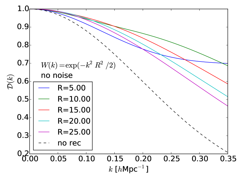
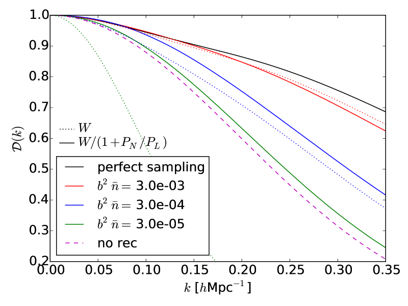
Figure 1: The leading coefficient $\mathcal{D}(k)$ of the reconstructed power spectrum, $P_{\rm rec}(k)={\mathcal{D}}(k)P_{L}(k)+\dots$, for different smoothings and filters. The larger $\mathcal{D}(k)$, the better the reconstruction for the mode $k$. Top: the change in ${\mathcal{D}}(k)$ with changes in the Gaussian smoothing scale $R$. For filtering scale below $\sim 10\,h^{-1}$Mpc, $\mathcal{D}(k)$ is larger at large $k$ and smaller at low $k$ than for $R>10\,h^{-1}$Mpc. Bottom: Holding the smoothing $R=10\,h^{-1}Mpc$, ${\mathcal{D}}(k)$ for different filters and four different choices of isotropic Poisson noise, corresponding to 4 densities. [Densities are quoted in units of $h^{3}\,{\rm Mpc}^{-3}$.] Similar to changing the smoothing scale $R$ above, increasing the noise level (decreasing the density $b^{2}\bar{n}$) can improve reconstruction [increase ${\mathcal{D}}(k)$] for some filters and values of $k$ and degrade reconstruction for others. This can be seen in Fig. 2 below. Also shown is the unreconstructed signal (magenta dashed line) in the absence of noise. Here and hereon, redshift $z=1$ is assumed.

2.3 Reconstruction with noise

In current galaxy redshift surveys targeted at BAO, the number density of tracers is such that noise is relatively insignificant. However this need not be the case in general. When noise is present in the observed field, it will also contribute to the shifted field (White, 2010). Assuming that the signal approaches linearity on large scales, for sufficiently large smoothing the general expression for the shifted field obeys

$$\begin{array}[]{ll}{\bf s}({\bf k})&\simeq-i({\bf k}/k^{2})\ \mathcal{S}({\bf k})\ \left[\delta_{L}({\bf k})+\delta_{N}({\bf k})\right]\;.\end{array}$$ (9)

where we have written the noise contribution $\delta_{N}({\bf k})$ explicitly.

In Eq. 9 the weight, $\mathcal{S}(k)$, applied to the density field is a combination of the usual Gaussian smoothing kernel and a noise-suppression factor,

$$\mathcal{S}({\bf k})=f_{N}\left(P_{L}({\bf k}),P_{N}({\bf k})\right)\,W(k)\;.$$ (10)

Here $P_{L}$ and $P_{N}$ are inputs to the algorithm, taken to be theoretical, linear power spectra estimates for the signal and noise respectively. We shall assume these are the ‘true’ signal and noise spectra, since the procedure can be iterated.

We have not attempted to optimize $f_{N}$. Instead we have chosen it to be a Wiener filter which acts to suppress noise in ${\bf s}$ from modes where $P_{N}$ is as large (or larger) than the cosmological signal.

$$f_{N}\equiv\frac{P_{L}({\bf k})}{P_{L}({\bf k})+P_{N}({\bf k})}=\frac{1}{1+[P_{N}({\bf k})/P_{L}({\bf k})]}\;.$$ (11)

If such a factor $f_{N}$ is not included then a very noisy density field will lead to almost random “shifts” which wash out the structure rather than reconstructing it. A Wiener filter was also suggested by Seo & Hirata (2015, Eq. 17), though they in practice used a Gaussian with a modified smoothing instead.

2.4 Isotropic example

The effects of the noise $P_{N}$ and the filtering $f_{N}$ can be seen clearly in a simplified isotropic example, where $P_{N}({\bf k})=P_{N}(k)$, redshift space distortions are neglected, and the bias $b=1$. In this limit, the leading terms of the reconstructed power spectrum are $P_{\rm rec}({\bf k})=\mathcal{D}({\bf k})P_{L}(k)+\dots$ with

$$\mathcal{D}(k)=e^{-(1/2)k^{2}\Sigma_{ss}^{2}}\left[\mathcal{S}(k)+\left(1-\mathcal{S}(k)\right)e^{-(1/4)k^{2}(\Sigma^{2}-2\Sigma^{2}_{s})}\right]^{2}\;.$$ (12)

Here

$$\Sigma_{ss}^{2} = \frac{1}{3\pi^{2}}\int dp\ \mathcal{S}(p)^{2}\left[P_{L}(p)+P_{N}(p)\right]$$

$$\Sigma_{s}^{2} = \frac{1}{3\pi^{2}}\int dp\ \mathcal{S}(p)P_{L}(p)$$ (13)

and $\Sigma^{2}$ is the unreconstructed damping (Eq. 5). This is equivalent to, but written slightly differently than, previous results (see later). This form isolates both the damping $\Sigma_{ss}^{2}$ remaining after reconstruction (which also contains the full effect of the noise in this approximation) and the damping $\Sigma^{2}$ in the absence of reconstruction. With no filter (i.e., $f_{N}=1$), increasing the noise clearly increases $\Sigma_{ss}^{2}$, increasing the overall damping of the reconstructed linear power spectrum.

Taking $f_{N}$ to be the Wiener filter, $1/(1+P_{N}/P_{L})$, the contributions $\mathcal{S}^{2}[P_{L}+P_{N}]$ in the damping scale in Eq. 13 go to zero when $P_{N}({\bf k})$ is large ($\mathcal{S}P_{L}$ also tends to zero in this limit). The very noisy modes thus do not contribute significantly to $\Sigma_{ss}^{2}$ or to $\Sigma_{s}^{2}$, i.e., to reconstruction. Specifically, $\Sigma_{ss}^{2}$ no longer increases with increasing noise as it would if no filter were applied. In the examples below we shall take the noise to be Poisson shot noise, $P_{N}=b^{-2}\bar{n}^{-1}$, for tracers with number density $\bar{n}$ and linear bias $b$. In fact, we shall typically quote the noise levels in terms of an effective number density.

A filter can not only ensure that noisy modes do not destroy reconstruction for all modes; it also modifies reconstruction for the remaining modes, as does the form and level of noise. These effects can be similar to those due to changing the Gaussian smoothing scale $R$. (Studies changing $R$ include Padmanabhan et al. 2012; Burden et al. 2014; Seo et al. 2015; as mentioned earlier Seo & Hirata (2015) trade a change in $R$ for a filter.) Altering the filter, Gaussian smoothing or noise level does not necessarily have a uniform effect on the reconstruction of different modes: a given change may increase damping for some modes and decrease it for others. In Fig. 1 we show the change in damping, $\mathcal{D}(k)$, when changing the smoothing $R$ (top panel, fixing $f_{N}=1$ by setting $P_{N}=0$) as well as changing the noise level at fixed $R$ (bottom panel). In the latter case we show the results for two filters: $f_{N}=1$ and $f_{N}=1/(1+P_{N}/P_{L})$. Modes at low $k$ and high $k$ have different trends in how well they are reconstructed as the smoothing increases or the filter changes. In particular with a noise dependent filter and smaller $R$ $(R<10\,h^{-1}$Mpc, not shown) increasing noise can increase $\mathcal{D}$ for some low values of $k$. To summarize, the combination of noise, filter and smoothing affects different $k$-modes differently, and increasing noise can sometimes improve reconstruction of a specific $k$-mode. This suggests that a series of filters, each optimized to a specific window and with an optmized shape, could improve reconstruction over what is possible with a single smoothing scale. We shall leave such investigation to a future paper. Henceforth we fix $f_{N}=1/(1+P_{N}({\bf k})/P_{L}({\bf k}))$.

Now we are in a position to describe the effects of missing modes, i.e., modes which are not observed, on reconstruction. First of all, these modes are not present for measuring the power spectrum, which decreases the number of modes which can be averaged over and thus increases the error in a given $k$-bin [perhaps to infinity]. Their absence also weakens the ability to reconstruct the rest of the modes. By treating missing modes as modes with infinite noise in Eq. 12, they can be seen to contribute to the original broadening ($\Sigma^{2}$ is unchanged) but not to the reconstructed factors $\Sigma_{ss}^{2}$ and $\Sigma_{s}^{2}$. Before we explore this further we generalize our treatment to include anisotropic reconstruction and redshift-space distortions.

3 Anisotropic reconstruction

3.1 Formalism

Including redshift-space distortions in our theory, the displacements ${\bf\Psi}$ and ${\bf s}$ are increased in the line-of-sight direction by a factor $1+f$ as noted in section §2.2. The undamped signal is modified from $b^{2}\,P_{L}$ to $(b+f\mu^{2})^{2}P_{L}$, where we have again assumed linear bias $b$. In addition, the noise power spectra appearing in the expressions below are to be interpreted as the raw noise power divided by $[1+\beta\mu^{2}]^{2}$,

$$P_{N}({\bf k})\rightarrow\frac{P_{N}({\bf k})}{[1+\beta\mu^{2}]^{2}}\;,$$ (14)

since we “remove” redshift-space distortions when first computing ${\bf s}$ from our smoothed density field. This additional factor also propagates into the Wiener filter expression and thus $\mathcal{S}({\bf k})$. The noise power, $P_{N}$, may depend on the direction of ${\bf k}$ beyond that given by the $1+\beta\mu^{2}$ term; for example the $21\,$cm wedge corresponds to direction dependent missing modes (i.e., modes with very large noise).

The reconstructed power spectrum thus reads

$$P_{\rm rec}(k,\mu)=(b+f\mu^{2})^{2}\mathcal{D}({\bf k})P_{L}(k)+\cdots$$ (15)

with damping

$$\mathcal{D}({\bf k}) = e^{-(1/2)\{k_{\perp}^{2}\Sigma_{ss,\perp}^{2}+k_{\parallel}^{2}\Sigma_{ss,\parallel}^{2}\}}\left[\frac{1+f\mu^{2}}{b+f\mu^{2}}\,\mathcal{S}({\bf k})+\right.$$

$$\left.\left(1-\frac{1+f\mu^{2}}{b+f\mu^{2}}\,\mathcal{S}({\bf k})\right)e^{-(1/4)\{(k_{\perp}^{2}+(1+f)^{2}k_{\parallel}^{2})\Sigma^{2}-2k_{\perp}^{2}\Sigma_{s,\perp}^{2}-2k_{\parallel}^{2}\Sigma_{s,\parallel}^{2}\}}\right]^{2}\;.$$

The damping terms again depend upon the linear power spectrum and the (now possibly anisotropic) noise, and are given by:

$$\Sigma_{ss,\parallel}^{2} = 2(1+f)^{2}\int\frac{d^{3}p}{(2\pi)^{3}}\frac{p_{\parallel}^{2}}{p^{4}}\ \mathcal{S}^{2}({\bf p})\left[P_{L}({\bf p})+P_{N}({\bf p})\right]$$

$$\Sigma_{ss,\perp}^{2} = \hphantom{2(1+f)^{2}}\int\frac{d^{3}p}{(2\pi)^{3}}\frac{p_{\perp}^{2}}{p^{4}}\ \mathcal{S}^{2}({\bf p})\left[P_{L}({\bf p})+P_{N}({\bf p})\right]$$

$$\Sigma_{s,\parallel}^{2} = 2(1+f)^{2}\int\frac{d^{3}p}{(2\pi)^{3}}\frac{p_{\parallel}^{2}}{p^{4}}\ \mathcal{S}({\bf p})P_{L}({\bf p})$$

$$\Sigma_{s,\perp}^{2} = \hphantom{2(1+f)^{2}}\int\frac{d^{3}p}{(2\pi)^{3}}\frac{p_{\perp}^{2}}{p^{4}}\ \mathcal{S}({\bf p})P_{L}({\bf p})\,$$ (18)

These expressions are equivalent to the more familiar forms

$$\begin{array}[]{lll}\mathcal{D}({\bf k})&=&\mathcal{S}^{2}({\bf k})e^{-(1/2)(k_{\perp}^{2}\Sigma_{ss,\perp}^{2}+k_{\parallel}^{2}\Sigma_{ss,\parallel}^{2})}\\ &+&[1-\mathcal{S}({\bf k})]^{2}e^{-(1/2)(k_{\perp}^{2}\Sigma_{dd,\perp}^{2}+k_{\parallel}^{2}\Sigma_{dd,\parallel}^{2})}\\ &+&2\mathcal{S}({\bf k})[1-\mathcal{S}({\bf k})]e^{-(1/2)(k_{\perp}^{2}\Sigma_{sd,\perp}^{2}+k_{\parallel}^{2}\Sigma_{sd,\parallel}^{2})}\,\,.\end{array}$$ (19)

where we have taken $b=1$ and defined

$$\Sigma_{dd,\parallel}^{2} = 2(1+f)^{2}\int\frac{d^{3}p}{(2\pi)^{3}}\frac{p_{\parallel}^{2}}{p^{4}}\left\{\left[1-\mathcal{S}({\bf p})\right]^{2}P_{L}({\bf p})+\mathcal{S}^{2}({\bf p})P_{N}({\bf p})\right\}$$

$$\Sigma_{dd,\perp}^{2} = \hphantom{2(1+f)^{2}}\int\frac{d^{3}p}{(2\pi)^{3}}\frac{p_{\perp}^{2}}{p^{4}}\left\{\left[1-\mathcal{S}({\bf p})\right]^{2}P_{L}({\bf p})+\mathcal{S}^{2}({\bf p})P_{N}({\bf p})\right\}\,,$$

with $\Sigma^{2}_{sd,\perp}=(1/2)(\Sigma^{2}_{dd,\perp}+\Sigma^{2}_{ss,\perp})$ and $\Sigma^{2}_{sd,\parallel}$ defined similarly. Note that for isotropic $\mathcal{S}$ and $P_{N}$ the parallel components are simply $(1+f)^{2}$ times the perpendicular components and the coefficients of the exponentials become

$$\frac{k^{2}\Sigma^{2}}{2}\left\{(1-\mu^{2})+(1+f)^{2}\mu^{2}\right\}=\frac{k^{2}\Sigma^{2}}{2}\left\{1+f(f+2)\mu^{2}\right\}\quad.$$ (20)

In the appropriate limits these equations then agree with those in Matsubara (2008); White (2010); Carlson, Reid & White (2013); Seo et al. (2015). Note that in the notation of the Appendix of Seo et al. (2015) we have chosen $\kappa=b+f\mu^{2}$ and $\lambda_{d}=\lambda_{s}=f$. It is closest to their “rec-iso” case (in which they choose $\lambda_{s}=0$).

3.2 Example: $21\,$cm wedge

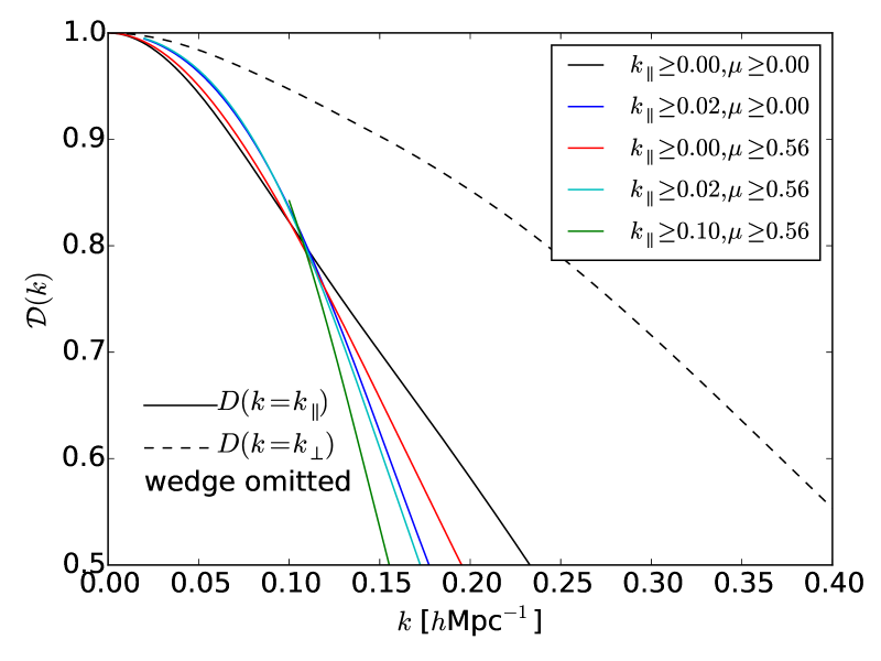
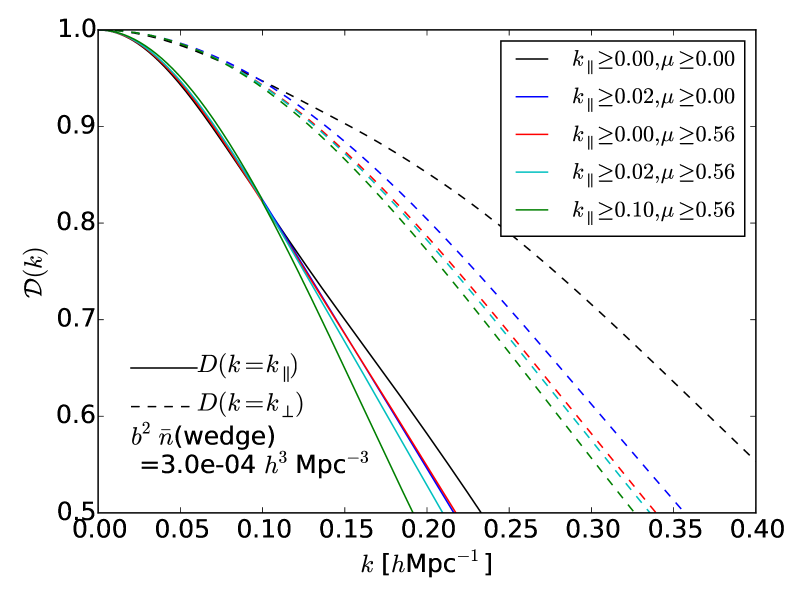
Figure 2: The damping factor, $\mathcal{D}(k)$, for a survey where $21\,$cm modes have $k_{\parallel}$ and $\mu=|k_{\parallel}|/k$ restricted to the ranges shown. The black lines have no missing modes. Colored lines include the effect of the wedge with $\mu_{\rm min}=0.56$ and/or a cut in $k_{\parallel}$; the two lines for the constraints $k_{\parallel}\geq 0.1hMpc^{-1}$, $\mu\geq 0,0.56$ are degenerate. The noise of the $21\,$cm modes, i.e., modes not in the wedge, is taken to be equivalent to $b^{2}\,\bar{n}\simeq 3\times 10^{-3}\,h^{3}{\rm Mpc}^{-3}$ (see text). Two directions are shown: solid lines are along the line-of-sight ($k_{\parallel}=k$, $k_{\perp}=0$) and dashed lines are transverse ($k_{\perp}=k$, $k_{\parallel}=0$). Top: $\mathcal{D}(k)$ for modes which are present (obeying $k_{\parallel}$ and $\mu_{\rm min}$ cut), $P_{N}=\infty$ or $b^{2}\bar{n}\to 0$ for missing modes. Bottom: The same cuts in $k_{\parallel}$, $\mu$, as above, but replacing the missing modes with an ELG survey with number density $3\times 10^{-4}\,h^{3}\,{\rm Mpc}^{-3}$. Note in the top figure that with our approximations a small range of $k_{\parallel}$ is improved when other modes are completely left out of reconstruction, an example of increasing noise increasing $\mathcal{D}(k)$ and suggesting that a different smoothing may help with better recovering those components.

As our motivating example we consider a density field with a noise level and different missing mode scenarios inspired by $21\,$cm experiments. We will take as a representative $21\,$cm noise level that corresponding to the forecast for a CHIME-like experiment in Chang et al. (2008), assuming that thermal noise dominates (see also Seo et al., 2010a; Seo & Hirata, 2015). The CHIME-like noise can be expressed in terms of an effective number density of tracers (of unit bias)

$$\bar{n} = 2.5\times 10^{-3}\,h^{3}{\rm Mpc}^{-3}\left(\frac{1+z}{2.5}\right)^{3/2}$$ (21)

$$\times \left[\frac{\Omega_{\Lambda}(1+z)^{-3}+\Omega_{m}}{0.3}\right]^{-1/2}\left(\frac{\chi}{3.2\,h^{-1}{\rm Gpc}}\right)^{-2}$$

With an eye to using ELG’s as the example of a “helper” tracer we will focus on redshift $z=1$. In this case $\bar{n}\simeq 3\times 10^{-3}\,h^{3}\,{\rm Mpc}^{-3}$.

For missing modes, we consider scenarios where we include only modes with $|k_{\parallel}|>k_{\rm cut}$ which lie outside a “wedge”, $|k_{\parallel}|/k>\mu_{\rm min}$. For definiteness, and because it covers the wide range of opinions in the literature, we consider $k_{\rm cut}=0$, 0.02, $0.1\,h\,{\rm Mpc}^{-1}$. For $\mu_{\rm min}$ the edge of the wedge is given by (e.g., Shaw et al., 2015; Pober, 2015; Seo & Hirata, 2015, and references therein)

$$\frac{k_{\parallel}}{k_{\perp}}\equiv\mathcal{R}=\frac{\chi(z)H(z)}{c(1+z)}=\frac{E(z)}{1+z}\int_{0}^{z}\frac{dz^{\prime}}{E(z^{\prime})}$$ (22)

where $\chi$ is the comoving distance to redshift $z$, $E(z)=H(z)/H_{0}$ and we have assumed a spatially flat Universe. The appropriate prefactor in front of $\mathcal{R}$ and how far into the wedge it is possible to work is a matter of debate – we shall take this value as illustrative though higher values are possible. If the wedge cannot be penetrated then all modes with $|\mu|\equiv|k_{\parallel}|/k<\mu_{\rm min}$

$$\mu_{\rm min}=\frac{\mathcal{R}}{\sqrt{1+\mathcal{R}^{2}}}$$ (23)

are lost. For a $\Lambda$CDM model at $z=1$, and our choice of edge, $\mu_{\rm min}\simeq 0.56$. Thus slightly more than half of all modes would be lost to the wedge at $z=1$. A graphical representation of the modes which are lost (or kept) can be seen in Fig. 4 below.

We show in the top panel of Fig. 2 the change in $\mathcal{D}(k)$, for $k=k_{\parallel}$ or $k=k_{\perp}$ when certain modes are omitted from the reconstruction (the black solid and dashed lines are the comparison case of no missing modes). As already noted by Seo & Hirata (2015), the effect on reconstruction is dramatic. Missing modes thus significantly compromise the ability of a $21\,$cm survey to measure the distance scale.

3.3 Filling in the wedge

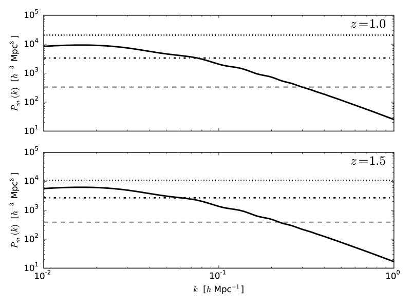
Figure 3: The matter power spectrum, at $z=1$ and 1.5, compared to the QSO shot-noise ($1/b^{2}\bar{n}$; dotted line), the ELG shot-noise (dot-dashed) and the noise expected for a $21\,$cm survey such as CHIME (dashed line). Note that the QSO shot-noise exceeds the cosmological power for all $k$. For $z=1$ we plot the ELG shot-noise for an eBOSS-like sample, assuming $b=1$. At $z=1.5$ we plot the shot-noise assuming constant clustering and DESI-like number densities.

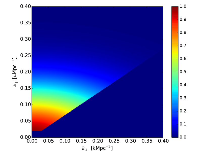
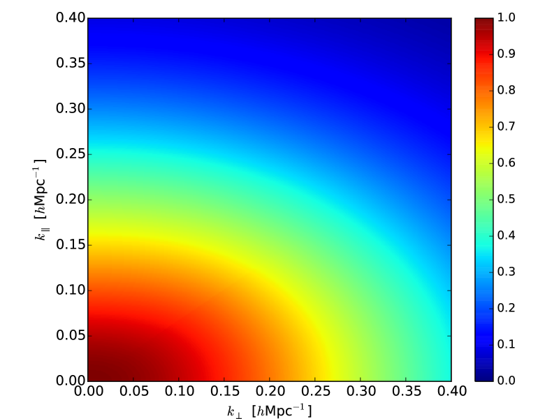
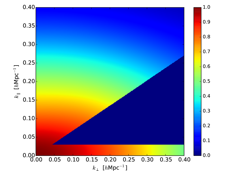
Figure 4: The damping function, $\mathcal{D}({\bf k})$, with $21\,$cm data restricted to $k_{\parallel}\geq 0.02$ and $\mu\geq 0.56$ with an effective density $b^{2}\bar{n}=3\times 10^{-3}\,h^{3}{\rm Mpc}^{-3}$. Top left: no reconstruction. Top right: reconstruction only with $21\,$cm data. Bottom left: reconstruction using ELGs with $b^{2}\bar{n}=3\times 10^{-4}\,h^{3}\,{\rm Mpc}^{-3}$ to fill in the missing modes. Bottom right: reconstruction using a photometric redshift survey with $b^{2}\bar{n}=3\times 10^{-3}\,h^{3}\,{\rm Mpc}^{-3}$ to fill in the modes with $k_{\parallel}<0.03\,h\,{\rm Mpc}^{-1}$. To be able to access such modes requires photo-$z$ precision of $\delta z/(1+z)\sim 0.01$ (see text). Note that in spite of the wedge, non-missing modes along $k_{\perp}$ are much better reconstructed because of redshift space distortions along $k_{\parallel}$.

The top panel of Fig. 2 demonstrates that loss of line-of-sight or wedge modes at low $k$ significantly weakens the ability of a $21\,$cm experiment to constrain the distance scale. However, the modes which are missing are of very long wavelength, near the peak of the CDM power spectrum, and thus can be measured relatively well even by quite sparse tracers. The combined density field then has a noise level which is set by the $21\,$cm survey at high $k$ and the “filler” survey at lower $k$.

As a particular example we shall consider using ELGs as measured for example by eBOSS or DESI. Table 8 of Dawson et al. (2015) lists the ELG number density for the DECam ELG sample as $\sim(1.5-3)\times 10^{-4}\,h^{3}{\rm Mpc}^{-3}$ over the range $0.7<z<1$ and across 1,000 deg². We shall take the upper end of this range as an optimistic example and assume the ELGs are unbiased ($b=1$). This gives the “filler” data a number density an order of magnitude lower than the effective number density for the $21\,$cm data. The amplitudes of the shot noise and cosmological power, as a function of $k$, are compared in Fig. 3.

While in reality one would estimate the density field from the combination of the surveys in an inverse variance manner, and the transition in the noise is likely to be smooth with ${\bf k}$, we shall instead take the noise to be $1/\bar{n}_{21}$ where our $21\,$cm survey has data, sharply transitioning to $1/\bar{n}_{ELG}$ where our $21\,$ survey does not. [Our formalism can handle an arbitrary $P_{N}({\bf k})$.] The lower panel of Fig. 2 shows the improvement that such a survey combination would make in reconstruction – in addition to allowing a measurement of modes inside the foreground-dominated region and so lowering the sample variance for those $k$s.

Fig. 4 shows the full $\mathcal{D}(k_{\perp},k_{\parallel})$ for four cases: no reconstruction, reconstruction using only $21\,$cm data, reconstruction with the addition of the ELGs and reconstruction using a photometric redshift sample (see below). Even missing the modes indicated, a comparison of the top left and right panels shows that reconstruction improves the signal-to-noise of the acoustic signature. However, the improvement that comes from including the missing modes by using ELG data is dramatic, as a comparison of the bottom left and top right panels shows. We discuss the lower right panel below.

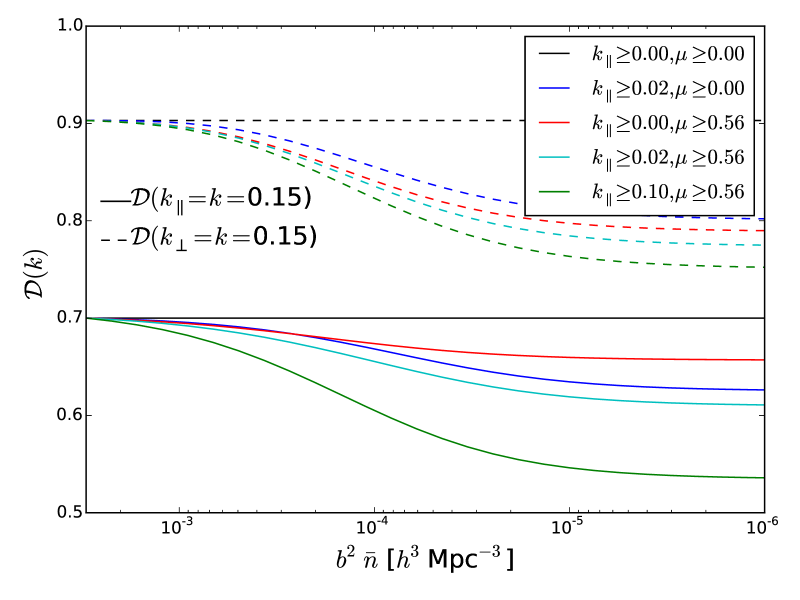
Figure 5: The damping function at $k=0.15\,h\,{\rm Mpc}^{-1}$ as a function of ELG density for different wedge shapes (as indicated in the figure). Solid lines show $\mathcal{D}$ for $k_{\parallel}=k=0.15\,h\,{\rm Mpc}^{-1}$ while dashed lines show $k_{\perp}=k=0.15\,h\,{\rm Mpc}^{-1}$. The small density, i.e., large noise, limits asymptotically reach the $\mathcal{D}(k)$ where only the $21\,$cm measurements are available. (If a mode is missing entirely when only $21\,$cm measurements are available, then it will not contribute before or after reconstruction.) In spite of the wedge, modes along $k_{\perp}$ are much better reconstructed because of redshift space distortions along $k_{\parallel}$. The line for the constraint $k_{\parallel}\geq 0.1\,h\,{\rm Mpc}^{-1}$ is the same for $\mu\geq 0,0.56$.

We find that the combination of experiments does better than either does alone. The improvement over a $21\,$cm experiment which cannot measure some modes is demonstrated above. Although we do not show it here, the combination of the $21\,$cm data and the ELGs provides slightly better reconstruction than can be obtained with a survey of only ELGs (unless their number density can be increased by an order of magnitude). The damping scales, $\Sigma_{s}$ and $\Sigma_{ss}$, are common to all modes and benefit from the regions of $k$-space with lower noise. For our fiducial ELG number density the improvement is not dramatic since the noise is subdominant to the signal power for a broad range of $k$, however the situation changes if such high number densities cannot easily be obtained over the desired redshift range.

To further explore the parameter space, Fig. 5 shows the damping function along or transverse to the line of sight (with $k=0.15\,h\,{\rm Mpc}^{-1}$) as a function of tracer noise (specifically $b^{2}\bar{n}$) for different choices of the missing modes. One can see that once the number density of the tracer has $b^{2}\bar{n}\simeq 10^{-4}\,h^{3}\,{\rm Mpc}^{-3}$ or larger it is able to compensate for the modes missed by the $21\,$cm survey and improve the performance of reconstruction. This characteristic number density is given by the cosmological power ($P_{L}$) at the scales where the $21\,$cm survey is missing modes, which is close to the peak of the power spectrum.

So far our discussion has assumed that the “filler” sample comes from a spectroscopic survey. However, if only the low $k$ modes are needed, samples and surveys with high-precision photometric redshifts could be used instead. The lower right panel of Fig. 4 shows an optimistic case where a photometric redshift survey can fill in all of the modes with $k_{\parallel}<0.03\,h\,{\rm Mpc}^{-1}$. (This includes some modes already obtained from $21\,$cm outside the wedge, but adds information inside the wedge.) Translating a redshift uncertainty of $\delta z$ into a comoving distance uncertainty of $\delta\chi=[c/H(z)]\delta z$, to probe $k_{\parallel}=0.03\,h\,{\rm Mpc}^{-1}$ requires $\delta z/(1+z)<0.01$ at $z=1$. Such photo-$z$ precision is in principle achievable, given enough filters. As shown in Fig. 4 lower right, recovering $k_{\parallel}<0.03\,h\,{\rm Mpc}^{-1}$ (for all $k_{\perp}$) can have a large impact on reconstruction. Conversely, if only $k_{\parallel}<0.01\,h\,{\rm Mpc}^{-1}$ can be recovered then the gain is minimal.

4 Discussion

The study of large-scale structure has taught us a great deal about the Universe in which we live and provides tight constraints on fundamental physics. One of the key observables in large-scale structure are the so-called BAO, which provide a standard ruler enabling the measurement of the expansion history of the Universe with low systematics and high precision. The BAO signal is degraded by non-linear evolution, but the degradation can to some degree be overcome by density field reconstruction.

While $21\,$cm experiments can in principle measure large-scale structure efficiently at very high redshifts, where galaxy redshift surveys become increasingly expensive, they may suffer from large foreground contamination in a “wedge” in $k$-space. The modes lost due to foregrounds have an impact on BAO measurements but an even larger impact upon reconstruction (as recently emphasized by Seo & Hirata, 2015). In this paper we have demonstrated, using an analytic model based on low-order Lagrangian perturbation theory, that even a relatively sparse tracer of the density field can “fill in” the missing modes. The combined data can be more powerful than either of its parts: reaping the benefits of full $k$-coverage and low shot-noise. This allows density field reconstruction and tight measurements at smaller scales, which can be especially useful at higher $z$.

We have presented formulae for the efficacy of reconstruction in the case of biased tracers of the density field, including redshift-space distortions, anisotropic noise and noise-filtering during reconstruction. The missing modes can be modeled as infinite noise, while the effects of having two different samples can be modeled via anisotropic noise. These extend the formulae in the literature, but agree with those formulae in the appropriate limits. We find that the details of how BAO are predicted to be damped in Lagrangian perturbation theory depend upon the shape of the filter applied to estimate the shift field. If this finding holds up in simulations, it opens the possibility of “shaping” the filter to improve the performance of reconstruction.

While even a very noisy tracer of the density field can be used to measure the power spectrum if enough modes can be averaged together, our intuition tells us that reconstruction — which depends on the 3D density field and not just its power spectrum — requires noise per $k$-mode less than the cosmological signal. Our calculation quantifies and supports this intuition, and we show that to measure the low-$k$ modes missed by a $21\,$cm survey tracers with $b^{2}\bar{n}\sim 10^{-3}-10^{-4}\,h^{3}\,{\rm Mpc}^{-3}$ are required.

Of the existing surveys that cover large cosmological volumes at high redshift, the QSO surveys are currently too sparse to be of significant benefit. An increase in number density, however, would lead to improved performance. Some of the low $k_{\parallel}$ modes could, in principle, be filled in with a photometric sample with excellent photometric redshifts (obtained, perhaps, using multiple medium bands). In the near term the most promising tracer, in the redshift range $z>1$ where most future $21\,$cm surveys will be operating, are ELGs such as will be measured by eBOSS or DESI. If eBOSS can achieve its forecast number densities it would significantly improve reconstruction for $21\,$cm surveys which overlap in volume. In the future even the higher $z$ tail of the DESI ELG sample (with its higher bias) would be beneficial to $21\,$cm surveys which are unable to work deep into the foreground wedge.

We would like to thank Marcel Schmittfull for helpful conversations on acoustic oscillations and reconstruction, and Josh Dillon, Daniel Eisenstein, Marcel Schmittfull, Uros Seljak and Hee-Jong Seo for helpful feedback on the draft, and the anonymous referee for additional helpful suggestions. This work was begun at the Aspen Center for Physics, which is supported by National Science Foundation grant PHY-1066293. We thank the Center for its hospitality. T.-C.C. acknowledges support from MoST grant 103-2112-M-001-002-MY3. This work made extensive use of the NASA Astrophysics Data System and of the astro-ph preprint archive at arXiv.org.

Appendix A Deriving the damping

Starting with the expression for $\delta({\bf k})$ in the text [Eq. 2] we can write [setting bias $b=1$, or $F[\lambda]\propto\delta^{(D)}(\lambda)$]

$$\left\langle\delta({\bf k}_{1})\delta^{\star}({\bf k}_{2})\right\rangle=\left\langle\int d{\bf q}_{1}\,d{\bf q}_{2}e^{-i{\bf k}_{1}\cdot{\bf q}_{1}}e^{i{\bf k}_{2}\cdot{\bf q}_{2}}[e^{-i{\bf k}_{1}\cdot{\bf\Psi}({\bf q}_{1})}e^{i{\bf k}_{2}\cdot{\bf\Psi}({\bf q}_{2})}-1]\right\rangle\quad.$$ (24)

Employing the cumulant theorem for a Gaussian variable ($\langle\exp[iX]\rangle=\exp[-(1/2)\langle X^{2}\rangle]$), making a change of variables $d{\bf q}_{1}\,d{\bf q}_{2}\to d\mathbf{Q}\,d{\bf q}$ with ${\bf q}={\bf q}_{1}-{\bf q}_{2}$ and $2\mathbf{Q}={\bf q}_{1}+{\bf q}_{2}$ and using translational symmetry we have

$$P(k)=\int d^{3}q\ e^{-i{\bf k}\cdot{\bf q}}\exp\left[-k_{i}k_{j}\left\{\xi_{ij}(\mathbf{0})-\xi_{ij}({\bf q})\right\}\right]$$ (25)

where we have defined $\xi_{ij}({\bf q})=\left\langle\Psi_{i}({\bf q})\Psi_{j}(\mathbf{0})\right\rangle$ and assumed ${\bf k}\neq 0$. Extracting the $q$-independent piece of the integral and expanding the exponential gives

$$P(k)=\exp\left[-k_{i}k_{j}\xi_{ij}(\mathbf{0})\right]\int d^{3}q\ e^{-i{\bf k}\cdot{\bf q}}\left[k_{i}k_{j}\xi_{ij}({\bf q})+\cdots\right]$$ (26)

The Fourier transform of the $k_{i}k_{j}\xi_{ij}({\bf q})$ term can easily be shown to be $P_{L}(k)$ to lowest order,

$$\int d^{3}q\ e^{-i{\bf k}\cdot{\bf q}}k_{i}k_{j}\xi_{ij}({\bf q}) = k_{i}k_{j}\int d^{3}q\ e^{-i{\bf k}\cdot{\bf q}}\int\frac{d^{3}p}{(2\pi)^{3}}$$

$$\times e^{i{\bf p}\cdot{\bf q}}\frac{p_{i}p_{j}}{p^{4}}P_{L}(p)$$

$$= k_{i}k_{j}\int\frac{d^{3}p}{(2\pi)^{3}}\frac{p_{i}p_{j}}{p^{4}}P_{L}(p)$$

$$\times \ (2\pi)^{3}\delta({\bf p}-{\bf k})$$ (28)

$$= P_{L}(k)$$ (29)

while the exponential is the source of the damping term of the BAO features (or the broadening of the acoustic peak in the correlation function)

$$\xi_{ij}(\mathbf{0})=\int\frac{d^{3}k}{(2\pi)^{3}}\frac{k_{i}k_{j}}{k^{4}}P_{L}(k)=\frac{\delta_{ij}}{3}\int\frac{dk}{2\pi^{2}}\ P_{L}(k)\quad.$$ (30)

Appendix B Reconstruction in Eulerian perturbation theory

Most of the reconstruction literature either prescribes its implementation on a data set or interprets this implementation within Lagrangian perturbation theory. However, recently Schmittfull et al. (2015) developed a theory of reconstruction based on Eulerian perturbation theory and introduced several new reconstruction schemes. One advantage of the Eulerian formulation, especially in the present context, is that it is naturally expressed in terms of the Fourier space density fields which are measured by $21\,$cm experiments. A disadvantage of the Eulerian schemes is the increased difficulty of including redshift-space distortions. In this appendix we consider the impact of missing modes upon reconstruction in the Eulerian scheme to build intuition about their impact. We restrict ourselves to real-space measures, set the bias to $1$ and the noise to zero for modes which have measurements. This preserves the main features of the problem while simplifying the presentation.

Heuristically, reconstruction works by “undoing” some of the nonlinear time evolution which decreases and shifts the BAO peak. For Eulerian reconstruction, Schmittfull et al. (2015) approximate the initial density field by Taylor expanding the observed field at late times, specifically subtracting $\Delta t\,\dot{\delta}$. Using the continuity equation to express $\dot{\delta}$ in terms of the divergence of $(1+\delta)v$, and with an appropriate choice of $\Delta t$ some algebra gives (Schmittfull et al., 2015)

$$\delta_{r}({\bf x})=\delta_{\rm obs}({\bf x})-{\bf s}({\bf x})\cdot\vec{\nabla}\delta_{\rm obs}({\bf x})-\delta_{\rm obs}({\bf x})\delta_{R}({\bf x})\;.$$ (31)

Here ${{\bf s}}({\bf k})=-i{\bf k}/k^{2}\ \delta_{\rm obs}({\bf k})W(k)$ is the shift vector and $\delta_{R}({\bf k})=\delta_{\rm obs}({\bf k})W(k)$, with a smoothing kernel $W(k)$ (usually a Gaussian). In Fourier space, this becomes

$$\delta_{r}({\bf k})=\delta_{\rm obs}({\bf k})-\int\frac{d^{3}p}{(2\pi)^{3}}\mathcal{K}({\bf k}-\mathbf{p},\mathbf{p})\delta_{\rm obs}({\bf k}-\mathbf{p})\delta_{\rm obs}(\mathbf{p})$$ (32)

where by changing the kernel, $\mathcal{K}$, we can now describe more general reconstruction methods.

The reconstructed power spectrum is $P_{\rm rec}(k)\propto\langle\left|\delta_{r}^{2}\right|\rangle$ as before. The leading contribution to enhancing the BAO features, i.e., to reconstruction, was found by Schmittfull et al. (2015) to be (their Eq. 69):

$$\left\langle\Delta^{(3)}({\bf k})\delta_{L}({\bf k}^{\prime})\right\rangle=3(2\pi)^{3}\delta({\bf k}+{\bf k}^{\prime})P_{\rm lin}(k)\int\frac{d^{3}k_{1}}{(2\pi)^{3}}D_{3}({\bf k}_{1},-{\bf k}_{1},{\bf k})P_{L}(k_{1})\;.$$ (33)

This 3-point term can be seen to explicitly enhance the oscillations over those in $P_{\rm obs}(k)$, restoring some of the signal that is damped by non-linear evolution and bringing the result closer to $P_{L}(k)$.

In more detail,

$$D_{3}({\bf k_{1},k_{2},k_{3}})=-\frac{2}{3}[\mathcal{K}({\bf k}_{1},{\bf k}_{2}+{\bf k}_{3})F_{2}({\bf k}_{2},{\bf k}_{3})+\;{\rm cyclic}]\;,$$ (34)

where

$$F_{2}({\bf k}_{1},{\bf k}_{2})=\frac{5}{7}+\frac{1}{2}\left(\frac{k_{1}}{k_{2}}+\frac{k_{2}}{k_{1}}\right)\hat{k}_{1}\cdot\hat{k}_{2}+\frac{2}{7}\left(\hat{k}_{1}\cdot\hat{k}_{2}\right)^{2}\;.$$ (35)

is the usual perturbation theory kernel. For the Schmittfull et al. (2015) EGS reconstruction method

$${\mathcal{K}}({\bf k}_{1},{\bf k}_{2})=\frac{1}{2}\left[W(k_{1})+W(k_{2})\right]+W(k_{1})\frac{{\bf k}_{1}\cdot{\bf k}_{2}}{k_{1}^{2}}\;,$$ (36)

and, defining $\mu=\hat{k}_{1}\cdot\hat{k}$,

$$D_{3}({\bf k_{1},-k_{1},k}) = \frac{2}{3}\left[-\frac{1}{2}(W({\bf k}+{\bf k}_{1})+W({\bf k}-{\bf k}_{1}))\right.\left[\frac{5}{7}+\frac{2}{7}\mu^{2}\right]$$ (37)

$$-\frac{1}{4}\left[W({\bf k}+{\bf k}_{1})-W({\bf k}-{\bf k}_{1})\right]\mu\left[\frac{k}{k_{1}}+\frac{k_{1}}{k}\right]$$

$$\left.+W(k_{1})\left[\frac{5}{7}+\mu^{2}\left(\frac{9}{7}+\frac{k^{2}}{k_{1}^{2}}\right)\right]\right]\;.$$

Fig. 6 shows the contribution of different modes to $D_{3}({\bf k}_{1},-{\bf k}_{1},{\bf k})P_{L}(k_{1})k_{1,\perp}$. The modes which contribute most to $D_{3}$ contribute the most to restoring the BAO signal, i.e., to reconstruction. Two different modes with $k=0.15\,h\,{\rm Mpc}^{-1}$ are shown, along the $\hat{k}_{1,z}$ and $\hat{k}_{1,x}$ axes (the latter shown in the $\hat{k}_{1,z}-\hat{k}_{1,x}$ plane). Equal area in this plot gets equal weight in the integral, so that the relative importance of different modes can be read off more easily.

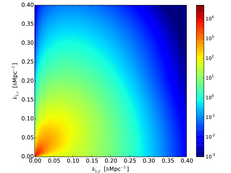
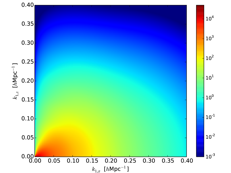
Figure 6: Two slices in the $\hat{k}_{1,x},\hat{k}_{1,z}$ plane of the integrand $D_{3}({\bf k_{1},-k_{1},k})P_{L}(k_{1})k_{1,\perp}$ in Eq. 33. Its integral is the dominant contribution in reconstruction of the linear power spectrum $P_{L}({\bf k})$, as noted in Schmittfull et al. (2015). The top figure has the contribution for observed mode ${\bf k}=0.15\hat{k}_{\parallel}=0.15\hat{k}_{z}$, and the bottom figure corresponds to ${\bf k}=0.15\hat{k}_{x}$. The measure of integration is $dk_{\parallel}dk_{\perp}=dk_{\parallel}dk_{x}$ in this plane, thus area is a measure of the size of the contribution to reconstruction. Note that the color scale is logarithmic in this plot, unlike the earlier plots.

As before, if an interferometer does not measure a given ${\bf k}_{1}$ mode, it will not contribute to $D_{3}$ but it will contribute to the damping of the signal in $P_{\rm obs}$. A simple way to see the effect of missing modes to reconstruction of a mode ${\bf k}$ is to ask what impact removing contributions from ${\bf k}_{1}$ and ${\bf k}\pm{\bf k}_{1}$ would have. Visually it is clear that the modes where the color scale is red or orange contribute the majority of $D_{3}$, so losing these modes has the largest detrimental effect on reconstruction. This agrees with our the intuition obtained from the Lagrangian theory exposition in the main text.

References

- Ali & Bharadwaj (2014) Ali S. S., Bharadwaj S., 2014, Journal of Astrophysics and Astronomy, 35, 157
- Anderson et al. (2014) Anderson L. et al., 2014, MNRAS, 441, 24
- Ansari et al. (2012) Ansari R., Campagne J.-E., Colom P., Magneville C., Martin J.-M., Moniez M., Rich J., Yèche C., 2012, Comptes Rendus Physique, 13, 46
- Bharadwaj (1996) Bharadwaj S., 1996, ApJ, 460, 28
- Burden et al. (2014) Burden A., Percival W. J., Manera M., Cuesta A. J., Vargas Magana M., Ho S., 2014, MNRAS, 445, 3152
- Busca et al. (2013) Busca N. G. et al., 2013, A&A, 552, A96
- Carlson, Reid & White (2013) Carlson J., Reid B., White M., 2013, MNRAS, 429, 1674
- Chang et al. (2010) Chang T.-C., Pen U.-L., Bandura K., Peterson J. B., 2010, Nature, 466, 463
- Chang et al. (2008) Chang T.-C., Pen U.-L., Peterson J. B., McDonald P., 2008, Physical Review Letters, 100, 091303
- Crocce & Scoccimarro (2008) Crocce M., Scoccimarro R., 2008, Phys. Rev. D, 77, 023533
- Croom et al. (2005) Croom S. M. et al., 2005, MNRAS, 356, 415
- Datta, Bowman & Carilli (2010) Datta A., Bowman J. D., Carilli C. L., 2010, ApJ, 724, 526
- Dawson et al. (2015) Dawson K. S. et al., 2015, ArXiv e-prints
- Delubac et al. (2015) Delubac T. et al., 2015, A&A, 574, A59
- Eisenstein et al. (2007) Eisenstein D. J., Seo H.-J., Sirko E., Spergel D. N., 2007, ApJ, 664, 675
- Eisenstein, Seo & White (2007) Eisenstein D. J., Seo H.-J., White M., 2007, ApJ, 664, 660
- Font-Ribera et al. (2014) Font-Ribera A. et al., 2014, JCAP, 5, 27
- Furlanetto, Oh & Briggs (2006) Furlanetto S. R., Oh S. P., Briggs F. H., 2006, Physics Reports, 433, 181
- Kirkby et al. (2013) Kirkby D. et al., 2013, JCAP, 3, 24
- Liu, Parsons & Trott (2014) Liu A., Parsons A. R., Trott C. M., 2014, Phys. Rev. D, 90, 023019
- Matsubara (2008) Matsubara T., 2008, Phys. Rev. D, 77, 063530
- McCullagh & Szalay (2012) McCullagh N., Szalay A. S., 2012, ApJ, 752, 21
- Meiksin, White & Peacock (1999) Meiksin A., White M., Peacock J. A., 1999, MNRAS, 304, 851
- Morales et al. (2012) Morales M. F., Hazelton B., Sullivan I., Beardsley A., 2012, ApJ, 752, 137
- Myers et al. (2015) Myers A. D. et al., 2015, ArXiv e-prints
- Nan et al. (2011) Nan R. et al., 2011, International Journal of Modern Physics D, 20, 989
- Noh, White & Padmanabhan (2009) Noh Y., White M., Padmanabhan N., 2009, Phys. Rev. D, 80, 123501
- Olive et al. (2014) Olive K. A., et al., 2014, Chin. Phys., C38, 090001
- Padmanabhan & White (2009) Padmanabhan N., White M., 2009, Phys. Rev. D, 80, 063508
- Padmanabhan, White & Cohn (2009) Padmanabhan N., White M., Cohn J. D., 2009, Phys. Rev. D, 79, 063523
- Padmanabhan et al. (2012) Padmanabhan N., Xu X., Eisenstein D. J., Scalzo R., Cuesta A. J., Mehta K. T., Kazin E., 2012, MNRAS, 427, 2132
- Parsons et al. (2012) Parsons A. R., Pober J. C., Aguirre J. E., Carilli C. L., Jacobs D. C., Moore D. F., 2012, ApJ, 756, 165
- Pober (2015) Pober J. C., 2015, MNRAS, 447, 1705
- Pober et al. (2013) Pober J. C. et al., 2013, AJ, 145, 65
- Schmittfull et al. (2015) Schmittfull M., Feng Y., Beutler F., Sherwin B., Yat Chu M., 2015, ArXiv e-prints
- Seo et al. (2015) Seo H.-J., Beutler F., Ross A. J., Saito S., 2015, ArXiv e-prints
- Seo et al. (2010a) Seo H.-J., Dodelson S., Marriner J., Mcginnis D., Stebbins A., Stoughton C., Vallinotto A., 2010a, ApJ, 721, 164
- Seo et al. (2010b) Seo H.-J. et al., 2010b, ApJ, 720, 1650
- Seo & Hirata (2015) Seo H.-J., Hirata C. M., 2015, ArXiv e-prints
- Shaw et al. (2014) Shaw J. R., Sigurdson K., Pen U.-L., Stebbins A., Sitwell M., 2014, ApJ, 781, 57
- Shaw et al. (2015) Shaw J. R., Sigurdson K., Sitwell M., Stebbins A., Pen U.-L., 2015, Phys. Rev. D, 91, 083514
- Sherwin & Zaldarriaga (2012) Sherwin B. D., Zaldarriaga M., 2012, Phys. Rev. D, 85, 103523
- Slosar et al. (2013) Slosar A. et al., 2013, JCAP, 4, 26
- Tassev & Zaldarriaga (2012a) Tassev S., Zaldarriaga M., 2012a, JCAP, 4, 13
- Tassev & Zaldarriaga (2012b) Tassev S., Zaldarriaga M., 2012b, JCAP, 10, 6
- Taylor & Hamilton (1996) Taylor A. N., Hamilton A. J. S., 1996, MNRAS, 282, 767
- Tojeiro et al. (2014) Tojeiro R. et al., 2014, MNRAS, 440, 2222
- Vargas-Magaña et al. (2014) Vargas-Magaña M. et al., 2014, MNRAS, 445, 2
- Vedantham, Udaya Shankar & Subrahmanyan (2012) Vedantham H., Udaya Shankar N., Subrahmanyan R., 2012, ApJ, 745, 176
- White (2010) White M., 2010, ArXiv e-prints
- White (2015) White M., 2015, MNRAS, 450, 3822
- Xu et al. (2013) Xu X., Cuesta A. J., Padmanabhan N., Eisenstein D. J., McBride C. K., 2013, MNRAS, 431, 2834
- Zel’dovich (1970) Zel’dovich Y. B., 1970, A&A, 5, 84
- Zhu et al. (2015) Zhu H.-M., Pen U.-L., Yu Y., Er X., Chen X., 2015, ArXiv e-prints