Nonlocal and multipoint boundary value problems
for linear evolution equations

Abstract

We derive the solution representation for a large class of nonlocal boundary value problems for linear evolution PDEs with constant coefficients in one space variable. The prototypical such PDE is the heat equation, for which problems of this form model physical phenomena in chemistry and for which we formulate and prove a full result. We also consider the third order case, which is much less studied and has been shown by the authors to have very different structural properties in general.

The nonlocal conditions we consider can be reformulated as multipoint conditions, and then an explicit representation for the solution of the problem is obtained by an application of the Fokas transform method. The analysis is carried out under the assumption that the problem being solved is well posed, i.e. that it admits a unique solution. For the second order case, we also give criteria that guarantee well-posedness.

1 Introduction

In a variety of applications of PDE models, classical boundary conditions imposed at the boundary of the domain are not representative of the particular phenomenon, and it is necessary to consider nonlocal boundary conditions. A particular example of such nonlocal conditions are multipoint conditions relating the value of the solution at the boundary points with the values at some interior points. A simple example of this is given in [3], where motivation from physical applications, particularly in chemistry, can also be found. Early work on three-point boundary conditions was done in [18, 23], though these works focus on the analysis and proving existence of a solution of possibly nonlinear ODEs of second order. Indeed, most existing results are limited to the second order case, either linear or nonlinear, although some third order results are presented in [24]. Related important developments have focused on solving PDEs, linear and nonlinear, on networks, including linear networks [31].

A wide class of more general nonlocal problems can be shown to be equivalent to multipoint problems, see section 2.1 below. This class includes problems in which one or more boundary conditions is replaced by a nonlocal condition specifying the integral of the solution on a certain subinterval of the spatial domain. For a heat conduction problem, this may represent conservation of the internal energy on a subinterval of the spatial domain [5]. For a diffusion problem, the integral may represent the total mass of a certain chemical within a given region, which could be easily measured using a photometer [4]. A number of other applications for similar second order problems are described in [8, 9].

In this paper, we make use of the Fokas transform (also known in the literature as the unified transform) to give a general solution to multipoint boundary value problems for linear PDEs of arbitrary order of the form

$$q_{t}+a(-i\partial_{x})^{n}q=0,\qquad x\in(0,1),\quad t>0.$$ (1.1)

We assume here that $n\geqslant 2$ (the special case $n=1$ will be considered elsewhere). The coefficient $a$ is assumed to satisfy the restriction (2.4) below, which essentially ensures that the Cauchy initial value problem for the PDE is well posed on $t>0$. The choice of equations with only the term of highest order spatial derivative may seem special. However, the analysis of these particular PDEs captures the essential features of the solution also for the case of constant coefficient linear PDEs with lower order terms, see for example [26] for a full discussion and justification of this claim.

A typical multipoint boundary value problem is the one studied in [3]:

Find the function $q(x,t)$, $x\in(0,1)$, $t>0$ such that $q_{t}=q_{xx}$, and $q$ satisfies the given (sufficiently smooth) initial condition $q(x,0)=q_{0}(x)$ and the additional conditions

$$q(0,t)=c_{0}\,q\left(\frac{1}{2},t\right)+d_{0}(t)\quad{\rm and}\quad q(1,t)=c_{1}\,q\left(\frac{1}{2},t\right)+d_{1}(t).$$ (1.2)

We give a more comprehensive solution than provided in previous papers to a more general form of this problem, for a PDE of arbitrary order and multipoint conditions linking an arbitrary number of interior points $\eta_{1},\ldots,\eta_{m-1}\in(0,1)$, with $\eta_{0}=0$ and $\eta_{m}=1$. Our most complete result is theorem 5.4 for the heat equation, but the majority of the analysis is carried out in much greater generality. In particular, we prove the following theorem.

Theorem 1.1.

Suppose $q(x,t)$ is the solution of initial-$(m+1)$ point value problem of order $n$ defined below in (2.2).

Then $q(x,t)$ admits the integral representation (see equation (4.6))

$$2\pi q(x,t)=\int_{-\infty}^{\infty}{\rm e}^{i\lambda x-a\lambda^{n}t}\hat{q}_{0}(\lambda)\,\mathrm{d}\lambda-\int_{\partial D_{R}\cap\mathbb{C}^{+}}{\rm e}^{i\lambda x-a\lambda^{n}t}\sum_{k=0}^{n-1}f_{k}^{0}(\lambda;T)\,\mathrm{d}\lambda\\ -\int_{\partial D_{R}\cap\mathbb{C}^{-}}{\rm e}^{i\lambda(x-1)-a\lambda^{n}t}\sum_{k=0}^{n-1}f_{k}^{m}(\lambda;T)\,\mathrm{d}\lambda.$$

In the above expression, $\hat{q}_{0}$ is defined by (3.5) and $D_{R}$ is given by (3.7). The terms involving the functions $f_{k}^{r}$ are obtained as the solution of linear system (4.12). In the particular case $n=2$ (respectively, $n=3$), the solution of this system is provided by lemma 5.1 (respectively, lemma 6.1).

The paper is organised as follows. In section 2, we formulate the general multipoint condition, and we show how a large class of nonlocal conditions can be reformulated as multipoint conditions, so fall within the scope of the present work. In section 3, we give a concise introduction to the Fokas transform in general, and then in section 4 we apply it to the general multipoint boundary problem formulated in section 2. By the end of section 4, the first two claims of theorem 1.1 are established. In sections 5 and 6, we study in detail the second and third order case respectively, both in general and for specific examples. In particular, in section 5 we state and prove theorem 5.4. The appendices contain proofs of the lemmata that conclude theorem 1.1.

2 Formulation of the problem

Let $m,n\in\mathbb{N}$ be independent,

$$0=\eta_{0}<\eta_{1}<\eta_{2}<\ldots<\eta_{m}=1,$$ (2.1)

and

$$b_{k\hskip 1.42262ptj}^{r}\in\mathbb{C}\quad\mbox{for }k,j\in\{0,\ldots,n-1\},\;\;r\in\{0,\ldots,m\}.$$

Consider the initial-multipoint value problem

$$[\partial_{t}+a(-i\partial_{x})^{n}]q(x,t) =0 (x,t) \in(0,1)\times(0,T),$$ (2.2a)

$$q(x,0) =q_{0}(x) x \in[0,1],$$ (2.2b)

$$\sum_{k=0}^{n-1}\sum_{r=0}^{m}b_{k\hskip 1.42262ptj}^{r}\partial_{x}^{k}q(\eta_{r},t) =g_{j}(t) t \in[0,T],\quad j\in\{0,1,\ldots,n-1\},$$ (2.2c)

where we assume $g_{j}\in C^{\infty}[0,T]$ with $T>0$ a fixed constant, and that the initial datum is compatible with the multipoint data in the sense that

$$q_{0}\in C^{n}[0,1]\quad{\rm and}\quad\sum_{k=0}^{n-1}\sum_{r=0}^{m}b_{k\hskip 1.42262ptj}^{r}\partial_{x}^{k}q_{0}(\eta_{r})=g_{j}(0).$$ (2.3)

We always assume that the coefficient $a$ satisfies

$$a\in\begin{cases}\{e^{i\theta}:\theta\in[0,\pi]\}&\mbox{if }n\mbox{ even,}\\ \{i,-i\}&\mbox{if }n\mbox{ odd.}\end{cases}$$ (2.4)

Assuming that a solution $q\in C^{n}(0,1)$ exists and is unique, we give a representation of this solution by an application of the Fokas transform approach. The Fokas transform is an integral transform flexible enough to allow us to derive a general and effective representation of the solution of any such boundary value problem.

The explicit solution representation we derive can be used to justify a posteriori the existence and uniqueness assumption.

2.1 Nonlocal boundary conditions

The multipoint boundary condition (2.2c) is actually a rather general nonlocal condition. We first illustrate this observation with an example.

Consider the initial-nonlocal value problem

$$[\partial_{t}-\partial_{x}^{2}]q(x,t) =0 (x,t) \in(0,1)\times(0,T),$$ (2.5a)

$$q(x,0) =q_{0}(x) x \in[0,1],$$ (2.5b)

$$\int_{0}^{\frac{1}{2}}q(x,t)\,\mathrm{d}x =0 t \in[0,T],$$ (2.5c)

$$\int_{\frac{1}{2}}^{1}(1-x)q(x,t)\,\mathrm{d}x =0 t \in[0,T],$$ (2.5d)

which can be seen as a generalization of a problem studied by Mantzavinos [14]. We claim that problem (2.5) is equivalent to an initial multipoint value problem belonging to class (2.2). To wit, differentiate both nonlocal conditions (2.5c)–(2.5d) with respect to $t$, and apply (2.5a), to obtain

$$\int_{0}^{\frac{1}{2}}\partial_{x}^{2}q(x,t)\,\mathrm{d}x=0,\qquad\int_{\frac{1}{2}}^{1}(1-x)\partial_{x}^{2}q(x,t)\,\mathrm{d}x=0,$$ (2.6)

respectively. Integrating (by parts in the latter), one obtains the multipoint conditions

$$\partial_{x}q\left(\frac{1}{2},t\right)-\partial_{x}q(0,t)=0 t \in[0,T],$$ (2.7a)

$$\frac{1}{2}\partial_{x}q\left(\frac{1}{2},t\right)-q(1,t)+q\left(\frac{1}{2},t\right)=0 t \in[0,T].$$ (2.7b)

In general, suppose $J\in\{-1,\ldots,n-1\}$, and consider problem (2.2), but with (2.2c) replaced by the multipoint and nonlocal conditions

$$\sum_{k=0}^{n-1}\sum_{r=0}^{m}b_{k\hskip 1.42262ptj}^{r}\partial_{x}^{k}q(\eta_{r},t) =g_{j}(t) t \in[0,T],\quad j\in\{0,1,\ldots,J\},$$ (2.8a)

$$\sum_{k=0}^{n-1}\sum_{r=1}^{m}\int_{\eta_{r-1}}^{\eta_{r}}b_{k\hskip 1.42262ptj}^{r}x^{k}q(x,t)\,\mathrm{d}x =g_{j}(t) t \in[0,T],\quad j\in\{J+1,\ldots,n-1\}.$$ (2.8b)

Proposition 2.1.

The initial-nonlocal value problem (2.2a), (2.2b), (2.8), with $q_{0}$ a compatible initial datum in the sense that $q_{0}\in C^{n}[0,1]$,

$$\hskip 2.84526pt\forall\hskip 2.84526ptj \in\{0,\ldots,J\}, \sum_{k=0}^{n-1}\sum_{r=0}^{m}b_{k\hskip 1.42262ptj}^{r}\partial_{x}^{k}q_{0}(\eta_{r})=g_{j}(0),$$ (2.9a)

$$\hskip 2.84526pt\forall\hskip 2.84526ptj \in\{J+1,\ldots,n-1\}, \sum_{k=0}^{n-1}\sum_{r=1}^{m}\int_{\eta_{r-1}}^{\eta_{r}}b_{k\hskip 1.42262ptj}^{r}x^{k}q_{0}(x)\,\mathrm{d}x=g_{j}(0),$$ (2.9b)

is equivalent to an initial multipoint value problem of the form (2.2).

Proof.

We show first that each of the nonlocal conditions implies a multipoint condition. For each $j\in\{J+1,\ldots,n-1\}$, differentiating nonlocal condition (2.8b) with respect to $t$, and applying the PDE (2.2a) yields

$$\sum_{k=0}^{n-1}\sum_{r=1}^{m}\int_{\eta_{r-1}}^{\eta_{r}}b_{k\hskip 1.42262ptj}^{r}x^{k}\partial_{x}^{n}q(x,t)\,\mathrm{d}x=\frac{i^{n}}{a}\frac{\,\mathrm{d}}{\,\mathrm{d}t}g_{j}(t).$$ (2.10)

Integrating by parts $k+1$ times, the left hand side is equal to

$$\sum_{k=0}^{n-1}\sum_{r=1}^{m}\sum_{p=0}^{k}(-1)^{p}b_{k\hskip 1.42262ptj}^{r}\left[\eta_{r}^{k-p}\partial_{x}^{n-p-1}q(\eta_{r},t)-\eta_{r-1}^{k-p}\partial_{x}^{n-p-1}q(\eta_{r-1},t)\right]\\ =\sum_{k=0}^{n-1}\sum_{r=0}^{m}\sum_{p=0}^{k}(-1)^{p}\tilde{b}_{k\hskip 1.42262ptj}^{r\hskip 1.42262ptp}\partial_{x}^{n-p-1}q(\eta_{r},t),$$

where

$$\tilde{b}_{k\hskip 1.42262ptj}^{r\hskip 1.42262ptp}=\eta_{r}^{k-p}\left(b_{k\hskip 1.42262ptj}^{r}-b_{k\hskip 1.42262ptj}^{r+1}\right),$$

defining $b_{k\hskip 1.42262ptj}^{m+1}=0=b_{k\hskip 1.42262ptj}^{0}$ for notational convenience. Finally, we rewrite the operator

$$\sum_{k=0}^{n-1}\sum_{p=0}^{k}(-1)^{p}\tilde{b}_{k\hskip 1.42262ptj}^{r\hskip 1.42262ptp}\partial_{x}^{n-p-1}\mbox{ in the form }\sum_{k=0}^{n-1}\hat{b}_{k\hskip 1.42262ptj}^{r}\partial_{x}^{k}$$

by defining

$$\hat{b}_{k\hskip 1.42262ptj}^{r}=\sum_{\ell=n-1-k}^{n-1}(-1)^{n-1-\ell}\eta_{r}^{k+\ell+1-n}\left(b_{k\hskip 1.42262ptj}^{r}-b_{k\hskip 1.42262ptj}^{r+1}\right).$$

We have shown that each nonlocal condition (2.8b) implies a corresponding multipoint condition

$$\sum_{k=0}^{n-1}\sum_{r=0}^{m}\hat{b}_{k\hskip 1.42262ptj}^{r}\partial_{x}^{k}q(\eta_{r},t) =\frac{i^{n}}{a}\frac{\,\mathrm{d}}{\,\mathrm{d}t}g_{j}(t) t \in[0,T],\quad j\in\{J+1,\ldots,n-1\}.$$

Evaluating at $t=0$ implies compatibility of $q_{0}$ in the sense of equation (2.3) with $\hat{b}$ replacing $b$.

The converse argument, beginning at

$$\sum_{k=0}^{n-1}\sum_{r=0}^{m}\hat{b}_{k\hskip 1.42262ptj}^{r}\partial_{x}^{k}q(\eta_{r},t)=\frac{i^{n}}{a}\gamma_{j}(t),$$

allows us to rewrite the left side as the left side of equation (2.10). Applying the PDE to the integrand, integrating in time from $0$ to $t$ implies

$$\sum_{k=0}^{n-1}\sum_{r=1}^{m}\int_{\eta_{r-1}}^{\eta_{r}}b_{k\hskip 1.42262ptj}^{r}x^{k}q(x,t)\,\mathrm{d}x-\Gamma_{j}(t)=\sum_{k=0}^{n-1}\sum_{r=1}^{m}\int_{\eta_{r-1}}^{\eta_{r}}b_{k\hskip 1.42262ptj}^{r}x^{k}q_{0}(x)\,\mathrm{d}x-\Gamma_{j}(0),$$

for any choice of antiderivative $\Gamma_{j}$ of $\gamma_{j}$. Selecting the particular $\Gamma_{j}$ for which the right hand side evaluates to $0$ (equivalently, compatibility condition (2.9b) holds) yields nonlocal condition (2.8b). ∎

It is clear from the proof that, in place of one or more nonlocal conditions of the form (2.8b), one may specify nonlocal conditions of the form

$$\sum_{k=0}^{n-1}\sum_{r=1}^{m}\int_{\eta_{r-1}}^{\eta_{r}}b_{k\hskip 1.42262ptj}^{r}\partial_{x}^{k}q(x,t)\,\mathrm{d}x=g_{j}(t)\qquad t\in[0,T].$$ (2.11)

3 The Fokas transform

The Fokas transform is an integral transform method for solving linear and integrable nonlinear PDE with constant coefficients. Originally motivated by the quest to extend the inverse scattering transform to the case of boundary value problems (see [27]), this method has evolved into a powerful and more general methodology for deriving an effective integral representation for a variety of linear boundary value problems in two variables.

Around the turn of the century, the Fokas transform method was developed for linear half-line (one point) and finite interval (two point) initial-boundary value problems [13, 11, 15, 25, 12, 33, 16]. An important recent advance is the generalization of the method to interface problems on a variety of domains [6, 2, 31, 30, 7].

The application of this methodology for a linear PDE of the form (1.1) always yields an integral representation over a complex contour, and a relation linking all initial and boundary values, called in the literature the global relation. The heart of the solution procedure is the exploitation of the global relation to characterise the representation in terms of only the given data—the resulting mapping is called the generalised Dirichlet to Neumann map.

Below, we summarise the ingredients of the method in general [12], and then turn to the class of problems considered in this paper and derive the associated Dirichlet to Neumann map.

3.1 Formal solution representation via Green’s Theorem

We consider the PDE (1.1) for $(x,t)\in\Omega=(0,1)\times(0,T)$, where $T$ denotes a fixed positive constant, and $a$ satisfies the constraint (2.4).

Let

$$A(x,t,\lambda)={\rm e}^{-i\lambda x+a\lambda^{n}t}q(x,t),\qquad B(x,t,\lambda)={\rm e}^{-i\lambda x+a\lambda^{n}t}\sum_{k=0}^{n-1}c_{k}(\lambda)\partial_{x}^{k}q(x,t),$$ (3.1)

where the coefficient polynomials $c_{k}(\lambda)$ are defined by the identity

$$\sum_{k=0}^{n-1}c_{k}(\lambda)\partial_{x}^{k}=ia\left.\frac{\lambda^{n}-\ell^{n}}{\lambda-\ell}\right|_{\ell=-i\partial_{x}}.$$

The PDE (1.1) can be written in the divergence form

$$A_{t}-B_{x}=0.$$

Using the two-dimensional Green’s theorem, we obtain

$$\int_{\partial\tilde{\Omega}}[A\,\mathrm{d}x+B\,\mathrm{d}t]=0,$$ (3.2)

where $\partial\tilde{\Omega}$ denotes the oriented boundary of any simply connected domain $\tilde{\Omega}\subset\Omega$. For $\tilde{\Omega}=(0,1)\times(0,t)$, this equation yields

$$-\int_{0}^{1}A(x,0,\lambda)\,\mathrm{d}x+\int_{0}^{t}B(0,s,\lambda)\,\mathrm{d}s-\int_{0}^{t}B(1,s,\lambda)\,\mathrm{d}s+\int_{0}^{1}A(x,t,\lambda)\,\mathrm{d}x=0.$$ (3.3)

Using (3.1), we write this expression as

$$\int_{0}^{1}{\rm e}^{-i\lambda x}q(x,0)\,\mathrm{d}x-{\rm e}^{a\lambda^{n}t}\int_{0}^{1}{\rm e}^{-i\lambda x}q(x,t)\,\mathrm{d}x\\ =\int_{0}^{t}{\rm e}^{a\lambda^{n}s}\sum_{k=0}^{n-1}c_{k}(\lambda)\partial_{x}^{k}q(0,s)\,\mathrm{d}s-\int_{0}^{t}{\rm e}^{-i\lambda+a\lambda^{n}s}\sum_{k=0}^{n-1}c_{k}(\lambda)\partial_{x}^{k}q(1,s)\,\mathrm{d}s,\qquad t>0.$$ (3.4)

We use the notation

$$\hat{q}_{0}(\lambda)=\int_{0}^{1}{\rm e}^{-i\lambda x}q(x,0)\,\mathrm{d}x,\qquad\hat{q}(t,\lambda)=\int_{0}^{1}{\rm e}^{-i\lambda x}q(x,t)\,\mathrm{d}x,\qquad 0<t<T.$$ (3.5)

We assume that $q(x,0)$ and the boundary values $\partial_{x}^{k}q(0,t)$, $\partial_{x}^{k}q(1,t)$ are sufficiently regular functions, and that they are compatible at the corners of $\Omega$.

Inverting the Fourier transform in (3.4) for $q(x,t)$, we obtain the implicit representation

$$q(x,t)=\frac{1}{2\pi}\int_{-\infty}^{\infty}{\rm e}^{i\lambda x-a\lambda^{n}t}\left[\hat{q}_{0}(\lambda)-\int_{0}^{t}{\rm e}^{a\lambda^{n}s}\sum_{k=0}^{n-1}c_{k}(\lambda)\partial_{x}^{k}q(0,s)]\,\mathrm{d}s\right.\\ \left.{}+{\rm e}^{-i\lambda}\int_{0}^{t}{\rm e}^{a\lambda^{n}s}\sum_{k=0}^{n-1}c_{k}(\lambda)\partial_{x}^{k}q(1,s)\,\mathrm{d}s\right]\,\mathrm{d}\lambda,$$ (3.6)

valid for $(x,t)\in\Omega$.

Defining $\mathbb{C}^{\pm}=\{\lambda\in\mathbb{C}:\pm\operatorname*{Im}(\lambda)>0\}$, and the domain

$$D_{R}=\{\lambda\in\mathbb{C}:|\lambda|>R,\;\operatorname*{Re}(a\lambda^{n})<0\},$$ (3.7)

we note that

• ${\rm e}^{i\lambda x}$, with $x\in[0,1]$, is analytic and bounded for $\lambda\in\overline{\mathbb{C}^{+}}$;

• ${\rm e}^{i\lambda(x-1)}$, with $x\in[0,1]$, is analytic and bounded for $\lambda\in\overline{\mathbb{C}^{-}}$;

• ${\rm e}^{a\lambda^{n}t}$, with $t>0$, is analytic and bounded for $\lambda\in\overline{D_{R}}$ for any $R>0$.

A straightforward application of Cauchy’s theorem and Jordan’s lemma [1] allows us to deform contours and write (3.6) as

$$q(x,t)=\frac{1}{2\pi}\left[\int_{-\infty}^{\infty}{\rm e}^{i\lambda x-a\lambda^{n}t}\hat{q}_{0}(\lambda)\,\mathrm{d}\lambda-\int_{\partial D_{R}^{+}}{\rm e}^{i\lambda x-a\lambda^{n}t}\int_{0}^{t}{\rm e}^{a\lambda^{n}s}\sum_{k=0}^{n-1}c_{k}(\lambda)\partial_{x}^{k}q(0,s)\,\mathrm{d}s\,\mathrm{d}\lambda\right.\\ -\left.\int_{\partial D_{R}^{-}}{\rm e}^{i\lambda(x-1)-a\lambda^{n}t}\int_{0}^{t}{\rm e}^{a\lambda^{n}s}\sum_{k=0}^{n-1}c_{k}(\lambda)\partial_{x}^{k}q(1,s)\,\mathrm{d}s\,\mathrm{d}\lambda\right],$$ (3.8)

with

$$D_{R}^{\pm}=D_{R}\cap\mathbb{C}^{\pm}.$$ (3.9)

Finally, for $\eta=0,1$ and $\tau\in[t,T]$, analyticity and boundedness of

$$\int_{t}^{\tau}{\rm e}^{a\lambda^{n}s}\sum_{k=0}^{n-1}c_{k}(\lambda)\partial_{x}^{k}q(\eta,s)\,\mathrm{d}s$$

for $\lambda\in\overline{D_{R}}$ permits us to extend the limits of the inner integrals from $(0,t)$ to $(0,\tau)$, obtaining

$$q(x,t)=\frac{1}{2\pi}\left[\int_{-\infty}^{\infty}{\rm e}^{i\lambda x-a\lambda^{n}t}\hat{q}_{0}(\lambda)\,\mathrm{d}\lambda-\int_{\partial D_{R}^{+}}{\rm e}^{i\lambda x-a\lambda^{n}t}\int_{0}^{\tau}{\rm e}^{a\lambda^{n}s}\sum_{k=0}^{n-1}c_{k}(\lambda)\partial_{x}^{k}q(0,s)\,\mathrm{d}s\,\mathrm{d}\lambda\right.\\ -\left.\int_{\partial D_{R}^{-}}{\rm e}^{i\lambda(x-1)-a\lambda^{n}t}\int_{0}^{\tau}{\rm e}^{a\lambda^{n}s}\sum_{k=0}^{n-1}c_{k}(\lambda)\partial_{x}^{k}q(1,s)\,\mathrm{d}s\,\mathrm{d}\lambda\right].$$ (3.10)

3.2 The global relation

Equation (3.2) can be viewed either as an implicit representation of the solution (as we derived above), or as the starting point for determining the unknown boundary values. To illustrate the latter, let $\tilde{\Omega}=(\zeta,\eta)\times(0,\tau)$ where $0\leqslant\zeta<\eta\leqslant 1$. Then write equation (3.2) in the form of the following global relation:

$${\rm e}^{-i\lambda\zeta}\int_{0}^{\tau}{\rm e}^{a\lambda^{n}s}\sum_{k=0}^{n-1}c_{k}(\lambda)\partial_{x}^{k}q(\zeta,s)\,\mathrm{d}s-{\rm e}^{-i\lambda\eta}\int_{0}^{\tau}{\rm e}^{a\lambda^{n}s}\sum_{k=0}^{n-1}c_{k}(\lambda)\partial_{x}^{k}q(\eta,s)\,\mathrm{d}s\\ =\int_{\zeta}^{\eta}{\rm e}^{-i\lambda x}q(x,0)\,\mathrm{d}x-{\rm e}^{a\lambda^{n}\tau}\int_{\zeta}^{\eta}{\rm e}^{-i\lambda x}q(x,\tau)\,\mathrm{d}x.$$ (3.11)

The particular global relation depends on the specific choice of the domain $\tilde{\Omega}$, but it is important to stress that we view this as a relation between the various boundary values of the solution. This point of view is justified a posteriori by the general property that, because of their specific analyticity properties, the terms involving the unknown solution values at time $\tau$ (i.e. terms involving $q(x,\tau)$) will not contribute to the final solution representation.

Remark 3.1.

An alternate derivation of the above identities, which more closely follows the classical Fourier transform method for linear evolution equations on the full line, proceeds as follows. Restricting $q$ to the spatial interval $(\zeta,\eta)$ and applying the Fourier transform to partial differential equation (2.2a) yields

$$\frac{\,\mathrm{d}}{\,\mathrm{d}t}\int_{\zeta}^{\eta}{\rm e}^{-i\lambda x}q(x,t)\,\mathrm{d}x=\int_{\zeta}^{\eta}{\rm e}^{-i\lambda x}\partial_{xx}q(x,t)\,\mathrm{d}x.$$

Integrating by parts twice on the left hand side produces certain boundary terms and the spatial Fourier transform of the restricted $q$. Solving the resulting ODE for the spatial Fourier transform of the restricted $q$ on temporal interval $(0,t)$, we obtain equation (3.2) without having to apply Green’s theorem. The solution representation (3.10) and global relation (3.11) follow as above.

4 The implementation of the Fokas transform method for multipoint value problems

Notation

For $\lambda\in\mathbb{C}$ and $k\in\{0,\ldots,n-1\}$, we denote a primitive $n$${}^{\textrm{th}}$ root of unity

$$\alpha ={\rm e}^{2\pi i/n},$$ (4.1)

an exponential function

$$E_{r}(\lambda) ={\rm e}^{-i\lambda\eta_{r}}, r \in\{0,\ldots,m\},$$ (4.2)

the Fourier transform of the initial datum, restricted to $$(\eta_{r-1},\eta_{r})$$

$$\hat{q}_{0}^{r}(\lambda) =\int_{\eta_{r-1}}^{\eta_{r}}{\rm e}^{-i\lambda x}q_{0}(x)\,\mathrm{d}x, r \in\{1,\ldots,m\},$$ (4.3)

the Fourier transform of the solution at time $$\tau (\eta_{r-1},\eta_{r})$$, restricted to

$$\hat{q}_{\tau}^{r}(\lambda) =\int_{\eta_{r-1}}^{\eta_{r}}{\rm e}^{-i\lambda x}q(x,\tau)\,\mathrm{d}x, r \in\{1,\ldots,m\},$$ (4.4)

a time transform of the value of $$\partial_{x}^{k}q x=\eta_{r}$$ at

$$f_{k}^{r}(\lambda)=f_{k}^{r}(\lambda;\tau) =c_{k}(\lambda)\int_{0}^{\tau}{\rm e}^{a\lambda^{n}s}\partial_{x}^{k}q(\eta_{r},s)\,\mathrm{d}s, r \in\{0,\ldots,m\},\;\;\tau\in[0,T].$$ (4.5)

For convenience of notation, we usually suppress the explicit $\tau$-dependence of $f_{k}^{r}$.

The implicit integral representation of the solution

By implementing the steps of the Fokas transform method outlined in the previous section, we find that the solution $q(x,t)$ can be represented as

$$2\pi q(x,t)=\int_{-\infty}^{\infty}{\rm e}^{i\lambda x-a\lambda^{n}t}\hat{q}_{0}(\lambda)\,\mathrm{d}\lambda-\int_{\partial D_{R}^{+}}{\rm e}^{i\lambda x-a\lambda^{n}t}\sum_{k=0}^{n-1}f_{k}^{0}(\lambda;\tau)\,\mathrm{d}\lambda-\int_{\partial D_{R}^{-}}{\rm e}^{i\lambda(x-1)-a\lambda^{n}t}\sum_{k=0}^{n-1}f_{k}^{m}(\lambda;\tau)\,\mathrm{d}\lambda,$$ (4.6)

for $x\in(0,1)$, $t\in(0,T)$, and this representation holds for any choice of $\tau\in(t,T]$ and any $R\geqslant 0$ (see equation (3.10)).

This representation depends on the Fourier transform of the initial datum $q_{0}(x)$ and on transforms of the boundary values (and their derivatives) at $x=0$ and $x=1$, namely $\partial_{x}^{k}q(0,\tau)$ and $\partial_{x}^{k}q(1,\tau)$, $k\in\{0,\ldots,n-1\}$, which are not explicitly known. Hence this is a implicit representation of the solution. The main question is how to characterise these unknown functions in terms of the known data of the problem.

4.1 The global relation

Using the above notation, we consider the global relation in each of the rectangles $(x,t)\in\tilde{\Omega}_{r}=[\eta_{r-1},\eta_{r}]\times[0,\tau]$, $r\in\{1,\ldots,m\}$, $\lambda\in\mathbb{C}$. This yields a set of $m$ global relations. By evaluating each relation at $\lambda,\alpha\lambda,\ldots,\alpha^{n-1}\lambda$, and using the fact that $f_{k}^{r}(\alpha\lambda)=\alpha^{n-1-k}f_{k}^{r}(\lambda)$, we obtain the following system of $mn$ equations:

$$\sum_{k=0}^{n-1}\alpha^{(n-1-k)p}\left[E_{r-1}(\alpha^{p}\lambda)f_{k}^{r-1}(\lambda)-E_{r}(\alpha^{p}\lambda)f_{k}^{r}(\lambda)\right]=\hat{q}_{0}^{r}(\alpha^{p}\lambda)-{\rm e}^{a\lambda^{n}\tau}\hat{q}_{\tau}^{r}(\alpha^{p}\lambda).$$ (4.7)

Explicitly, for each $p\in\{0,1,\ldots,n-1\}$ we have the following system of $m$ equations:

$$\sum_{k=0}^{n-1}\alpha^{(n-1-k)p}\left[f_{k}^{0}(\lambda)-E_{1}(\alpha^{p}\lambda)f_{k}^{1}(\lambda)\right]=\hat{q}_{0}^{1}(\alpha^{p}\lambda)-{\rm e}^{a\lambda^{n}\tau}\hat{q}_{\tau}^{1}(\alpha^{p}\lambda)$$

$$\sum_{k=0}^{n-1}\alpha^{(n-1-k)p}\left[E_{1}(\alpha^{p}\lambda)f_{k}^{1}(\lambda)-E_{2}(\alpha^{p}\lambda)f_{k}^{2}(\lambda)\right]=\hat{q}_{0}^{2}(\alpha^{p}\lambda)-{\rm e}^{a\lambda^{n}\tau}\hat{q}_{\tau}^{2}(\alpha^{p}\lambda)$$

$$\qquad\vdots$$

$$\sum_{k=0}^{n-1}\alpha^{(n-1-k)p}\left[E_{m-1}(\alpha^{p}\lambda)f_{k}^{m-1}(\lambda)-E_{m}(\alpha^{p}\lambda)f_{k}^{m}(\lambda)\right]=\hat{q}_{0}^{m}(\alpha^{p}\lambda)-{\rm e}^{a\lambda^{n}\tau}\hat{q}_{\tau}^{m}(\alpha^{p}\lambda).$$

For the moment, we ignore the terms involving the functions $\hat{q}_{\tau}^{r}$; indeed, as we mentioned already, they will not contribute to the solution representation we eventually derive. We then have a system of $mn$ equations for the $(m+1)n$ unknown functions $f_{k}^{r}$, $k\in\{0,\ldots,n-1\}$, $r\in\{0,\ldots,m\}$. Using the data of the problem, namely the multipoint conditions (2.2c), the number of equations increases to $(m+1)n$, the same as the number of unknowns.

In the next section, we explicitly formulate this $(m+1)n$ dimensional system.

4.2 Formulation of the generalised Dirichlet-to-Neumann map

Applying the time transform to the multipoint conditions (2.2c), we obtain, for $\tau\in[0,T]$ and $j\in\{0,\ldots,n-1\}$,

$$\sum_{k=0}^{n-1}\sum_{r=0}^{m}b_{k\hskip 1.42262ptj}^{r}\frac{(-a)}{i^{n}c_{k}(\lambda)}f_{k}^{r}(\lambda;\tau)=\frac{-a}{i^{n}}\int_{0}^{\tau}{\rm e}^{a\lambda^{n}s}g_{j}(s)\,\mathrm{d}s.$$ (4.8)

The coefficient $(-a/i^{n})$ has the property that $(-a/i^{n}c_{n-1}(\lambda))=1$, and is included to simplify sightly some of the expressions below. Combining these $n$ relations with the set of $nm$ global relations we have a system of $(m+1)n$ equations, involving the $(m+1)n$ unknowns $f_{k}^{r}(\lambda;\tau)$, $r\in\{0,\ldots,m\}$, $k\in\{0,\ldots,n-1\}$.

Set

$$h_{j}(\lambda)=h_{j}(\lambda;\tau):=\frac{a}{-i^{n}}\int_{0}^{\tau}{\rm e}^{a\lambda^{n}s}g_{j}(s)\,\mathrm{d}s.$$ (4.9)

The functions $h_{j}(\lambda)$ are the transforms of the known data of the problem. The unknowns are collected in the $(m+1)n$-dimensional vector $F$ given by

$$F=F(\lambda)=(f_{0}^{0}(\lambda),\ldots,f_{n-1}^{0}(\lambda),f_{0}^{1}(\lambda),\ldots,f_{n-1}^{1}(\lambda),\ldots,f_{0}^{m}(\lambda),\ldots,f_{n-1}^{m}(\lambda)).$$

In an effort to simplify notation we often suppress the $\lambda$-dependence of $F$ and related objects. For such vectors, we use the following notational convention:

$$F=\Big{(}\overbrace{f_{0}^{r}(\lambda),\ldots,f_{n-1}^{r}(\lambda)}^{r=0,1,\ldots,m}\Big{)}$$ (4.10)

In terms of these functions, equations (4.7) and (4.8), can be expressed as the linear system

$$F\mathcal{B}=\Big{(}h_{0}(\lambda),\ldots,h_{n-1}(\lambda),\overbrace{-\hat{q}_{0}^{r}(\lambda),-\hat{q}_{0}^{r}(\alpha\lambda),\ldots,-\hat{q}_{0}^{r}(\alpha^{n-1}\lambda)}^{r=1,2,\ldots,m}\Big{)}\\ +e^{a\lambda^{n}\tau}\Big{(}0,\ldots,0,\overbrace{\hat{q}_{\tau}^{r}(\lambda),\hat{q}_{\tau}^{r}(\alpha\lambda),\ldots,\hat{q}_{\tau}^{r}(\alpha^{n-1}\lambda)}^{r=1,2,\ldots,m}\Big{)},$$ (4.11a)

where the vectors on the right hand side are also $$(m+1)n F (m+1)n\times(m+1)n \mathcal{B}$$-dimensional, and are written by convention following the same ordering as given in (4.10). The matrix is defined by

$$\mathcal{B} =\begin{pmatrix}\mathfrak{b}^{0}&-e_{0}&0&\cdots&0&0\\ \mathfrak{b}^{1}&e_{1}&-e_{1}&\cdots&0&0\\ \mathfrak{b}^{2}&0&e_{2}&\cdots&0&0\\ \vdots&\vdots&\vdots&\ddots&\vdots&\vdots\\ \mathfrak{b}^{m-1}&0&0&\cdots&e_{m-1}&-e_{m-1}\\ \mathfrak{b}^{m}&0&0&\cdots&0&e_{m}\end{pmatrix},\qquad\mbox{with}$$ (4.11b)

$$\mathfrak{b}^{r} =\begin{pmatrix}b_{0\hskip 1.42262pt0}^{r}\frac{1}{(i\lambda)^{n-1}}&b_{0\hskip 1.42262pt1}^{r}\frac{1}{(i\lambda)^{n-1}}&\cdots&b_{0\hskip 1.42262ptn-1}^{r}\frac{1}{(i\lambda)^{n-1}}\\ b_{1\hskip 1.42262pt0}^{r}\frac{1}{(i\lambda)^{n-2}}&b_{1\hskip 1.42262pt1}^{r}\frac{1}{(i\lambda)^{n-2}}&\cdots&b_{1\hskip 1.42262ptn-1}^{r}\frac{1}{(i\lambda)^{n-2}}\\ \vdots&\vdots&\ddots&\vdots\\ b_{n-1\hskip 1.42262pt0}^{r}&b_{n-1\hskip 1.42262pt1}^{r}&\cdots&b_{n-1\hskip 1.42262ptn-1}^{r}\\ \end{pmatrix},\qquad n\times n\mbox{ block;}$$ (4.11c)

$$e_{r} =\begin{pmatrix}E_{r}(\lambda)&E_{r}(\alpha\lambda)\alpha^{n-1}&\cdots&E_{r}(\alpha^{(n-1)}\lambda)\alpha^{(n-1)(n-1)}\\ E_{r}(\lambda)&E_{r}(\alpha\lambda)\alpha^{n-2}&\cdots&E_{r}(\alpha^{(n-1)}\lambda)\alpha^{(n-1)(n-2)}\\ \vdots&\vdots&\ddots&\vdots\\ E_{r}(\lambda)&E_{r}(\alpha\lambda)&\cdots&E_{r}(\alpha^{(n-1)}\lambda)\alpha^{(n-1)}\\ \end{pmatrix},\qquad n\times n\mbox{ block.}$$ (4.11d)

Exploiting the Vandermonde-like structure of $e_{r}$, we rewrite the system as

$$\bBigg@{3}(\overbrace{E_{r}(\lambda)\sum_{k=0}^{n-1}f_{k}^{r}(\lambda),E_{r}(\alpha\lambda)\sum_{k=0}^{n-1}\alpha^{n-1-k}f_{k}^{r}(\lambda),\ldots,E_{r}(\alpha^{n-1}\lambda)\sum_{k=0}^{n-1}\alpha^{(n-1)(n-1-k)}f_{k}^{r}(\lambda)}^{r=0,1,\ldots,m}\bBigg@{3})\mathcal{A}\\ =\Big{(}h_{0}(\lambda),\ldots,h_{n-1}(\lambda),\overbrace{-\hat{q}_{0}^{r}(\lambda),-\hat{q}_{0}^{r}(\alpha\lambda),\ldots,-\hat{q}_{0}^{r}(\alpha^{n-1}\lambda)}^{r=1,2,\ldots,m}\Big{)}\\ +e^{a\lambda^{n}\tau}\Big{(}0,\ldots,0,\overbrace{\hat{q}_{\tau}^{r}(\lambda),\hat{q}_{\tau}^{r}(\alpha\lambda),\ldots,\hat{q}_{\tau}^{r}(\alpha^{n-1}\lambda)}^{r=1,2,\ldots,m}\Big{)},$$ (4.12a)

where

$$\mathcal{A}=\begin{pmatrix}\beta^{0}&-I&0&\cdots&0&0\\ \beta^{1}&I&-I&\cdots&0&0\\ \beta^{2}&0&I&\cdots&0&0\\ \vdots&\vdots&\vdots&\ddots&\vdots&\vdots\\ \beta^{m-1}&0&0&\cdots&I&-I\\ \beta^{m}&0&0&\cdots&0&I\end{pmatrix},$$ (4.12b)

that is $$\mathcal{A} (m+1)\times(m+1) n\times n I n\times n \beta^{r}$$ is an block matrix, with each block being an matrix. The block is the identity matrix and the block is defined by

$$\beta^{r}=\begin{pmatrix}\frac{1}{n}E_{r}(-\lambda)\sum_{j=0}^{n-1}b_{j\hskip 1.42262pt0}^{r}\frac{1}{(i\lambda)^{n-1-j}}&\cdots&\frac{1}{n}E_{r}(-\lambda)\sum_{j=0}^{n-1}b_{j\hskip 1.42262ptn-1}^{r}\frac{1}{(i\lambda)^{n-1-j}}\\ \frac{1}{n}E_{r}(-\alpha\lambda)\sum_{j=0}^{n-1}\alpha^{j+1}b_{j\hskip 1.42262pt0}^{r}\frac{1}{(i\lambda)^{n-1-j}}&\cdots&\frac{1}{n}E_{r}(-\alpha\lambda)\sum_{j=0}^{n-1}\alpha^{j+1}b_{j\hskip 1.42262ptn-1}^{r}\frac{1}{(i\lambda)^{n-1-j}}\\ \vdots&&\vdots\\ \frac{1}{n}E_{r}(-\alpha^{n-1}\lambda)\sum_{j=0}^{n-1}\alpha^{(n-1)(j+1)}b_{j\hskip 1.42262pt0}^{r}\frac{1}{(i\lambda)^{n-1-j}}&\cdots&\frac{1}{n}E_{r}(-\alpha^{n-1}\lambda)\sum_{j=0}^{n-1}\alpha^{(n-1)(j+1)}b_{j\hskip 1.42262ptn-1}^{r}\frac{1}{(i\lambda)^{n-1-j}}\\ \end{pmatrix}.$$ (4.12c)

This system, in addition to being simpler, has the convenient property that the quantities which must be substituted into equation (4.6),

$$\sum_{k=0}^{n-1}f_{k}^{0}(\lambda)\qquad\mbox{and}\qquad E_{m}(\lambda)\sum_{k=0}^{n-1}f_{k}^{m}(\lambda)={\rm e}^{-i\lambda}\sum_{k=0}^{n-1}f_{k}^{m}(\lambda),$$ (4.13)

are precisely the $1$${}^{\textrm{st}}$ and $(mn+1)$${}^{\textrm{st}}$ unknown quantities. These two unknowns are the only ones for which we need explicit expressions.

4.3 Explicit expression for the generalised Dirichlet-to-Neumann map

To obtain the Dirichlet-to-Neumann map, we must solve the system (4.12). However, any solution of this linear system, i.e. any expression for $f_{k}^{r}(\lambda)$ obtained by solving it (assuming the system is uniquely solvable), must necessarily depend also upon the unknown functions $\hat{q}_{\tau}^{r}(\lambda)$, which are the Fourier transform of the solution at the time $t=\tau$.

An important feature of the Fokas transform approach is that the contribution of such terms can usually be proved to vanish. Indeed, for well-posed boundary value problems for the PDE (1.1), it can be proved that any term involving the unknown functions $\hat{q}_{\tau}^{r}(\lambda)$ is bounded and analytic inside the specific contour along which the term is integrated. Therefore these terms do not contribute to the solution representation. Indeed, the condition that the contribution of these terms can be eliminated is precisely the condition characterizing the class of boundary conditions that yield a well posed problem [25].

It is crucial for our purposes that the same property hold in the case of multipoint boundary value problems. Indeed, we need to establish the following results:

1. Characterise the class of multipoint boundary conditions that yield a solution of the system (4.12) with analyticity properties that imply that the contribution of any term involving the unknown functions $\hat{q}_{\tau}^{r}(\lambda)$ is bounded and analytic inside $D_{R}^{\pm}$.

2. Solve the system explicitly for the conditions as in part (a).

We will not give the full characterisation in part (a), but rather assume that the multipoint conditions we have are admissible in the sense of [15, 25], i.e. they yield a well posed problem which admits a unique solution. We will however present a discussion and some specific criteria for well-posedness.

Part (b) is theoretically straightforward, as the solution of the linear system is simply given by an application of Cramer’s rule. However, deriving an explicit formula via Cramer’s rule is not straightforward, due to the size and complexity of the matrix $\mathcal{A}$.

If $m=1$, then the Dirichlet-to-Neumann map (4.12) is $2n\times 2n$, but a simpler $n\times n$ formulation has been found by exploiting the adjoint boundary conditions [17], or by directly reducing the $2n\times 2n$ system [33]. It is expected that similar approaches may be applied for $m>1$, but it is not necessary to do so in order to achieve (b) in some generality.

We must mention here another important issue. The determinant $\det\mathcal{A}=\Delta(\lambda)$ is in general an exponential polynomial function of the complex parameter $\lambda$, therefore it will have countably many zeros $\lambda_{j}\in\mathbb{C}$. The location of these zeros depends on the particular multipoint conditions, but can be estimated asymptotically using general results in complex analysis [20]. In certain cases, for example when the operator is self-adjoint, it is possible to deform the contour integral solution representation (4.6) onto small circular contours about these zeros of $\Delta$, and, via a residue calculation, obtain a series representation of the solution to the initial-multipoint value problem. However, we emphasize that, even for $m=1$, it is known that it is not always possible to obtain such a series representation [17, 26]. We leave the study of the criteria that guarantee the existence of such alternative series solutions to a subsequent paper.

In what follows we analyse this system for the case of second and third order, i.e. $n=2$ or $3$, and derive explicit formulae for the solution. The second order case appears most commonly in the literature, and has direct applications [3]. We include consideration of the third order case as the solution generally has a very different behaviour. Heuristically, this is due to the effect of the boundary conditions destroying the self-adjoint structure of the spatial operator, as discussed in [28]. Indeed, for third order problems, the operator may be degenerate irregular (in the sense of [21, 22]), yet yield well-posed problems. The spectral theory associated with such problems is strikingly different to that for Birkhoff-regular problems [17]. Such degenerate-irregular well-posed problems do not occur for $n=2$.

In parallel with the situation for two-point initial-boundary value problems, we expect that $n=2$ and $n=3$ are typical of even and odd order multipoint problems, and the higher order cases add technical challenges but no new mathematical properties.

5 The case $n=2$: PDEs of second order

In this section, we solve system (4.12) explicitly. Exploiting the linearity, we can separate the contributions to the solution of the terms $h_{j}$, $\hat{q}_{0}^{r}$, and $\hat{q}_{\tau}^{r}$. This is particularly convenient for the practical purpose of obtaining an effective integral representation from equation (3.6). Indeed, we will show that the terms involving $\hat{q}_{\tau}^{r}$ do not contribute to the solution representation.

5.1 The Dirichlet to Neumann map

In the case $n=2$, the linear system (4.12) has dimension $2(m+1)$ and may be expressed as

$$\Big{(}\overbrace{E_{r}(\lambda)[f_{0}^{r}(\lambda)+f_{1}^{r}(\lambda)],E_{r}(-\lambda)[-f_{0}^{r}(\lambda)+f_{1}^{r}(\lambda)]}^{r=0,1,\ldots,m}\Big{)}\mathcal{A}\\ =\Big{(}h_{0}(\lambda),h_{1}(\lambda),\overbrace{-\hat{q}_{0}^{r}(\lambda),-\hat{q}_{0}^{r}(-\lambda)}^{r=1,2,\ldots,m}\Big{)}+{\rm e}^{a\lambda^{n}\tau}\Big{(}0,0,\overbrace{\hat{q}_{\tau}^{r}(\lambda),\hat{q}_{\tau}^{r}(-\lambda)}^{r=1,2,\ldots,m}\Big{)},$$ (5.1a)

where

$$\mathcal{A}=\setcounter{MaxMatrixCols}{11}\begin{pmatrix}B_{0\hskip 1.42262pt0}^{0}&B_{0\hskip 1.42262pt1}^{0}&-1&0&0&0&\cdots&0&0&0&0\\ B_{1\hskip 1.42262pt0}^{0}&B_{1\hskip 1.42262pt1}^{0}&0&-1&0&0&\cdots&0&0&0&0\\ B_{0\hskip 1.42262pt0}^{1}&B_{0\hskip 1.42262pt1}^{1}&1&0&-1&0&\cdots&0&0&0&0\\ B_{1\hskip 1.42262pt0}^{1}&B_{1\hskip 1.42262pt1}^{1}&0&1&0&-1&\cdots&0&0&0&0\\ B_{0\hskip 1.42262pt0}^{2}&B_{0\hskip 1.42262pt1}^{2}&0&0&1&0&\cdots&0&0&0&0\\ B_{1\hskip 1.42262pt0}^{2}&B_{1\hskip 1.42262pt1}^{2}&0&0&0&1&\cdots&0&0&0&0\\ \vdots&\vdots&\vdots&\vdots&\vdots&\vdots&\ddots&\vdots&\vdots&\vdots&\vdots\\ B_{0\hskip 1.42262pt0}^{m-1}&B_{0\hskip 1.42262pt1}^{m-1}&0&0&0&0&\cdots&1&0&-1&0\\ B_{1\hskip 1.42262pt0}^{m-1}&B_{1\hskip 1.42262pt1}^{m-1}&0&0&0&0&\cdots&0&1&0&-1\\ B_{0\hskip 1.42262pt0}^{m}&B_{0\hskip 1.42262pt1}^{m}&0&0&0&0&\cdots&0&0&1&0\\ B_{1\hskip 1.42262pt0}^{m}&B_{1\hskip 1.42262pt1}^{m}&0&0&0&0&\cdots&0&0&0&1\end{pmatrix},$$ (5.1b)

and, for $$k\in\{0,1\} r\in\{0,\ldots,m\}$$, ,

$$B_{0\hskip 1.42262ptk}^{r}(\lambda)=\frac{1}{2}E_{r}(-\lambda)\left[b_{0\hskip 1.42262ptk}^{r}\frac{1}{i\lambda}+b_{1\hskip 1.42262ptk}^{r}\right],\qquad B_{1\hskip 1.42262ptk}^{r}(\lambda)=\frac{1}{2}E_{r}(\lambda)\left[-b_{0\hskip 1.42262ptk}^{r}\frac{1}{i\lambda}+b_{1\hskip 1.42262ptk}^{r}\right]=B_{0\hskip 1.42262ptk}^{r}(-\lambda).$$ (5.1c)

So $\mathcal{A}$ is the matrix with $1$ on the diagonal, $-1$ on the second super-diagonal, and $0$ elsewhere, with the first two columns replaced as shown.

Lemma 5.1.

(a) The linear system

$$(x_{0},X_{0},x_{1},X_{1},\ldots,x_{m},X_{m})\mathcal{A}=(0,0,y_{1},Y_{1},y_{2},Y_{2},\ldots,y_{m},Y_{m}),$$ (5.2)

with $\mathcal{A}$ given by equation (5.1b) has solution

$$x_{r}(\lambda)=\frac{1}{\Delta(\lambda)}\Bigg{[}\sum_{j,k=0}^{m}\left[B_{0\hskip 1.42262pt0}^{j}B_{1\hskip 1.42262pt1}^{k}-B_{1\hskip 1.42262pt0}^{k}B_{0\hskip 1.42262pt1}^{j}\right]\left\{\begin{smallmatrix}1\text{{ if }}j<r\\ 0\text{{ if }}j=r\\ -1\text{{ if }}j>r\end{smallmatrix}\right\}\sum_{l=\min\{j,r\}+1}^{\max\{j,r\}}y_{l}(\lambda)\\ +\frac{1}{2}\sum_{j,k=0}^{m}\left[B_{1\hskip 1.42262pt0}^{j}B_{1\hskip 1.42262pt1}^{k}-B_{1\hskip 1.42262pt0}^{k}B_{1\hskip 1.42262pt1}^{j}\right]\left\{\begin{smallmatrix}1\text{{ if }}j<k\\ 0\text{{ if }}j=k\\ -1\text{{ if }}j>k\end{smallmatrix}\right\}\sum_{l=\min\{j,k\}+1}^{\max\{j,k\}}Y_{l}(\lambda)\Bigg{]},$$ (5.3)

and

$$X_{r}(\lambda)=\frac{1}{\Delta(\lambda)}\Bigg{[}\sum_{j,k=0}^{m}\left[B_{0\hskip 1.42262pt0}^{j}B_{1\hskip 1.42262pt1}^{k}-B_{1\hskip 1.42262pt0}^{k}B_{0\hskip 1.42262pt1}^{j}\right]\left\{\begin{smallmatrix}1\text{{ if }}k<r\vphantom{j}\\ 0\text{{ if }}k=r\vphantom{j}\\ -1\text{{ if }}k>r\vphantom{j}\end{smallmatrix}\right\}\sum_{l=\min\{k,r\}+1}^{\max\{k,r\}}Y_{l}(\lambda)\\ -\frac{1}{2}\sum_{j,k=0}^{m}\left[B_{0\hskip 1.42262pt0}^{j}B_{0\hskip 1.42262pt1}^{k}-B_{0\hskip 1.42262pt0}^{k}B_{0\hskip 1.42262pt1}^{j}\right]\left\{\begin{smallmatrix}1\text{{ if }}j<k\\ 0\text{{ if }}j=k\\ -1\text{{ if }}j>k\end{smallmatrix}\right\}\sum_{l=\min\{j,k\}+1}^{\max\{j,k\}}y_{l}(\lambda)\Bigg{]},$$ (5.4)

where

$$\Delta(\lambda)=\sum_{j,k=0}^{m}\left[B_{0\hskip 1.42262pt0}^{j}B_{1\hskip 1.42262pt1}^{k}-B_{1\hskip 1.42262pt0}^{k}B_{0\hskip 1.42262pt1}^{j}\right].$$ (5.5)

(b) The linear system

$$(x_{0},X_{0},x_{1},X_{1},\ldots,x_{m},X_{m})\mathcal{A}=(h_{0},h_{1},0,\ldots,0),$$ (5.6)

with $\mathcal{A}$ given by equation (5.1b) has the ($r$-independent) solution

$$x_{r}(\lambda) =\frac{1}{\Delta(\lambda)}\sum_{j=0}^{m}\left(B_{1\hskip 1.42262pt1}^{j}h_{0}-B_{1\hskip 1.42262pt0}^{j}h_{1}\right),$$ (5.7)

$$X_{r}(\lambda) =\frac{1}{\Delta(\lambda)}\sum_{j=0}^{m}\left(B_{0\hskip 1.42262pt0}^{j}h_{1}-B_{0\hskip 1.42262pt1}^{j}h_{0}\right),$$ (5.8)

where $\Delta(\lambda)$ is given by equation (5.5).

We use lemma 5.1, whose proof is presented in appendix A, to solve linear system (5.1), and substitute the solution into

$$2\pi q(x,t)=\int_{\mathbb{R}}{\rm e}^{i\lambda x-a\lambda^{2}t}\hat{q}_{0}^{r}(\lambda)\,\mathrm{d}\lambda-\int_{\partial D_{R}^{+}}{\rm e}^{i\lambda x-a\lambda^{2}t}\left[f_{0}^{0}(\lambda)+f_{1}^{0}(\lambda)\right]\,\mathrm{d}\lambda\\ -\int_{\partial D_{R}^{-}}{\rm e}^{i\lambda x-a\lambda^{2}t}{\rm e}^{-i\lambda}\left[f_{0}^{m}(\lambda)+f_{1}^{m}(\lambda)\right]\,\mathrm{d}\lambda,$$ (5.9)

which is equation (4.6) for the particular value $n=2$. Explicitly, we find that the relevant data correspond to $x_{0}$ and $x_{m}$ and (for the homogenous system, $g_{0}=g_{1}=0$) are given by

$$f_{0}^{0}(\lambda)+f_{1}^{0}(\lambda)=\frac{1}{\Delta(\lambda)}\Bigg{[}\sum_{j=1}^{m}\sum_{k=0}^{m}\left[B_{0\hskip 1.42262pt0}^{j}B_{1\hskip 1.42262pt1}^{k}-B_{1\hskip 1.42262pt0}^{k}B_{0\hskip 1.42262pt1}^{j}\right]\sum_{l=1}^{j}\hat{q}_{0}^{l}(\lambda)\\ -\frac{1}{2}\sum_{j,k=0}^{m}\left[B_{1\hskip 1.42262pt0}^{j}B_{1\hskip 1.42262pt1}^{k}-B_{1\hskip 1.42262pt0}^{k}B_{1\hskip 1.42262pt1}^{j}\right]\left\{\begin{smallmatrix}1\text{{ if }}j<k\\ 0\text{{ if }}j=k\\ -1\text{{ if }}j>k\end{smallmatrix}\right\}\sum_{l=\min\{j,k\}+1}^{\max\{j,k\}}\hat{q}_{0}^{l}(-\lambda)\Bigg{]}+Z^{+}(\lambda),$$ (5.10a)

and

$${\rm e}^{-i\lambda}\left[f_{0}^{m}(\lambda)+f_{1}^{m}(\lambda)\right]=\frac{-1}{\Delta(\lambda)}\Bigg{[}\sum_{j=0}^{m-1}\sum_{k=0}^{m}\left[B_{0\hskip 1.42262pt0}^{j}B_{1\hskip 1.42262pt1}^{k}-B_{1\hskip 1.42262pt0}^{k}B_{0\hskip 1.42262pt1}^{j}\right]\sum_{l=j+1}^{m}\hat{q}_{0}^{l}(\lambda)\\ +\frac{1}{2}\sum_{j,k=0}^{m}\left[B_{1\hskip 1.42262pt0}^{j}B_{1\hskip 1.42262pt1}^{k}-B_{1\hskip 1.42262pt0}^{k}B_{1\hskip 1.42262pt1}^{j}\right]\left\{\begin{smallmatrix}1\text{{ if }}j<k\\ 0\text{{ if }}j=k\\ -1\text{{ if }}j>k\end{smallmatrix}\right\}\sum_{l=\min\{j,k\}+1}^{\max\{j,k\}}\hat{q}_{0}^{l}(-\lambda)\Bigg{]}+Z^{-}(\lambda).$$ (5.10b)

In this expression, $Z^{\pm}$ represents terms with $\hat{q}_{0}^{r}$ replaced by $-\hat{q}_{\tau}^{r}$. However, as we show in the next section, these terms are analytic and have sufficient decay inside $D_{R}^{\pm}$ to guarantee, using Jordan’s lemma, that they do not contribute to the integral representation of the solution. It follows that, when the corresponding integral from equation (4.6) is applied to both sides of one of equations (5.10), the term involving $Z^{\pm}$ may be dropped and the equality remains true.

5.2 The role of analyticity and an effective solution representation

The solution given above does not provide an effective representation of the solution. Indeed, we have ignored the terms involving the Fourier transform of the solution at time $\tau$, denoted by $\hat{q}_{\tau}^{r}$. In this section, we show that the contribution of the terms involving $\hat{q}_{\tau}^{r}$ vanishes from the solution representation.

The following lemma, whose proof is presented in appendix B, provides the essential asymptotic result upon which we rely.

Lemma 5.2.

For $\theta\in(0,\frac{\pi}{2})$, define

$$\mathbb{C}^{\pm}_{\theta}:=\{\lambda\in\mathbb{C}:\theta\leqslant\arg(\pm\lambda)\leqslant\pi-\theta\}.$$ (5.11)

(a) Suppose the multipoint conditions are such that $\delta^{+}(\lambda)$ is not identically zero, where

$$\delta^{+}(\lambda):=B_{0\hskip 1.42262pt0}^{0}B_{1\hskip 1.42262pt1}^{m}-B_{1\hskip 1.42262pt0}^{m}B_{0\hskip 1.42262pt1}^{0}=\frac{1}{4}E_{m}(\lambda)\det\begin{pmatrix}b_{0\hskip 1.42262pt0}^{0}\frac{1}{i\lambda}+b_{1\hskip 1.42262pt0}^{0}&b_{0\hskip 1.42262pt1}^{0}\frac{1}{i\lambda}+b_{1\hskip 1.42262pt1}^{0}\\ -b_{0\hskip 1.42262pt0}^{m}\frac{1}{i\lambda}+b_{1\hskip 1.42262pt0}^{m}&-b_{0\hskip 1.42262pt1}^{m}\frac{1}{i\lambda}+b_{1\hskip 1.42262pt1}^{m}\end{pmatrix}.$$ (5.12)

Then, for all $\theta$, as $\lambda\to\infty$ from within $\mathbb{C}^{+}_{\theta}$ away from zeros of $\Delta$, the solution of system (5.2), with $y_{r}=\hat{q}_{\tau}^{r}(\lambda)$ and $Y_{r}=\hat{q}_{\tau}^{r}(-\lambda)$ is

$$x_{0}(\lambda)=\frac{\gamma^{+}(\lambda)}{\delta^{+}(\lambda)}+\mathcal{O}(\lambda^{-1}),$$ (5.13)

where

$$\gamma^{+}(\lambda)=\frac{-1}{2\lambda^{2}}E_{m}(\lambda)\det\begin{pmatrix}g_{0}(\tau)&g_{1}(\tau)\\ b_{1\hskip 1.42262pt0}^{m}&b_{1\hskip 1.42262pt1}^{m}\end{pmatrix}.$$ (5.14)

(b) Suppose the multipoint conditions are such that $\delta^{-}(\lambda)$ is not identically zero, where

$$\delta^{-}(\lambda):=B_{0\hskip 1.42262pt0}^{m}B_{1\hskip 1.42262pt1}^{0}-B_{1\hskip 1.42262pt0}^{0}B_{0\hskip 1.42262pt1}^{m}=\frac{1}{4}E_{m}(-\lambda)\det\begin{pmatrix}b_{0\hskip 1.42262pt0}^{m}\frac{1}{i\lambda}+b_{1\hskip 1.42262pt0}^{0}&b_{0\hskip 1.42262pt1}^{m}\frac{1}{i\lambda}+b_{1\hskip 1.42262pt1}^{0}\\ -b_{0\hskip 1.42262pt0}^{0}\frac{1}{i\lambda}+b_{1\hskip 1.42262pt0}^{m}&-b_{0\hskip 1.42262pt1}^{0}\frac{1}{i\lambda}+b_{1\hskip 1.42262pt1}^{m}\end{pmatrix}=-\delta^{+}(-\lambda).$$ (5.15)

Then, for all $\theta$, as $\lambda\to\infty$ from within $\mathbb{C}^{-}_{\theta}$ away from zeros of $\Delta$, the solution of system (5.2), with $y_{r}=\hat{q}_{\tau}^{r}(\lambda)$ and $Y_{r}=\hat{q}_{\tau}^{r}(-\lambda)$ is

$$x_{m}(\lambda)=\frac{\gamma^{-}(\lambda)}{\delta^{-}(\lambda)}+\mathcal{O}(E_{m}(\lambda)\lambda^{-1}),$$ (5.16)

where

$$\gamma^{-}(\lambda)=\frac{-1}{2\lambda^{2}}\det\begin{pmatrix}g_{0}(\tau)&g_{1}(\tau)\\ b_{1\hskip 1.42262pt0}^{0}&b_{1\hskip 1.42262pt1}^{0}\end{pmatrix}.$$ (5.17)

It is an immediate corollary of lemma 5.2 that the classical (homogeneous or inhomogeneous) Dirichlet, Neumann, and Robin boundary conditions for $m=1$ have $x_{0}(\lambda)=\mathcal{O}(\lambda^{-1})$ in $\mathbb{C}^{+}_{\theta}$ and $x_{m}(\lambda)=\mathcal{O}(E_{m}(\lambda)\lambda^{-1})$ in $\mathbb{C}^{-}_{\theta}$. Indeed:

1. Dirichlet

$b_{1\hskip 1.42262pt0}^{m}=b_{1\hskip 1.42262pt1}^{m}=b_{1\hskip 1.42262pt0}^{0}=b_{1\hskip 1.42262pt1}^{0}=0$, so $\gamma^{\pm}=0$.

2. Neumann

$\delta^{+}(\lambda)=\pm E_{m}(\lambda)/4$, so $\delta^{+}$ dominates $\gamma^{+}$. Similarly, $\delta^{-}(\lambda)=\pm E_{m}(-\lambda)/4$, so $\delta^{-}(\lambda)E_{m}(\lambda)$ dominates $\gamma^{-}$

3. Robin

$\delta^{\pm}(\lambda)$ has a nonzero $\mathcal{O}(E_{m}(\pm\lambda))$ term, so $\delta^{+}$ dominates $\gamma^{+}$, and $\delta^{-}(\lambda)E_{m}(\lambda)$ dominates $\gamma^{-}$.

We now give a few multipoint examples for which the same asymptotic behaviour holds:

4.

If the multipoint conditions are all order $0$, then $b_{1\hskip 1.42262ptj}^{r}=0$ for all $j\in\{0,1,\ldots,n-1\}$ and for all $r\in\{0,1,\ldots,m\}$. Hence $\gamma^{\pm}=0$, so $x_{0}(\lambda)$ is $\mathcal{O}(\lambda^{-1})$ and $x_{m}(\lambda)$ is $\mathcal{O}(E_{m}(\lambda)\lambda^{-1})$. Hence, by proposition 5.3 the Dirichlet initial-multipoint value problem for the heat equation is uniquely solvable by this method.

5.

Similarly, Neumann and Robin initial-multipoint value problems, each defined in the natural way, are uniquely solvable.

6.

Consider an initial-multipoint value problem (2.2) with $m\geqslant 1$ and multipoint conditions

$$q(0,t)+{} \sum_{r=1}^{m-1}\left[b_{0\hskip 1.42262pt0}^{r}+b_{1\hskip 1.42262pt0}^{r}\partial_{x}\right]q(\eta_{r},t) +{}\beta\partial_{x} q(1,t) =g_{0}(t) \qquad\qquad t \in[0,T],$$

$$\sum_{r=1}^{m-1}\left[b_{0\hskip 1.42262pt1}^{r}+b_{1\hskip 1.42262pt1}^{r}\partial_{x}\right]q(\eta_{r},t) +{} q(1,t) =g_{1}(t) t \in[0,T].$$

In particular,

$$\begin{pmatrix}b_{0\hskip 1.42262pt0}^{0}&b_{0\hskip 1.42262pt1}^{0}\\ b_{1\hskip 1.42262pt0}^{0}&b_{1\hskip 1.42262pt1}^{0}\\ b_{0\hskip 1.42262pt0}^{m}&b_{0\hskip 1.42262pt1}^{m}\\ b_{1\hskip 1.42262pt0}^{m}&b_{1\hskip 1.42262pt1}^{m}\end{pmatrix}=\begin{pmatrix}1&0\\ 0&0\\ 0&1\\ \beta&0\end{pmatrix},$$

so

$$\delta^{+}(\lambda)=\frac{1}{4}E_{m}(\lambda)\det\begin{pmatrix}\frac{1}{i\lambda}&0\\ \beta&\frac{-1}{i\lambda}\end{pmatrix}=\frac{1}{4\lambda^{2}}E_{m}(\lambda).$$

It is immediate that $\gamma^{-}(\lambda)=0$. But we would need to show that $\gamma^{+}(\lambda)=0$ in order to conclude $x_{0}(\lambda)=\mathcal{O}(\lambda^{-1})$. However

$$\gamma^{+}(\lambda)=\frac{1}{2\lambda^{2}}E_{m}(\lambda)\beta g_{1}(\tau).$$

Hence, provided the second multipoint condition is homogeneous (or provided it is at least possible to find $\tau\in[t,T]$ such that $g_{1}(\tau)=0$), we have that $x_{0}(\lambda)=\mathcal{O}(\lambda^{-1})$.

7.

For general inhomogeneous data, it is still possible to show that unique solvability holds, using an adaptation of the “extension of spatial domain” argument in [15].

A full classification of the multipoint conditions that yield this asymptotic behaviour is beyond the scope of this paper. However, we indicate in the next proposition how an $x_{0}(\lambda)=\mathcal{O}(\lambda^{-1})$, $x_{m}(\lambda)=\mathcal{O}(E_{m}(\lambda)\lambda^{-1})$ result from lemma 5.2 implies that the contribution of $\hat{q}_{\tau}^{r}$ vanishes from the solution representation.

Proposition 5.3.

Suppose that the solution of system (5.2), with $y_{r}=\hat{q}_{\tau}^{r}(\lambda)$ and $Y_{r}=\hat{q}_{\tau}^{r}(-\lambda)$ satisfies both

$$x_{0}(\lambda) =\mathcal{O}(\lambda^{-1}) \mbox{ as }\lambda \to\infty\mbox{ from within }\overline{D^{+}_{R}}$$ (5.18)

$$x_{m}(\lambda) =\mathcal{O}(E_{m}(\lambda)\lambda^{-1}) \mbox{ as }\lambda \to\infty\mbox{ from within }\overline{D^{-}_{R}}$$ (5.19)

and also $\operatorname*{Re}(a)>0$. Then, provided $R>0$ is chosen sufficiently large, and for all $\tau\in[t,T]$,

$$0 =\int_{\partial D_{R}^{+}}{\rm e}^{i\lambda x+a\lambda^{2}(\tau-t)}x_{0}(\lambda)\,\mathrm{d}\lambda,$$ (5.20)

$$0 =\int_{\partial D_{R}^{-}}{\rm e}^{i\lambda x+a\lambda^{2}(\tau-t)}x_{m}(\lambda)\,\mathrm{d}\lambda.$$ (5.21)

Proof.

The result follows immediately from Jordan’s lemma, provided it can be shown that $x_{0}$ and $x_{m}$ are analytic on $\overline{D_{R}^{+}}$ and $\overline{D_{R}^{-}}$, respectively. The functions $x_{0}$ and $x_{m}$ are defined as ratios of entire functions, hence they are analytic except at zeros of their (shared) denominator, $\Delta(\lambda)$. The function $\lambda^{2}\Delta(\lambda)$ is an exponential polynomial with pure-imaginary (hence, in particular, collinear) exponents and has exactly the same nonzero zeros as $\Delta(\lambda)$. By [20], the zeros of $\lambda^{2}\Delta(\lambda)$ lie within a pair of logarithmic strips about the positive and negative real axes. Therefore, provided $\operatorname*{Re}(a)>0$, it is possible to choose $R>0$ sufficiently large that $\overline{D_{R}}$ is disjoint from those logarithmic strips. ∎

As an immediate corollary of proposition 5.3, we obtain that the terms involving the unknown function $\hat{q}_{\tau}^{r}$ do not contribute to the solution representation. This proves the following theorem.

Theorem 5.4 (Heat equation).

For $n=2$, $a=1$, multipoint coefficients $b_{k\hskip 1.42262ptj}^{r}$ that satisfy the criteria of proposition 5.3, and sufficiently smooth data, applying the method described above to the initial-multipoint value problem (2.2) yields an effective integral representation of the solution. Indeed, for $R$ sufficiently large, the solution may be represented using equation (4.6), in which the values specified in equations (5.10), with $Z^{\pm}=0$, are substituted for the sums of spectral functions.

Proposition 5.3 relies crucially upon two criteria:

1. in the 1${}^{\textrm{st}}$ solution of system (5.1), all terms involving $\hat{q}_{\tau}^{r}$ are $\mathcal{O}(\lambda^{-1})$ as $\lambda\to\infty$ from within $\overline{D_{R}^{+}}$, and in the $(mn+1)$${}^{\textrm{st}}$ solution of system (5.1), all terms involving $\hat{q}_{\tau}^{r}$ are $\mathcal{O}(E_{m}(\lambda)\lambda^{-1})$ as $\lambda\to\infty$ from within $\overline{D_{R}^{-}}$,

2. there exists $R>0$ such that $\overline{D_{R}}$ contains no zeros of $\Delta$.

The principal tool for determining the validity of criterion (i) is lemma 5.2. As noted in the proof of proposition 5.3, criterion (ii) holds provided $\operatorname*{Re}(a)>0$. We briefly investigate the consequences of failure of either of criteria (i) or (ii).

Criterion (ii) is clearly violated if $a=\pm i$, i.e. if the partial differential equation (2.2a) is the linear Schrödinger equation $iq_{t}+q_{xx}=0$. It is possible to weaken (ii) to allow zeros of $\Delta$ on $\mathbb{R}\subset\partial D$, but in order to exploit this weakening, a more careful analysis of the location of zeros of $\Delta$ is necessary. It is even possible to allow infinitely many zeros of $\Delta$ in the interior of $D_{R}$, provided they are sufficiently asymptotically close to the boundary. This precise condition will be described in forthcoming work for two-point problems, and the multipoint equivalent is similar. However it is not possible to discard condition (ii) entirely.

In order to decide criterion (i) for the linear Schrödinger equation, it would also be necessary to extend lemma 5.2 to analyse $\lambda\to\infty$ from within $\overline{\mathbb{C}^{\pm}}$, as part of $\partial D_{R}$ lies along $\mathbb{R}$ if $a=\pm i$. Now suppose that criterion (i) is false. If $\Delta=0$, then $\mathcal{A}$ is not full rank, which means that the multipoint conditions are not linearly independent (by an extension of the argument in [32, section 2.2.1.4]), and the problem is certainly ill-posed. Even if $\Delta\neq 0$ the Jordan’s lemma argument fails in at least one of $\mathbb{C}^{\pm}$. So it appears that (i) is necessary to obtain an effective integral representation, at least via this method.

5.3 Example: the 3-point problem (1.2)

Consider the problem, studied by Bastys, Ivanauskas, and Sapagovas, with $m=2$, $\eta_{1}=\frac{1}{2}$ and multipoint conditions

$$q(0,t)-c_{0}q(\tfrac{1}{2},t)=h_{0}(t),\qquad q(1,t)-c_{1}q(\tfrac{1}{2},t)=h_{1}(t).$$ (5.22)

These conditions correspond to the choice

$$b_{0\hskip 1.42262pt0}^{0}=1,\qquad b_{0\hskip 1.42262pt0}^{1}=-c_{0},\qquad b_{0\hskip 1.42262pt1}^{1}=-c_{1},\qquad b_{0\hskip 1.42262pt1}^{2}=1,\qquad b_{k\hskip 1.42262ptj}^{r}=0\mbox{ otherwise.}$$ (5.23)

In their paper [3], the authors find an explicit expression for the solution using an ad-hoc method based on separation of variables and Green’s functions. For their approach, they require that $\frac{|c_{0}+c_{1}|}{2}\neq 1$.

Applying the general steps above, we find that in this case the matrix $\mathcal{A}$ is given by

$$\mathcal{A}=\begin{pmatrix}\frac{1}{2i\lambda}E_{0}(-\lambda)&0&-1&0&0&0\\ \frac{-1}{2i\lambda}E_{0}(\lambda)&0&0&-1&0&0\\ \frac{-c_{0}}{2i\lambda}E_{1}(-\lambda)&\frac{-c_{1}}{2i\lambda}E_{1}(-\lambda)&1&0&-1&0\\ \frac{c_{0}}{2i\lambda}E_{1}(\lambda)&\frac{c_{1}}{2i\lambda}E_{1}(\lambda)&0&1&0&-1\\ 0&\frac{1}{2i\lambda}E_{2}(-\lambda)&0&0&1&0\\ 0&\frac{-1}{2i\lambda}E_{2}(\lambda)&0&0&0&1\end{pmatrix},$$ (5.24)

and the determinant $\Delta$ is

$$\Delta(\lambda)=\frac{i\sin(\lambda/2)}{\lambda^{2}}\left[\frac{c_{0}+c_{1}}{2}-\cos(\lambda/2)\right],\quad\lambda\neq 0.$$ (5.25)

The zeros of $\Delta(\lambda)$ are

$$\lambda_{n}=\frac{(2n+1)\pi}{2},\quad\mu_{n}=2\arccos\left(\frac{c_{0}+c_{1}}{2}\right)+2n\pi,\quad n\in\mathbb{Z}.$$ (5.26)

Using the code at [34], the solution is plotted in figures 1, for several choices of $(c_{0},c_{1})$ with homogenous multipoint conditions and consistent initial datum.

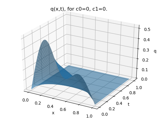
(a) Classical Dirichlet boundary conditions

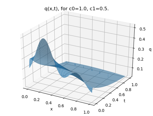
(b) Subcritical multipoint conditions

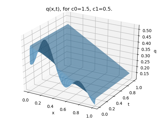
(c) Critical multipoint conditions

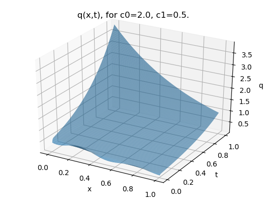
(d) Supercritical multipoint conditions

Figure 1: Solution of the 3-point problem (1.2) with initial datum a sum of two box functions, demonstrating the effects of sub/super/critical multipoint conditions on the qualitative behaviour of the solution

Remark 5.5.

The values such that $\frac{|c_{0}+c_{1}|}{2}=1$ correspond to the transition point between real and complex eigenvalues, but also yield the only case in which the eigenvalues are nonsimple. The multiplicity of the eigenvalues is the reason that the Green’s function approach of [3] fails for this case. However there is no impediment to using the approach we present.

Remark 5.6.

As suggested by the eigenvalues (5.26) and demonstrated by figures 1, the relaxation time of the system increases as the multipoint conditions approach criticality ($c_{0}+c_{1}\to 2^{-}$), but the steady state solution may be a little surprising for “Dirichlet-like” multipoint conditions. However, Neumann boundary values may be considered as appropriate limits of Dirichlet-like multipoint conditions which, in view of the below comparison, justifies the phenomenon.

By the usual arguments (see, for example, [29, §2.1.4]), the steady state solution must be a linear function $Q(x)=Ax+B$, and it is readily seen that the multipoint conditions imply

$$A=2B\left(\frac{c_{0}-1}{c_{0}}\right),\qquad A=2B\left(\frac{c_{1}-1}{2-c_{1}}\right).$$

If $c_{0}+c_{1}\neq 2$, it follows immediately that $A=B=0$, and the steady state solution is identically zero. However, if $c_{0}+c_{1}=2$ then this method is insufficient to yield the steady state solution.

This is a manifestation of the effect seen for the classical insulation (homogeneous Neumann) boundary conditions, arising in both cases from the presence of an eigenvalue at $0$. For the classical insulation case, after applying the boundary conditions, $A$ is known to be zero, but $B$ is free. The usual approach is to either

1. appeal to the physics of the problem: by the first law of thermodynamics, the constant steady state temperature must be the mean of the initial temperature profile, or

2. because $v(x,t)=q(x,t)-Q(x)\to 0$ as $t\to\infty$ and $v(x,0)=q_{0}(x)-Q(x)$, and all eigenfunctions but the first decay as $t\to\infty$, it must be that $q_{0}-Q$ is orthogonal to the first eigenfunction; this yields a new equation for the unknown constant function $Q$.

In our method, the contour deformation and residue calculation argument described in [32, 33, 19] may be used to find the contribution of the eigenfunction with eigenvalue at $0$, in terms of the Fourier transform of the initial datum. This approach is equivalent to (b). It is not known whether there is a method equivalent to (a) for this problem; it is not clear that the system should conserve energy.

In the supercritical case $c_{0}+c_{1}>2$, the existence of a negative eigenvalue causes the solution to blow up in the long time limit, rather than approach the $Q(x)=0$ steady state solution.

6 The case $n=3$: PDEs of third order

6.1 Dirichlet-to-Neumann map

In the case $n=3$, the linear system (4.12) may be expressed as

$$\Bigg{(}\overbrace{E_{r}(\lambda)\sum_{k=0}^{2}f_{k}^{r}(\lambda),E_{r}(\alpha\lambda)\sum_{k=0}^{2}\alpha^{2-k}f_{k}^{r}(\lambda),E_{r}(\alpha^{2}\lambda)\sum_{k=0}^{2}\alpha^{2(2-k)}f_{k}^{r}(\lambda)}^{r=0,1,\ldots,m}\Bigg{)}\mathcal{A}\\ =\Big{(}h_{0}(\lambda),h_{1}(\lambda),h_{2}(\lambda),\overbrace{-\hat{q}_{0}^{r}(\lambda),-\hat{q}_{0}^{r}(\alpha\lambda),-\hat{q}_{0}^{r}(\alpha^{2}\lambda)}^{r=1,2,\ldots,m}\Big{)}\\ +{\rm e}^{a\lambda^{n}\tau}\hat{q}_{\tau}^{r}\Big{(}0,0,0,\overbrace{\hat{q}_{\tau}^{r}(\lambda),\hat{q}_{\tau}^{r}(\alpha\lambda),\hat{q}_{\tau}^{r}(\alpha^{2}\lambda)}^{r=1,2,\ldots,m}\Big{)},$$ (6.1a)

where

$$\mathcal{A}=\setcounter{MaxMatrixCols}{13}\begin{pmatrix}B_{0\hskip 1.42262pt0}^{0}&B_{0\hskip 1.42262pt1}^{0}&B_{0\hskip 1.42262pt2}^{0}&-1&0&0&0&0&0&\cdots&0&0&0\\ B_{1\hskip 1.42262pt0}^{0}&B_{1\hskip 1.42262pt1}^{0}&B_{1\hskip 1.42262pt2}^{0}&0&-1&0&0&0&0&\cdots&0&0&0\\ B_{2\hskip 1.42262pt0}^{0}&B_{2\hskip 1.42262pt1}^{0}&B_{2\hskip 1.42262pt2}^{0}&0&0&-1&0&0&0&\cdots&0&0&0\\ B_{0\hskip 1.42262pt0}^{1}&B_{0\hskip 1.42262pt1}^{1}&B_{0\hskip 1.42262pt2}^{1}&1&0&0&-1&0&0&\cdots&0&0&0\\ B_{1\hskip 1.42262pt0}^{1}&B_{1\hskip 1.42262pt1}^{1}&B_{1\hskip 1.42262pt2}^{1}&0&1&0&0&-1&0&\cdots&0&0&0\\ B_{2\hskip 1.42262pt0}^{1}&B_{2\hskip 1.42262pt1}^{1}&B_{2\hskip 1.42262pt2}^{1}&0&0&1&0&0&-1&\cdots&0&0&0\\ B_{0\hskip 1.42262pt0}^{2}&B_{0\hskip 1.42262pt1}^{2}&B_{0\hskip 1.42262pt2}^{2}&0&0&0&1&0&0&\cdots&0&0&0\\ B_{1\hskip 1.42262pt0}^{2}&B_{1\hskip 1.42262pt1}^{2}&B_{1\hskip 1.42262pt2}^{2}&0&0&0&0&1&0&\cdots&0&0&0\\ B_{2\hskip 1.42262pt0}^{2}&B_{2\hskip 1.42262pt1}^{2}&B_{2\hskip 1.42262pt2}^{2}&0&0&0&0&0&1&\cdots&0&0&0\\ \vdots&\vdots&\vdots&\vdots&\vdots&\vdots&\vdots&\vdots&\vdots&\ddots&\vdots&\vdots&\vdots\\ B_{0\hskip 1.42262pt0}^{m}&B_{0\hskip 1.42262pt1}^{m}&B_{0\hskip 1.42262pt2}^{m}&0&0&0&0&0&0&\cdots&1&0&0\\ B_{1\hskip 1.42262pt0}^{m}&B_{1\hskip 1.42262pt1}^{m}&B_{1\hskip 1.42262pt2}^{m}&0&0&0&0&0&0&\cdots&0&1&0\\ B_{2\hskip 1.42262pt0}^{m}&B_{2\hskip 1.42262pt1}^{m}&B_{2\hskip 1.42262pt2}^{m}&0&0&0&0&0&0&\cdots&0&0&1\end{pmatrix},$$ (6.1b)

and, for $$k\in\{0,1,2\} r\in\{0,\ldots,m\}$$, ,

$$B_{0\hskip 1.42262ptk}^{r}(\lambda) =\frac{1}{3}E_{r}(-\lambda)\left[-\frac{b_{0\hskip 1.42262ptk}^{r}}{\lambda^{2}}+\frac{b_{1\hskip 1.42262ptk}^{r}}{i\lambda}+b_{2\hskip 1.42262ptk}^{r}\right],$$ (6.1c)

$$B_{1\hskip 1.42262ptk}^{r}(\lambda) =\frac{1}{3}E_{r}(-\alpha\lambda)\left[-\frac{\alpha b_{0\hskip 1.42262ptk}^{r}}{\lambda^{2}}+\frac{\alpha^{2}b_{1\hskip 1.42262ptk}^{r}}{i\lambda}+b_{2\hskip 1.42262ptk}^{r}\right]=B_{0\hskip 1.42262ptk}^{r}(\alpha\lambda),$$ (6.1d)

$$B_{2\hskip 1.42262ptk}^{r}(\lambda) =\frac{1}{3}E_{r}(-\alpha^{2}\lambda)\left[-\frac{\alpha^{2}b_{0\hskip 1.42262ptk}^{r}}{\lambda^{2}}+\frac{\alpha b_{1\hskip 1.42262ptk}^{r}}{i\lambda}+b_{2\hskip 1.42262ptk}^{r}\right]=B_{0\hskip 1.42262ptk}^{r}(\alpha^{2}\lambda).$$ (6.1e)

So $\mathcal{A}$ is the matrix with $1$ on the diagonal, $-1$ on the third super-diagonal, and $0$ elsewhere, with the first three columns replaced as shown.

In the following lemma, the index $s$ is understood to be an element of the group $\mathbb{Z}_{3}=\{0,1,2\}$ of integers modulo 3. The proof is presented in appendix A.

Lemma 6.1.

(a) The linear system

$$\Big{(}\overbrace{x_{0}^{r},x_{1}^{r},x_{2}^{r}}^{r=0,1,\ldots,m}\Big{)}\mathcal{A}=\Big{(}0,0,0,\overbrace{y_{0}^{r},y_{1}^{r},y_{2}^{r}}^{r=1,2,\ldots,m}\Big{)},$$ (6.2)

with $\mathcal{A}$ given by equation (6.1b) has solution

$$x_{s}^{r}=\frac{1}{\Delta(\lambda)}\Bigg{[}\sum_{j_{0},j_{1},j_{2}=0}^{m}\mathcal{D}(j_{0},j_{1},j_{2})L(j_{s},r,s)\\ +\frac{1}{2}\sum_{j_{0},j_{1},j_{2}=0}^{m}\mathcal{D}_{s\hskip 1.42262pts+1}(j_{0},j_{1},j_{2})L(j_{s},j_{s+1},s+1)\\ +\frac{1}{2}\sum_{j_{0},j_{1},j_{2}=0}^{m}\mathcal{D}_{s\hskip 1.42262pts+2}(j_{0},j_{1},j_{2})L(j_{s},j_{s+2},s+2)\Bigg{]},$$ (6.3)

where

$$\Delta(\lambda) =\sum_{j_{0},j_{1},j_{2}=0}^{m}\mathcal{D}(j_{0},j_{1},j_{2}),$$ (6.4)

$$L(j_{1},j_{2},s) =\left\{\begin{smallmatrix}1\text{{ if }}j_{1}<j_{2}\\ 0\text{{ if }}j_{1}=j_{2}\\ -1\text{{ if }}j_{1}>j_{2}\end{smallmatrix}\right\}\sum_{k=\min\{j_{1},j_{2}\}+1}^{\max\{j_{1},j_{2}\}}y_{s}^{k}(\lambda),$$ (6.5)

$$\mathcal{D}(j_{0},j_{1},j_{2}) =\det\begin{pmatrix}B_{0\hskip 1.42262pt0}^{j_{0}}&B_{0\hskip 1.42262pt1}^{j_{0}}&B_{0\hskip 1.42262pt2}^{j_{0}}\\ B_{1\hskip 1.42262pt0}^{j_{1}}&B_{1\hskip 1.42262pt1}^{j_{1}}&B_{1\hskip 1.42262pt2}^{j_{1}}\\ B_{2\hskip 1.42262pt0}^{j_{2}}&B_{2\hskip 1.42262pt1}^{j_{2}}&B_{2\hskip 1.42262pt2}^{j_{2}}\end{pmatrix},$$ (6.6)

and $\mathcal{D}_{s\hskip 1.42262ptp}(j_{0},j_{1},j_{2})$ is the matrix $\mathcal{D}(j_{0},j_{1},j_{2})$ with the row $(B_{s\hskip 1.42262pt0}^{j_{s}},B_{s\hskip 1.42262pt1}^{j_{s}},B_{s\hskip 1.42262pt2}^{j_{s}})$ replaced by $(B_{p\hskip 1.42262pt0}^{j_{s}},B_{p\hskip 1.42262pt1}^{j_{s}},B_{p\hskip 1.42262pt2}^{j_{s}})$.

(b) The linear system

$$\Big{(}\overbrace{x_{0}^{r},x_{1}^{r},x_{2}^{r}}^{r=0,1,\ldots,m}\Big{)}\mathcal{A}=\Big{(}h_{0},h_{1},h_{2},\overbrace{0,0,0}^{\mathchoice{\hbox to0.0pt{\hss$\displaystyle{r=1,2,\ldots,m}$\hss}}{\hbox to0.0pt{\hss$\textstyle{r=1,2,\ldots,m}$\hss}}{\hbox to0.0pt{\hss$\scriptstyle{r=1,2,\ldots,m}$\hss}}{\hbox to0.0pt{\hss$\scriptscriptstyle{r=1,2,\ldots,m}$\hss}}}\Big{)},$$ (6.7)

with $\mathcal{A}$ given by equation (6.1b) has solution

$$x_{s}^{r}(\lambda)=\frac{1}{\Delta(\lambda)}\sum_{j_{0},j_{1}=0}^{m}\left(h_{s}\mathcal{C}_{s+1\hskip 1.42262pts+2}^{s+1\hskip 1.42262pts+2}(j_{0},j_{1})+h_{s+1}\mathcal{C}_{s+2\hskip 1.42262pts}^{s+1\hskip 1.42262pts+2}(j_{0},j_{1})+h_{s+2}\mathcal{C}_{s\hskip 1.42262pts+1}^{s+1\hskip 1.42262pts+2}(j_{0},j_{1})\right),$$ (6.8)

where $\Delta(\lambda)$ is given by equation (6.4), and $\mathcal{C}$ are the boundary coefficient minors

$$\mathcal{C}_{p\hskip 1.42262ptq}^{u\hskip 1.42262ptv}(j_{0},j_{1})=\det\begin{pmatrix}B_{u\hskip 1.42262ptp}^{j_{0}}&B_{u\hskip 1.42262ptq}^{j_{0}}\\ B_{v\hskip 1.42262ptp}^{j_{1}}&B_{v\hskip 1.42262ptq}^{j_{1}}\end{pmatrix}.$$ (6.9)

Rather than deriving general conditions analogous to the ones found in section 5.2, that guarantee that the terms involving the unknown function $\hat{q}^{r}_{\tau}(\lambda)$, we will now compute an explicit example.

6.2 An explicit example: a 3-point case for $n=3$

Consider the initial-multipoint value problem for the PDE $q_{t}+q_{xxx}=0$ ($n=3$, $a=-i$) obtained by setting $m=2$, $\eta_{1}=\frac{1}{2}$ and prescribing the three multipoint conditions

$$q(0,t)-cq(\tfrac{1}{2},t)=0,\qquad q(1,t)=0,\qquad q_{x}(1,t)=0.$$ (6.10)

This example is not motivated by any application of which we are aware, but it is a natural third order analogue of the example considered in section 5.3. In addition, these particular conditions are the simplest generalization of the boundary conditions $q(0,t)=q(1,t)=q_{x}(1,t)=0$, which are known to destroy the self-adjoint structure of the spatial operator. Hence they are interesting from the purely mathematical point of view, and for this reason we include this as our example.

The given conditions correspond to the choice

$$\begin{pmatrix}b_{0\hskip 1.42262pt0}^{0}&b_{0\hskip 1.42262pt1}^{0}&b_{0\hskip 1.42262pt2}^{0}\\ b_{1\hskip 1.42262pt0}^{0}&b_{1\hskip 1.42262pt1}^{0}&b_{1\hskip 1.42262pt2}^{0}\\ b_{2\hskip 1.42262pt0}^{0}&b_{2\hskip 1.42262pt1}^{0}&b_{2\hskip 1.42262pt2}^{0}\\ b_{0\hskip 1.42262pt0}^{1}&b_{0\hskip 1.42262pt1}^{1}&b_{0\hskip 1.42262pt2}^{1}\\ b_{1\hskip 1.42262pt0}^{1}&b_{1\hskip 1.42262pt1}^{1}&b_{1\hskip 1.42262pt2}^{1}\\ b_{2\hskip 1.42262pt0}^{1}&b_{2\hskip 1.42262pt1}^{1}&b_{2\hskip 1.42262pt2}^{1}\\ b_{0\hskip 1.42262pt0}^{2}&b_{0\hskip 1.42262pt1}^{2}&b_{0\hskip 1.42262pt2}^{2}\\ b_{1\hskip 1.42262pt0}^{2}&b_{1\hskip 1.42262pt1}^{2}&b_{1\hskip 1.42262pt2}^{2}\\ b_{2\hskip 1.42262pt0}^{2}&b_{2\hskip 1.42262pt1}^{2}&b_{2\hskip 1.42262pt2}^{2}\end{pmatrix}=\begin{pmatrix}1&0&0\\ 0&0&0\\ 0&0&0\\ -c&0&0\\ 0&0&0\\ 0&0&0\\ 0&1&0\\ 0&0&1\\ 0&0&0\end{pmatrix},\qquad\begin{pmatrix}B_{0\hskip 1.42262pt0}^{0}&B_{0\hskip 1.42262pt1}^{0}&B_{0\hskip 1.42262pt2}^{0}\\ B_{1\hskip 1.42262pt0}^{0}&B_{1\hskip 1.42262pt1}^{0}&B_{1\hskip 1.42262pt2}^{0}\\ B_{2\hskip 1.42262pt0}^{0}&B_{2\hskip 1.42262pt1}^{0}&B_{2\hskip 1.42262pt2}^{0}\\ B_{0\hskip 1.42262pt0}^{1}&B_{0\hskip 1.42262pt1}^{1}&B_{0\hskip 1.42262pt2}^{1}\\ B_{1\hskip 1.42262pt0}^{1}&B_{1\hskip 1.42262pt1}^{1}&B_{1\hskip 1.42262pt2}^{1}\\ B_{2\hskip 1.42262pt0}^{1}&B_{2\hskip 1.42262pt1}^{1}&B_{2\hskip 1.42262pt2}^{1}\\ B_{0\hskip 1.42262pt0}^{2}&B_{0\hskip 1.42262pt1}^{2}&B_{0\hskip 1.42262pt2}^{2}\\ B_{1\hskip 1.42262pt0}^{2}&B_{1\hskip 1.42262pt1}^{2}&B_{1\hskip 1.42262pt2}^{2}\\ B_{2\hskip 1.42262pt0}^{2}&B_{2\hskip 1.42262pt1}^{2}&B_{2\hskip 1.42262pt2}^{2}\end{pmatrix}=\begin{pmatrix}\frac{-1}{3\lambda^{2}}&0&0\\ \frac{-\alpha}{3\lambda^{2}}&0&0\\ \frac{-\alpha^{2}}{3\lambda^{2}}&0&0\\ \frac{c}{3\lambda^{2}}{\rm e}^{i\lambda/2}&0&0\\ \frac{\alpha c}{3\lambda^{2}}{\rm e}^{i\alpha\lambda/2}&0&0\\ \frac{\alpha^{2}c}{3\lambda^{2}}{\rm e}^{i\alpha^{2}\lambda/2}&0&0\\ 0&\frac{-1}{3\lambda^{2}}{\rm e}^{i\lambda}&\frac{1}{3i\lambda}{\rm e}^{i\lambda}\\ 0&\frac{-\alpha}{3\lambda^{2}}{\rm e}^{i\alpha\lambda}&\frac{\alpha^{2}}{3i\lambda}{\rm e}^{i\alpha\lambda}\\ 0&\frac{-\alpha^{2}}{3\lambda^{2}}{\rm e}^{i\alpha^{2}\lambda}&\frac{\alpha}{3i\lambda}{\rm e}^{i\alpha^{2}\lambda}\end{pmatrix}.$$

It follows that

$$\Delta(\lambda)=\frac{\alpha^{2}-\alpha}{27i\lambda^{5}}\sum_{k=0}^{2}\alpha^{k}\left({\rm e}^{-i\alpha^{k}\lambda}-c{\rm e}^{-i\alpha^{k}\lambda/2}\right),$$

and, applying lemma 6.1(a) with $y_{s}^{r}(\lambda)=\hat{q}_{\tau}^{r}(\alpha^{s}\lambda)$,

$$x_{0}^{0}(\lambda) =\frac{\alpha^{2}-\alpha}{27i\lambda^{5}\Delta(\lambda)}\Bigg{[}-c{\rm e}^{-i\lambda/2}\hat{q}_{\tau}^{1}(\lambda)$$

$$\phantom{=a{}}-\left\{\alpha\left({\rm e}^{-i\alpha\lambda}-c{\rm e}^{-i\alpha\lambda/2}\right)+\alpha^{2}\left({\rm e}^{-i\alpha^{2}\lambda}-c{\rm e}^{-i\alpha^{2}\lambda/2}\right)\right\}\left(\hat{q}_{\tau}^{1}(\lambda)+\hat{q}_{\tau}^{2}(\lambda)\right)$$

$$\phantom{=a{}}+{\rm e}^{-i\lambda}\left\{\alpha\left(\hat{q}_{\tau}^{1}(\alpha\lambda)+\left(1-c{\rm e}^{i\alpha\lambda/2}\right)\hat{q}_{\tau}^{2}(\alpha\lambda)\right)+\alpha^{2}\left(\hat{q}_{\tau}^{1}(\alpha^{2}\lambda)+\left(1-c{\rm e}^{i\alpha^{2}\lambda/2}\right)\hat{q}_{\tau}^{2}(\alpha^{2}\lambda)\right)\right\}\Bigg{]},$$

$$x_{0}^{2}(\lambda) =\frac{\alpha^{2}-\alpha}{27i\lambda^{5}\Delta(\lambda)}{\rm e}^{-i\lambda}\sum_{k=0}^{2}\alpha^{k}\left(\hat{q}_{\tau}^{1}(\alpha^{k}\lambda)+\left(1-c{\rm e}^{i\alpha^{k}\lambda/2}\right)\hat{q}_{\tau}^{2}(\alpha^{k}\lambda)\right).$$

From here, a simple asymptotic analysis yields

$$x_{0}^{0}(\lambda) =\mathcal{O}(\lambda^{-1}) \mbox{ as }\lambda \to\infty\mbox{ from within } \overline{D_{R}^{+}},$$

$$x_{0}^{2}(\lambda) =\mathcal{O}({\rm e}^{-i\lambda}\lambda^{-1}) \mbox{ as }\lambda \to\infty\mbox{ from within } \overline{D_{R}^{-}}.$$

This asymptotic result plays the role of lemma 5.2, which enables a Jordan’s lemma argument of the type found in the proof of proposition 5.3. In this case, the theory of zeros of exponential sums [20] immediately yields that, for $R>0$ sufficiently large, $\Delta$ has no zeros in $\overline{D_{R}}$. Thus the terms involving $\hat{q}_{\tau}^{r}$ make no contribution to the solution representation.

Remark 6.2.

We stress that the above result holds if and only if $a=-i$; if and only if the partial differential equation is

$$q_{t}+q_{xxx}=0.$$

Choosing $a=i$ with the same multipoint conditions specifies an ill-posed problem. This is in accordance with the results of [26], in which the above example is studied for $c=0$, and it is shown that the problem is well-posed for $a=-i$ only.

7 Conclusions

We have derived explicit formulae for the solution of a large class of nonlocal boundary value problems, by formulating them as multipoint value problems and generalising the machinery of the Fokas transform to multipoint value problems. While we have derived the set-up for linear PDEs of arbitrary order, the formulae have been derived explicitly for PDEs of order $n=2$ and $n=3$.

Even though the general expression is quite cumbersome, the derivation is algorithmic, and the final result fully explicit. In specific examples, it is possible to simply apply these formulae to find a general expression for the solution. This expression is always in the form of a uniformly convergent integral that can be evaluated numerically in a very efficient manner by numerical complex integration, taking advantage of the analyticity properties of the solution to select an integration contour of fast decay, as done in [10, 19].

We have studied also some specific examples of second and third order problems, and given criteria that guarantee that the solution representation depends effectively only on the given data of the problem, at least for $n=2$. The full characterisation of multipoint conditions that yield well posed problems, and the analysis of the cases when the integral representation is equivalent to a series representation, are left for a future publication.

Appendix A Appendix: Proof of Lemma 5.1 and Lemma 6.1

A.1 Linear system for $n=2$

Proof of lemma 5.1(a).

A constructive proof may be obtained via Cramer’s rule, Laplace’s formula and lemma A.1. However the argument is somewhat complex. Instead, we present a direct verification of the validity of the solution. It must be shown that, for each $r\in\{1,\ldots,m\}$,

$$x_{r}-x_{r-1} =y_{r},$$ (A.1)

$$X_{r}-X_{r-1} =Y_{r},$$ (A.2)

and that, for each $s\in\{0,1\}$,

$$\Delta(\lambda)\sum_{r=0}^{m}\left(B_{0\hskip 1.42262pts}^{r}x_{r}(\lambda)+B_{1\hskip 1.42262pts}^{r}X_{r}(\lambda)\right)=0,$$ (A.3)

with $x_{r}$, $X_{r}$ defined by equations (5.3) and (5.4).

Fixing $r\in\{1,\ldots,m\}$, it is immediate that

$$x_{r}-x_{r-1}=\frac{1}{\Delta(\lambda)}\sum_{j,k=0}^{m}\left[B_{0\hskip 1.42262pt0}^{j}B_{1\hskip 1.42262pt1}^{k}-B_{1\hskip 1.42262pt0}^{k}B_{0\hskip 1.42262pt1}^{j}\right]\\ \Bigg{(}\left\{\begin{smallmatrix}1\text{{ if }}j<r\\ 0\text{{ if }}j=r\\ -1\text{{ if }}j>r\end{smallmatrix}\right\}\sum_{l=\min\{j,r\}+1}^{\max\{j,r\}}y_{l}(\lambda)-\left\{\begin{smallmatrix}1\text{{ if }}j<r-1\\ 0\text{{ if }}j=r-1\\ -1\text{{ if }}j>r-1\end{smallmatrix}\right\}\sum_{l=\min\{j,r-1\}+1}^{\max\{j,r-1\}}y_{l}(\lambda)\Bigg{)}.$$ (A.4)

Note that the latter term in expression (5.3) is independent of $r$, so the corresponding terms from $x_{r-1}$ and $x_{r}$ cancel. A case-by-case ($j<r-1$, $j=r-1$, $j=r$, $j>r$) evaluation yields that the parenthetical quantity in equation (A.4) evaluates to $y_{r}(\lambda)$ for all $j$. A substitution of representation (5.5) for $\Delta(\lambda)$, and cancellation, completes the proof of equation (A.1). The proof of equation (A.2) is very similar.

With $s=0$, the left hand side of equation (A.3) expands to

$$\sum_{r,j,k=0}^{m}B_{0\hskip 1.42262pt0}^{r}\left[B_{0\hskip 1.42262pt0}^{j}B_{1\hskip 1.42262pt1}^{k}-B_{1\hskip 1.42262pt0}^{k}B_{0\hskip 1.42262pt1}^{j}\right]\left\{\begin{smallmatrix}1\text{{ if }}j<r\\ 0\text{{ if }}j=r\\ -1\text{{ if }}j>r\end{smallmatrix}\right\}\sum_{l=\min\{j,r\}+1}^{\max\{j,r\}}y_{l}(\lambda)\\ -\frac{1}{2}\sum_{r,j,k=0}^{m}B_{1\hskip 1.42262pt0}^{r}\left[B_{0\hskip 1.42262pt0}^{j}B_{0\hskip 1.42262pt1}^{k}-B_{0\hskip 1.42262pt0}^{k}B_{0\hskip 1.42262pt1}^{j}\right]\left\{\begin{smallmatrix}1\text{{ if }}j<k\\ 0\text{{ if }}j=k\\ -1\text{{ if }}j>k\end{smallmatrix}\right\}\sum_{l=\min\{j,k\}+1}^{\max\{j,k\}}y_{l}(\lambda)\\ +\sum_{r,j,k=0}^{m}B_{1\hskip 1.42262pt0}^{r}\left[B_{0\hskip 1.42262pt0}^{j}B_{1\hskip 1.42262pt1}^{k}-B_{1\hskip 1.42262pt0}^{k}B_{0\hskip 1.42262pt1}^{j}\right]\left\{\begin{smallmatrix}1\text{{ if }}k<r\vphantom{j}\\ 0\text{{ if }}k=r\vphantom{j}\\ -1\text{{ if }}k>r\vphantom{j}\end{smallmatrix}\right\}\sum_{l=\min\{k,r\}+1}^{\max\{k,r\}}Y_{l}(\lambda)\\ +\frac{1}{2}\sum_{r,j,k=0}^{m}B_{0\hskip 1.42262pt0}^{r}\left[B_{1\hskip 1.42262pt0}^{j}B_{1\hskip 1.42262pt1}^{k}-B_{1\hskip 1.42262pt0}^{k}B_{1\hskip 1.42262pt1}^{j}\right]\left\{\begin{smallmatrix}1\text{{ if }}j<k\\ 0\text{{ if }}j=k\\ -1\text{{ if }}j>k\end{smallmatrix}\right\}\sum_{l=\min\{j,k\}+1}^{\max\{j,k\}}Y_{l}(\lambda).$$ (A.5)

Informed by the fact that $y_{l}$, $Y_{l}$ are linearly independent, we aim to show that the third and fourth terms of expression (A.5) cancel. Adding and subtracting $B_{1\hskip 1.42262pt0}^{j}B_{1\hskip 1.42262pt0}^{k}B_{0\hskip 1.42262pt1}^{r}$, it holds that

$$B_{0\hskip 1.42262pt0}^{r}\left[B_{1\hskip 1.42262pt0}^{j}B_{1\hskip 1.42262pt1}^{k}-B_{1\hskip 1.42262pt0}^{k}B_{1\hskip 1.42262pt1}^{j}\right]=B_{1\hskip 1.42262pt0}^{j}\left[B_{0\hskip 1.42262pt0}^{r}B_{1\hskip 1.42262pt1}^{k}-B_{1\hskip 1.42262pt0}^{k}B_{0\hskip 1.42262pt1}^{r}\right]-B_{1\hskip 1.42262pt0}^{k}\left[B_{0\hskip 1.42262pt0}^{r}B_{1\hskip 1.42262pt1}^{j}-B_{1\hskip 1.42262pt0}^{j}B_{0\hskip 1.42262pt1}^{r}\right].$$ (A.6)

Hence the fourth term of expression (A.5) is equal to

$$\frac{1}{2}\Bigg{(}\sum_{r,j,k=0}^{m}B_{1\hskip 1.42262pt0}^{j}\left[B_{0\hskip 1.42262pt0}^{r}B_{1\hskip 1.42262pt1}^{k}-B_{1\hskip 1.42262pt0}^{k}B_{0\hskip 1.42262pt1}^{r}\right]\left\{\begin{smallmatrix}1\text{{ if }}j<k\\ 0\text{{ if }}j=k\\ -1\text{{ if }}j>k\end{smallmatrix}\right\}\sum_{l=\min\{j,k\}+1}^{\max\{j,k\}}Y_{l}(\lambda)\\ -\sum_{r,j,k=0}^{m}B_{1\hskip 1.42262pt0}^{k}\left[B_{0\hskip 1.42262pt0}^{r}B_{1\hskip 1.42262pt1}^{j}-B_{1\hskip 1.42262pt0}^{j}B_{0\hskip 1.42262pt1}^{r}\right]\left\{\begin{smallmatrix}1\text{{ if }}j<k\\ 0\text{{ if }}j=k\\ -1\text{{ if }}j>k\end{smallmatrix}\right\}\sum_{l=\min\{j,k\}+1}^{\max\{j,k\}}Y_{l}(\lambda)\Bigg{)}.$$ (A.7)

Applying the permutation $(j,r,k)\mapsto(r,j,k)$ to the indices in the first sum of expression (A.7), and the permutation $(k,r,j)\mapsto(r,j,k)$ to the indices in the second sum of expression (A.7), we obtain

$$\frac{1}{2}\Bigg{(}\sum_{r,j,k=0}^{m}B_{1\hskip 1.42262pt0}^{r}\left[B_{0\hskip 1.42262pt0}^{j}B_{1\hskip 1.42262pt1}^{k}-B_{1\hskip 1.42262pt0}^{k}B_{0\hskip 1.42262pt1}^{j}\right]\left\{\begin{smallmatrix}1\text{{ if }}r<k\vphantom{j}\\ 0\text{{ if }}r=k\vphantom{j}\\ -1\text{{ if }}r>k\vphantom{j}\end{smallmatrix}\right\}\sum_{l=\min\{r,k\}+1}^{\max\{r,k\}}Y_{l}(\lambda)\\ -\sum_{r,j,k=0}^{m}B_{1\hskip 1.42262pt0}^{r}\left[B_{0\hskip 1.42262pt0}^{j}B_{1\hskip 1.42262pt1}^{k}-B_{1\hskip 1.42262pt0}^{k}B_{0\hskip 1.42262pt1}^{j}\right]\left\{\begin{smallmatrix}1\text{{ if }}k<r\vphantom{j}\\ 0\text{{ if }}k=r\vphantom{j}\\ -1\text{{ if }}k>r\vphantom{j}\end{smallmatrix}\right\}\sum_{l=\min\{k,r\}+1}^{\max\{k,r\}}Y_{l}(\lambda)\Bigg{)},$$ (A.8)

which, by

$$\left\{\begin{smallmatrix}1\text{{ if }}r<k\vphantom{j}\\ 0\text{{ if }}r=k\vphantom{j}\\ -1\text{{ if }}r>k\vphantom{j}\end{smallmatrix}\right\}=-\left\{\begin{smallmatrix}1\text{{ if }}k<r\vphantom{j}\\ 0\text{{ if }}k=r\vphantom{j}\\ -1\text{{ if }}k>r\vphantom{j}\end{smallmatrix}\right\},$$

is equal to

$$-\sum_{r,j,k=0}^{m}B_{1\hskip 1.42262pt0}^{r}\left[B_{0\hskip 1.42262pt0}^{j}B_{1\hskip 1.42262pt1}^{k}-B_{1\hskip 1.42262pt0}^{k}B_{0\hskip 1.42262pt1}^{j}\right]\left\{\begin{smallmatrix}1\text{{ if }}k<r\vphantom{j}\\ 0\text{{ if }}k=r\vphantom{j}\\ -1\text{{ if }}k>r\vphantom{j}\end{smallmatrix}\right\}\sum_{l=\min\{k,r\}+1}^{\max\{k,r\}}Y_{l}(\lambda).$$

Hence the third and fourth terms of expression (A.5) cancel. Similarly, the first and second terms in (A.5) cancel. This completes the proof of equation (A.3) for $s=0$. A similar argument yields equation (A.3) for $s=1$. ∎

Proof of lemma 5.1(b).

The definitions (5.7), (5.8) of $x_{r}$ and $X_{r}$ are independent of $r$, so they must satisfy $x_{r}-x_{r-1}=0=X_{r}-X_{r-1}$. A simple evaluation establishes that

$$\sum_{r=0}^{m}\left(B_{0\hskip 1.42262pt0}^{r}x_{r}+B_{1\hskip 1.42262pt0}^{r}X_{r}\right)=h_{0},\qquad\sum_{r=0}^{m}\left(B_{0\hskip 1.42262pt1}^{r}x_{r}+B_{1\hskip 1.42262pt1}^{r}X_{r}\right)=h_{1}.\qed$$

A.2 Linear system for $n=3$

Proof of lemma 6.1(a).

We begin by noting some useful identities. Evaluating the definition (6.5) of $L$, at each of $j_{s}<r-1$, $j_{s}=r-1$, $j_{s}=r$, and $j_{s}>r$,

$$L(j_{s},r,s)-L(j_{s},r-1,s)=y_{s}^{r}.$$ (A.9)

It is also immediately apparent from the definition that

$$L(j_{1},j_{2},s)=-L(j_{2},j_{1},s).$$ (A.10)

By a row swap, the boundary coefficient minors have the property

$$\mathcal{C}_{p\hskip 1.42262ptq}^{u\hskip 1.42262ptv}(j_{0},j_{1})=-\mathcal{C}_{p\hskip 1.42262ptq}^{v\hskip 1.42262ptu}(j_{1},j_{0}).$$ (A.11)

Expanding in minors, for any $s,p\in\mathbb{Z}_{3}$,

$$\mathcal{D}(j_{0},j_{1},j_{2}) =B_{s\hskip 1.42262ptp}^{j_{s}}\mathcal{C}_{p+1\hskip 1.42262ptp+2}^{s+1\hskip 1.42262pts+2}(j_{s+1},j_{s+2})+B_{s+1\hskip 1.42262ptp}^{j_{s+1}}\mathcal{C}_{p+1\hskip 1.42262ptp+2}^{s+2\hskip 1.42262pts}(j_{s+2},j_{s})+B_{s+2\hskip 1.42262ptp}^{j_{s+2}}\mathcal{C}_{p+1\hskip 1.42262ptp+2}^{s\hskip 1.42262pts+1}(j_{s},j_{s+1}),$$ (A.12a)

$$\mathcal{D}_{s\hskip 1.42262pts+1}(j_{0},j_{1},j_{2}) =B_{s\hskip 1.42262ptp}^{j_{s}}\mathcal{C}_{p+1\hskip 1.42262ptp+2}^{s\hskip 1.42262pts+2}(j_{s+1},j_{s+2})+B_{s\hskip 1.42262ptp}^{j_{s+1}}\mathcal{C}_{p+1\hskip 1.42262ptp+2}^{s+2\hskip 1.42262pts}(j_{s+2},j_{s})+B_{s+2\hskip 1.42262ptp}^{j_{s+2}}\mathcal{C}_{p+1\hskip 1.42262ptp+2}^{s\hskip 1.42262pts}(j_{s},j_{s+1}),$$ (A.12b)

$$\mathcal{D}_{s\hskip 1.42262pts+2}(j_{0},j_{1},j_{2}) =B_{s\hskip 1.42262ptp}^{j_{s}}\mathcal{C}_{p+1\hskip 1.42262ptp+2}^{s+1\hskip 1.42262pts}(j_{s+1},j_{s+2})+B_{s+1\hskip 1.42262ptp}^{j_{s+1}}\mathcal{C}_{p+1\hskip 1.42262ptp+2}^{s\hskip 1.42262pts}(j_{s+2},j_{s})+B_{s\hskip 1.42262ptp}^{j_{s+2}}\mathcal{C}_{p+1\hskip 1.42262ptp+2}^{s\hskip 1.42262pts+1}(j_{s},j_{s+1}).$$ (A.12c)

We must establish both

$$x_{s}^{r}-x_{s}^{r-1}=y_{s}^{r}\qquad\hskip 2.84526pt\forall\hskip 2.84526ptr\in\{1,2,\ldots,m\},\;s\in\mathbb{Z}_{3},$$ (A.13)

and

$$2\Delta(\lambda)\sum_{r=0}^{m}\sum_{s=0}^{2}B_{s\hskip 1.42262ptp}^{r}x_{s}^{r}=0\qquad\hskip 2.84526pt\forall\hskip 2.84526ptp\in\mathbb{Z}_{3}.$$ (A.14)

Note that, in the definition (6.3) of $x_{s}^{r}$, the second and third triple-sums are independent of $r$. Therefore they cancel in the difference $x_{s}^{r}-x_{s}^{r-1}$. Hence

$$x_{s}^{r}-x_{s}^{r-1}=\frac{1}{\Delta(\lambda)}\sum_{j_{0},j_{1},j_{2}=0}^{m}\mathcal{D}(j_{0},j_{1},j_{2})[L(j_{s},r,s)-L(j_{s},r-1,s)]=\frac{1}{\Delta(\lambda)}\Delta(\lambda)y_{s}^{r},$$

by equation (A.9). Hence (A.13) holds.

Substituting the definition of $x_{s}^{r}$, expanding the sum over $s$, collating terms with like numbers in the final argument of $L$, and re-expressing as a sum over $s$, the left hand side of equation (A.14) may be expressed as

$$\sum_{s=0}^{2}\Bigg{[}2\sum_{r,j_{0},j_{1},j_{2}=0}^{m}B_{s\hskip 1.42262ptp}^{r}\mathcal{D}(j_{0},j_{1},j_{2})L(j_{s},r,s)\\ +\sum_{r,j_{0},j_{1},j_{2}=0}^{m}B_{s+2\hskip 1.42262ptp}^{r}\mathcal{D}_{s\hskip 1.42262pts+2}(j_{0},j_{1},j_{2})L(j_{s+2},j_{s},s)\\ +\sum_{r,j_{0},j_{1},j_{2}=0}^{m}B_{s+1\hskip 1.42262ptp}^{r}\mathcal{D}_{s\hskip 1.42262pts+1}(j_{0},j_{1},j_{2})L(j_{s+1},j_{s},s)\Bigg{]}$$

Using equations (A.12) to expand the determinants $\mathcal{D}$ in their minors, the bracket evaluates to

$$2\sum_{r,j_{0},j_{1},j_{2}=0}^{m}B_{s\hskip 1.42262ptp}^{r}B_{s\hskip 1.42262ptp}^{j_{s}}\mathcal{C}_{p+1\hskip 1.42262ptp+2}^{s+1\hskip 1.42262pts+2}(j_{s+1},j_{s+2})L(j_{s},r,s)\\ +2\sum_{r,j_{0},j_{1},j_{2}=0}^{m}B_{s\hskip 1.42262ptp}^{r}B_{s+1\hskip 1.42262ptp}^{j_{s+1}}\mathcal{C}_{p+1\hskip 1.42262ptp+2}^{s+2\hskip 1.42262pts}(j_{s+2},j_{s})L(j_{s},r,s)\\ +2\sum_{r,j_{0},j_{1},j_{2}=0}^{m}B_{s\hskip 1.42262ptp}^{r}B_{s+2\hskip 1.42262ptp}^{j_{s+2}}\mathcal{C}_{p+1\hskip 1.42262ptp+2}^{s\hskip 1.42262pts+1}(j_{s},j_{s+1})L(j_{s},r,s)\\ +\sum_{r,j_{0},j_{1},j_{2}=0}^{m}B_{s+2\hskip 1.42262ptp}^{r}B_{s\hskip 1.42262ptp}^{j_{s}}\mathcal{C}_{p+1\hskip 1.42262ptp+2}^{s+1\hskip 1.42262pts}(j_{s+1},j_{s+2})L(j_{s+2},j_{s},s)\\ +\sum_{r,j_{0},j_{1},j_{2}=0}^{m}B_{s+2\hskip 1.42262ptp}^{r}B_{s+1\hskip 1.42262ptp}^{j_{s+1}}\mathcal{C}_{p+1\hskip 1.42262ptp+2}^{s\hskip 1.42262pts}(j_{s+2},j_{s})L(j_{s+2},j_{s},s)\\ +\sum_{r,j_{0},j_{1},j_{2}=0}^{m}B_{s+2\hskip 1.42262ptp}^{r}B_{s\hskip 1.42262ptp}^{j_{s+2}}\mathcal{C}_{p+1\hskip 1.42262ptp+2}^{s\hskip 1.42262pts+1}(j_{s},j_{s+1})L(j_{s+2},j_{s},s)\\ +\sum_{r,j_{0},j_{1},j_{2}=0}^{m}B_{s+1\hskip 1.42262ptp}^{r}B_{s\hskip 1.42262ptp}^{j_{s}}\mathcal{C}_{p+1\hskip 1.42262ptp+2}^{s\hskip 1.42262pts+2}(j_{s+1},j_{s+2})L(j_{s+1},j_{s},s)\\ +\sum_{r,j_{0},j_{1},j_{2}=0}^{m}B_{s+1\hskip 1.42262ptp}^{r}B_{s\hskip 1.42262ptp}^{j_{s+1}}\mathcal{C}_{p+1\hskip 1.42262ptp+2}^{s+2\hskip 1.42262pts}(j_{s+2},j_{s})L(j_{s+1},j_{s},s)\\ +\sum_{r,j_{0},j_{1},j_{2}=0}^{m}B_{s+1\hskip 1.42262ptp}^{r}B_{s+2\hskip 1.42262ptp}^{j_{s+2}}\mathcal{C}_{p+1\hskip 1.42262ptp+2}^{s\hskip 1.42262pts}(j_{s},j_{s+1})L(j_{s+1},j_{s},s)$$ (A.15)

In the first line of expression (A.15) there are two identical quadruple-sums. We switch the roles of indices $r\leftrightarrow j_{s}$ in one of these sums and see that the summand evaluates to

$$\mbox{(summand of other sum in line 1)}\frac{L(r,j_{s},s)}{L(j_{s},r,s)}.$$

Hence, by equation (A.10), the two quadruple-sums in the first line cancel.

In line 5, we apply the map $(r,j_{s},j_{s+1},j_{s+2})\mapsto(j_{s+2},j_{s+1},r,j_{s})$, and equation (A.10) to see that the sum on line 5 cancels with the sum on line 9.

In line 4, we apply the map $(r,j_{s},j_{s+1},j_{s+2})\mapsto(j_{s+2},r,j_{s+1},j_{s})$, and equation (A.11). In line 6, we apply the map $(r,j_{s},j_{s+1},j_{s+2})\mapsto(j_{s+2},j_{s},j_{s+1},r)$, and equation (A.10). Hence line 3 cancels with lines 4 and 6.

In line 7, we apply the map $(r,j_{s},j_{s+1},j_{s+2})\mapsto(j_{s+1},r,j_{s},j_{s+2})$, and equation (A.11). In line 8, we apply the map $(r,j_{s},j_{s+1},j_{s+2})\mapsto(j_{s+1},j_{s},r,j_{s+2})$, and equation (A.10). Hence line 2 cancels with lines 7 and 8.

We have established that expression (A.15) evaluates to $0$, so (A.14) holds. ∎

Proof of lemma 6.1(b).

By definition (6.8), $x_{s}^{r}$ is independent of $r$, so $x_{s}^{r}-x_{s}^{r-1}=0$. For each $p\in\mathbb{Z}_{3}$, we expand

$$\sum_{r=0}^{m}\sum_{s=0}^{2}B_{s\hskip 1.42262ptp}^{r}x_{s}^{r}=\\ \frac{1}{\Delta}\sum_{r,j_{0},j_{1}=0}^{m}\Bigg{[}\sum_{s=0}^{2}B_{s\hskip 1.42262ptp}^{r}h_{s}\mathcal{C}_{s+1\hskip 1.42262pts+2}^{s+1\hskip 1.42262pts+2}(j_{0},j_{1})+\sum_{s=0}^{2}B_{s\hskip 1.42262ptp}^{r}h_{s+1}\mathcal{C}_{s+2\hskip 1.42262pts}^{s+1\hskip 1.42262pts+2}(j_{0},j_{1})+\sum_{s=0}^{2}B_{s\hskip 1.42262ptp}^{r}h_{s+2}\mathcal{C}_{s\hskip 1.42262pts+1}^{s+1\hskip 1.42262pts+2}(j_{0},j_{1})\Bigg{]}.$$

As $\{s,s+1,s+2\}=\{0,1,2\}=\{p,p+1,p+2\}$ are all representations of $\mathbb{Z}_{3}$, we reindex the sums over $s$ as $\sum_{s=p}^{p+2}$ on the right hand side. Then the bracket evaluates to

$$h_{p}\Big{(}B_{p\hskip 1.42262ptp}^{r}\mathcal{C}_{p+1\hskip 1.42262ptp+2}^{p+1\hskip 1.42262ptp+2}(j_{0},j_{1})+B_{p+1\hskip 1.42262ptp}^{r}\mathcal{C}_{p+1\hskip 1.42262ptp+2}^{p+2\hskip 1.42262ptp}(j_{0},j_{1})+B_{p+2\hskip 1.42262ptp}^{r}\mathcal{C}_{p+1\hskip 1.42262ptp+2}^{p\hskip 1.42262ptp+1}(j_{0},j_{1})\Big{)}\\ +h_{p+1}\Big{(}B_{p+1\hskip 1.42262ptp}^{r}\mathcal{C}_{p+2\hskip 1.42262ptp}^{p+2\hskip 1.42262ptp}(j_{0},j_{1})+B_{p+2\hskip 1.42262ptp}^{r}\mathcal{C}_{p+2\hskip 1.42262ptp}^{p\hskip 1.42262ptp+1}(j_{0},j_{1})+B_{p\hskip 1.42262ptp}^{r}\mathcal{C}_{p+2\hskip 1.42262ptp}^{p+1\hskip 1.42262ptp+2}(j_{0},j_{1})\Big{)}\\ +h_{p+2}\Big{(}B_{p+2\hskip 1.42262ptp}^{r}\mathcal{C}_{p\hskip 1.42262ptp+1}^{p\hskip 1.42262ptp+1}(j_{0},j_{1})+B_{p\hskip 1.42262ptp}^{r}\mathcal{C}_{p\hskip 1.42262ptp+1}^{p+1\hskip 1.42262ptp+2}(j_{0},j_{1})+B_{p+1\hskip 1.42262ptp}^{r}\mathcal{C}_{p\hskip 1.42262ptp+1}^{p+2\hskip 1.42262ptp}(j_{0},j_{1})\Big{)}.$$ (A.16)

As each term in expression (A.16) is summed over $r,j_{0},j_{1}$ separately, we can cyclically permute the indices $(r,j_{0},j_{1})\mapsto(j_{0},j_{1},r)$ in the second term on each line of (A.16), and $(r,j_{0},j_{1})\mapsto(j_{1},r,j_{0})$ in the third term on each line of (A.16). It is then immediate from the definition of $\mathcal{C}$, that the first line of (A.16) evalutes to $h_{p}\mathcal{D}(r,j_{0},j_{1})$. However, the second and third lines of (A.16) evaluate to

$$h_{p+1}\det\begin{pmatrix}B_{p+1\hskip 1.42262ptp}^{r}&B_{p+1\hskip 1.42262ptp+2}^{r}&B_{p+1\hskip 1.42262ptp}^{r}\\ B_{p+2\hskip 1.42262ptp}^{j_{0}}&B_{p+2\hskip 1.42262ptp+2}^{j_{0}}&B_{p+2\hskip 1.42262ptp}^{j_{0}}\\ B_{p\hskip 1.42262ptp}^{j_{1}}&B_{p\hskip 1.42262ptp+2}^{j_{1}}&B_{p\hskip 1.42262ptp}^{j_{1}}\end{pmatrix}+h_{p+2}\det\begin{pmatrix}B_{p+2\hskip 1.42262ptp}^{r}&B_{p+2\hskip 1.42262ptp}^{r}&B_{p+2\hskip 1.42262ptp+1}^{r}\\ B_{p\hskip 1.42262ptp}^{j_{0}}&B_{p\hskip 1.42262ptp}^{j_{0}}&B_{p\hskip 1.42262ptp+1}^{j_{0}}\\ B_{p+1\hskip 1.42262ptp}^{j_{1}}&B_{p+1\hskip 1.42262ptp}^{j_{1}}&B_{p+1+1\hskip 1.42262ptp}^{j_{1}}\end{pmatrix}=0.$$

Hence

$$\sum_{r=0}^{m}\sum_{s=0}^{2}B_{s\hskip 1.42262ptp}^{r}x_{s}^{r}=\frac{h_{p}}{\Delta}\sum_{r,j_{0},j_{1}=0}^{m}\mathcal{D}(r,j_{0},j_{1})=h_{p}.\qed$$

A.3 Determinant lemma

The following lemma is useful in finding the solution of linear system (4.12). Although it is not used in the above presented proofs of lemma 5.1 or lemma 6.1, the authors found it helpful for the original derivation of those results. It is presented here to facilitate the extension of lemma 5.1 or lemma 6.1 to arbitrary spatial order $n$.

Lemma A.1.

Let $n\in\mathbb{N}$, $d\in\mathbb{N}\cup\{0\}$ and $s\in\mathbb{Z}$. Define the $d\times d$ matrix $M=M(n,d,s)$ by

$$M_{j\hskip 1.42262ptk}=\delta_{j-s\hskip 1.42262ptk}-\delta_{j-s\hskip 1.42262ptk-n}$$

in terms of the Kronecker $\delta$. Then

$$\det M=\begin{cases}1&\mbox{if }s=0,\\ (-1)^{d}&\mbox{if }s=n,\\ (-1)^{ds}&\mbox{if }n|d\mbox{ and }1\leqslant s\leqslant n-1,\\ 0&\mbox{otherwise.}\end{cases}$$

Proof.

If $s<0$ ($s>n$) then $M$ is upper (lower) triangular with $0$ along the diagonal, so has determinant $0$. If $s=0$ ($s=n$) then $M$ is upper (lower) triangular with $1$ ($-1$) along the diagonal, so has determinant $1$ ($(-1)^{d}$). It remains only to confirm the result holds for $1\leqslant s\leqslant n-1$.

Note that, provided $1\leqslant s\leqslant n-1$,

$$\det M(n,n,s) =\det\left[\left(\delta_{j-s\hskip 1.42262ptk}-\delta_{j-s\hskip 1.42262ptk-n}\right)_{j,k=1}^{n}\right]$$

$$=\det\left[\left(\delta_{j\hskip 1.42262ptk}\right)_{j,k=1}^{n-s}-\left(\delta_{j\hskip 1.42262ptk}\right)_{j,k=n-s+1}^{n}\right](-1)^{(n-1)s},$$

after $(n-1)s$ row swaps. Hence

$$\det M(n,n,s)=(-1)^{s}(-1)^{(n-1)s}=(-1)^{ns}.$$ (A.17)

If $d=0$ then $n|d$ and, by convention, $\det M=1=(-1)^{0s}$. Suppose $n>d$ and $1\leqslant s\leqslant d$. Then row $s$ of $M$ is given by

$$\left(M_{s\hskip 1.42262ptk}\right)_{k=1}^{d}=\left(\delta_{0\hskip 1.42262ptk}-\delta_{0\hskip 1.42262ptk-n}\right)_{k=1}^{d}=(0)_{k=1}^{d},$$

as $0<k$ and $0>d-n\geqslant k-n$. Hence $\det M=0$. Now suppose $n>d$ and $d\leqslant s\leqslant n-1$. Then row $d$ of $M$ is given by

$$\left(M_{d\hskip 1.42262ptk}\right)_{k=1}^{d}=\left(\delta_{d-s\hskip 1.42262ptk}-\delta_{d-s\hskip 1.42262ptk-n}\right)_{k=1}^{d}=(0)_{k=1}^{d},$$

as $d-s\leqslant 0<k$ and $k-n\leqslant d-n<d-s$. Hence $\det M=0$. So the result holds for $1\leqslant s\leqslant n-1$ with $0\leqslant d\leqslant n-1$. Next we provide an inductive step of size $n$ on $d$.

Fix some $n\in\mathbb{N}$, $d\in\mathbb{N}\cup\{0\}$ and $1\leqslant s\leqslant n-1$ and suppose

$$\det M(n,d,s)=\begin{cases}(-1)^{ds}&\mbox{if }n|d,\\ 0&\mbox{otherwise.}\end{cases}$$ (A.18)

Now consider the matrix

$$M(n,d+n,s)=\begin{pmatrix}M(n,n,s)&A\\ B&M(n,d,s)\end{pmatrix},$$

where

$$A_{j\hskip 1.42262ptk}=-\delta_{j-s\hskip 1.42262ptk},\qquad B_{j\hskip 1.42262ptk}=\delta_{j-s\hskip 1.42262ptk-n}.$$

As the the first $s$ rows of $A$ are $0$, the first $s$ rows of $M(n,d+n,s)$ have their only nonzero entry in columns $n-s+1,\ldots,n$. As the first $n-s$ columns of $B$ are $0$, the first $n-s$ columns of $M(n,d+n,s)$ have their only nonzero entry in rows $s+1,\ldots,n$. Hence

$$\det M(n,d+n,s)=\det M(n,n,s)\det M(n,d,s),$$

so, by equations (A.17) and (A.18),

$$\det M(n,d+n,s)=\begin{cases}(-1)^{(d+n)s}&\mbox{if }n|d,\mbox{ equivalently }n|(d+n),\\ 0&\mbox{otherwise.}\end{cases}$$

Hence, by induction, the result holds for all $n$, $d$, and $s$. ∎

Appendix B Appendix: Proof of Lemma 5.2

Proof of lemma 5.2.

We present a full proof of (a). The proof of (b) is entirely analogous. If $\lambda\in\mathbb{C}^{+}$, then

$$|E_{m}(\lambda)|>\ldots>|E_{0}(\lambda)|=1=|E_{0}(-\lambda)|>\ldots>|E_{m}(-\lambda)|.$$ (B.1)

Hence, as $\lambda\to\infty$ from within $\mathbb{C}^{+}_{\theta}$,

$$\Delta(\lambda)=\delta^{+}(\lambda)+\mathcal{O}\left(E_{m-1}(\lambda)\right).$$

It is immediate from the definition of $B_{j\hskip 1.42262ptk}^{r}$ that

$$\delta^{+}(\lambda)=E_{m}(\lambda)\left[k_{0}+k_{1}\lambda^{-1}+k_{2}\lambda^{-2}\right],$$

for some coefficients $k_{0},k_{1},k_{2}\in\mathbb{C}$, of which we have assumed not all are zero. Therefore, any term in $x_{0}(\lambda)\Delta(\lambda)$ which is $\mathcal{O}(E_{m}(\lambda)\lambda^{-3})$ certainly corresponds to a term of $x_{0}(\lambda)$ that is $\mathcal{O}(\lambda^{-1})$, which may be ignored. The remainder of the proof establishes that the dominant term in $x_{0}(\lambda)\Delta(\lambda)$ is $\gamma^{+}(\lambda)$.

Integrating by parts thrice, and applying the Riemann-Lebesgue lemma to control the remainder,

$$\hat{q}_{\tau}^{r}(\lambda) =\int_{\eta_{r-1}}^{\eta_{r}}{\rm e}^{-i\lambda x}q(x,\tau)\,\mathrm{d}x=\left[{\rm e}^{-i\lambda x}\left(\frac{i}{\lambda}q(x,\tau)+\frac{1}{\lambda^{2}}q_{x}(x,\tau)\right)\right]_{x=\eta_{r-1}}^{x=\eta_{r}}+\mathcal{O}\left(E_{r}(\lambda)\lambda^{-3}\right)$$

$$=E_{r}(\lambda)\left[\lambda^{-1}iq(\eta_{r},\tau)+\lambda^{-2}q_{x}(\eta_{r},\tau)\right]+\mathcal{O}\left(E_{r}(\lambda)\lambda^{-3}\right),$$ (B.2a)

$$\hat{q}_{\tau}^{r}(-\lambda) =E_{r-1}(-\lambda)\left[\lambda^{-1}iq(\eta_{r-1},\tau)-\lambda^{-2}q_{x}(\eta_{r-1},\tau)\right]+\mathcal{O}\left(E_{r-1}(\lambda)\lambda^{-3}\right).$$ (B.2b)

By asymptotic expansions (B.2) and (B.1), all dominant terms must be among those listed below

$$x_{0}(\lambda)\Delta(\lambda)=\left(\sum_{j=1}^{m}\left[B_{0\hskip 1.42262pt0}^{j}B_{1\hskip 1.42262pt1}^{m}-B_{1\hskip 1.42262pt0}^{m}B_{0\hskip 1.42262pt1}^{j}\right](-1)\hat{q}_{\tau}^{j}(\lambda)\right.\\ \left.+\sum_{j,k=0}^{m}\frac{1}{2}\left[B_{1\hskip 1.42262pt0}^{j}B_{1\hskip 1.42262pt1}^{k}-B_{1\hskip 1.42262pt0}^{k}B_{1\hskip 1.42262pt1}^{j}\right]\left\{\begin{smallmatrix}1\text{{ if }}j<k\\ 0\text{{ if }}j=k\\ -1\text{{ if }}j>k\end{smallmatrix}\right\}\sum_{l=\min\{j,k\}+1}^{\max\{j,k\}}\hat{q}_{\tau}^{l}(-\lambda)\right)+\mathcal{O}\left(E_{m-1}(\lambda)\lambda^{-1}\right)$$ (B.3)

The first term is dominant in the sum over $l$, and the double sum over $j,k$ can be rewritten

$$\sum_{j=0}^{m-1}\sum_{k=j+1}^{m}\det\begin{pmatrix}B_{1\hskip 1.42262pt0}^{j}&B_{1\hskip 1.42262pt1}^{j}\\ B_{1\hskip 1.42262pt0}^{k}&B_{1\hskip 1.42262pt1}^{k}\end{pmatrix}\hat{q}_{\tau}^{j+1}(-\lambda),$$

whose dominant terms occur for $k=m$. Expanding the determinant, this sum evaluates to

$$\frac{1}{4}\sum_{j=0}^{m-1}E_{j}(\lambda)E_{m}(\lambda)\det\begin{pmatrix}-b_{0\hskip 1.42262pt0}^{j}\frac{1}{i\lambda}+b_{1\hskip 1.42262pt0}^{j}&-b_{0\hskip 1.42262pt1}^{j}\frac{1}{i\lambda}+b_{1\hskip 1.42262pt1}^{j}\\ B_{0}&B_{1}\end{pmatrix}E_{j}(-\lambda)\left[\lambda^{-1}iq(\eta_{j},\tau)-\lambda^{-2}q_{x}(\eta_{j},\tau)\right]\\ +\mathcal{O}\left(E_{m}(\lambda)\lambda^{-3}\right),$$ (B.4)

where

$$B_{0}:=-b_{0\hskip 1.42262pt0}^{m}\frac{1}{i\lambda}+b_{1\hskip 1.42262pt0}^{m}\qquad\qquad\mbox{and}\qquad\qquad B_{1}:=-b_{0\hskip 1.42262pt1}^{m}\frac{1}{i\lambda}+b_{1\hskip 1.42262pt1}^{m}$$

are defined for notational convenience. Similarly, the first sum in equation (B.3) can be expanded to

$$\frac{-1}{4}\sum_{j=1}^{m}E_{j}(-\lambda)E_{m}(\lambda)\det\begin{pmatrix}b_{0\hskip 1.42262pt0}^{j}\frac{1}{i\lambda}+b_{1\hskip 1.42262pt0}^{j}&b_{0\hskip 1.42262pt1}^{j}\frac{1}{i\lambda}+b_{1\hskip 1.42262pt1}^{j}\\ B_{0}&B_{1}\end{pmatrix}E_{j}(\lambda)\left[\lambda^{-1}iq(\eta_{j},\tau)+\lambda^{-2}q_{x}(\eta_{j},\tau)\right]+\mathcal{O}\left(E_{m}(\lambda)\lambda^{-3}\right).$$

Exploiting linearity of the determinants in their top rows, and after some judicious cancellation, we arrive at

$$x_{0}(\lambda)\Delta(\lambda)=\frac{-1}{2}E_{m}(\lambda)\lambda^{-2}\sum_{j=1}^{m-1}\left(\det\begin{pmatrix}b_{0\hskip 1.42262pt0}^{j}&b_{0\hskip 1.42262pt1}^{j}\\ B_{0}&B_{1}\end{pmatrix}q(\eta_{j},\tau)+\det\begin{pmatrix}b_{1\hskip 1.42262pt0}^{j}&b_{1\hskip 1.42262pt1}^{j}\\ B_{0}&B_{1}\end{pmatrix}q_{x}(\eta_{j},\tau)\right)\\ +\frac{1}{4}E_{m}(\lambda)\det\begin{pmatrix}-b_{0\hskip 1.42262pt0}^{0}\frac{1}{i\lambda}+b_{1\hskip 1.42262pt0}^{0}&-b_{0\hskip 1.42262pt1}^{0}\frac{1}{i\lambda}+b_{1\hskip 1.42262pt1}^{0}\\ B_{0}&B_{1}\end{pmatrix}\left[\lambda^{-1}iq(\eta_{j},\tau)-\lambda^{-2}q_{x}(\eta_{j},\tau)\right]\\ -\frac{1}{4}E_{m}(\lambda)\det\begin{pmatrix}b_{0\hskip 1.42262pt0}^{m}\frac{1}{i\lambda}+b_{1\hskip 1.42262pt0}^{m}&b_{0\hskip 1.42262pt1}^{m}\frac{1}{i\lambda}+b_{1\hskip 1.42262pt1}^{m}\\ B_{0}&B_{1}\end{pmatrix}\left[\lambda^{-1}iq(\eta_{j},\tau)+\lambda^{-2}q_{x}(\eta_{j},\tau)\right]+\mathcal{O}\left(E_{m}(\lambda)\lambda^{-3}\right).$$ (B.5)

Discarding $\mathcal{O}\left(E_{m}(\lambda)\lambda^{-3}\right)$ terms, the lower rows of the determinants in the first line of equation (B.5) may be replaced by $(b_{1\hskip 1.42262pt0}^{m},b_{1\hskip 1.42262pt1}^{m})$. As

$$\frac{1}{4}E_{m}(\lambda)\det\begin{pmatrix}-b_{0\hskip 1.42262pt0}^{0}\frac{1}{i\lambda}+b_{1\hskip 1.42262pt0}^{0}&-b_{0\hskip 1.42262pt1}^{0}\frac{1}{i\lambda}+b_{1\hskip 1.42262pt1}^{0}\\ B_{0}&B_{1}\end{pmatrix}=\delta^{+}(\lambda)-\frac{1}{2i\lambda}E_{m}(\lambda)\det\begin{pmatrix}b_{0\hskip 1.42262pt0}^{0}&b_{0\hskip 1.42262pt1}^{0}\\ b_{1\hskip 1.42262pt0}^{m}&b_{1\hskip 1.42262pt1}^{m}\end{pmatrix}+\mathcal{O}\left(E_{m}(\lambda)\lambda^{-2}\right),$$

the second line of equation (B.5) can be replaced by

$$-\frac{1}{2}E_{m}(\lambda)\lambda^{-2}\det\begin{pmatrix}b_{0\hskip 1.42262pt0}^{0}&b_{0\hskip 1.42262pt1}^{0}\\ b_{1\hskip 1.42262pt0}^{m}&b_{1\hskip 1.42262pt1}^{m}\end{pmatrix}q(\eta_{j},\tau)+\mathcal{O}\left(\delta^{+}(\lambda)\lambda^{-1}\right).$$

Moreover, $E_{m}(\lambda)\lambda^{-3}=\mathcal{O}(\delta^{+}(\lambda)\lambda^{-1})$, so the new error term $\mathcal{O}(\delta^{+}(\lambda)\lambda^{-1})$ includes the previous error term $\mathcal{O}(E_{m}(\lambda)\lambda^{-3})$. The matrix whose determinant is calculated in the third line of equation (B.5) has linearly dependent $\mathcal{O}(1)$ and $\mathcal{O}(\lambda^{-1})$ components of its entries, so it may be replaced by a simpler determinant, which is a constant multiple of $\lambda^{-1}$. So the second and third lines of equation (B.5) simplify to the additional terms $j=0$ and $j=m$ in the first sum on the first line of equation (B.5) (plus lower order terms). That is

$$x_{0}(\lambda)\Delta(\lambda)=\frac{-1}{2}E_{m}(\lambda)\lambda^{-2}\left[\sum_{j=0}^{m}\det\begin{pmatrix}b_{0\hskip 1.42262pt0}^{j}&b_{0\hskip 1.42262pt1}^{j}\\ b_{1\hskip 1.42262pt0}^{m}&b_{1\hskip 1.42262pt1}^{m}\end{pmatrix}q(\eta_{j},\tau)+\sum_{j=1}^{m-1}\det\begin{pmatrix}b_{1\hskip 1.42262pt0}^{j}&b_{1\hskip 1.42262pt1}^{j}\\ b_{1\hskip 1.42262pt0}^{m}&b_{1\hskip 1.42262pt1}^{m}\end{pmatrix}q_{x}(\eta_{j},\tau)\right]\\ +\mathcal{O}\left(\delta^{+}(\lambda)\lambda^{-1}\right).$$ (B.6)

Note that

$$\det\begin{pmatrix}b_{1\hskip 1.42262pt0}^{m}&b_{1\hskip 1.42262pt1}^{m}\\ b_{1\hskip 1.42262pt0}^{m}&b_{1\hskip 1.42262pt1}^{m}\end{pmatrix}=0,$$

so the upper limit of the latter sum in equation (B.6) may be increased to $m$. Further,

$$E_{m}(\lambda)\det\begin{pmatrix}b_{1\hskip 1.42262pt0}^{0}&b_{1\hskip 1.42262pt1}^{0}\\ b_{1\hskip 1.42262pt0}^{m}&b_{1\hskip 1.42262pt1}^{m}\end{pmatrix}=4\delta^{+}(\lambda)+\mathcal{O}\left(E_{m}(\lambda)\lambda^{-1}\right),$$

so the lower limit of the latter sum in equation (B.6) may be reduced to $0$, and

$$x_{0}(\lambda)\Delta(\lambda)=\frac{-1}{2\lambda^{2}}E_{m}(\lambda)\sum_{j=0}^{m}\left[\det\begin{pmatrix}b_{0\hskip 1.42262pt0}^{j}&b_{0\hskip 1.42262pt1}^{j}\\ b_{1\hskip 1.42262pt0}^{m}&b_{1\hskip 1.42262pt1}^{m}\end{pmatrix}q(\eta_{j},\tau)+\det\begin{pmatrix}b_{1\hskip 1.42262pt0}^{j}&b_{1\hskip 1.42262pt1}^{j}\\ b_{1\hskip 1.42262pt0}^{m}&b_{1\hskip 1.42262pt1}^{m}\end{pmatrix}q_{x}(\eta_{j},\tau)\right]+\mathcal{O}\left(\delta^{+}(\lambda)\lambda^{-1}\right).$$

Finally, exploiting linearity of the determinants in their first rows, and applying the multipoint conditions (2.2c),

$$x_{0}(\lambda)\Delta(\lambda)=\gamma^{+}(\lambda)+\mathcal{O}\left(\delta^{+}(\lambda)\lambda^{-1}\right).\qed$$

References

• [1] M. J. Ablowitz and A. S. Fokas, Complex variables, Cambridge Texts in Applied Mathematics, Cambridge University Press, 1997.
• [2] M. Asvestas, E. P. Papadopoulou, A. G. Sifalakis, and Y. G. Saridakis, The unified transform for a class of reaction-diffusion problems with discontinuous time dependent parameters, Proceedings of the World Congress on Engineering, vol. 1, 2015.
• [3] A. Bastys, F. Ivanauskas, and M. Sapagovas, An explicit solution of a parabolic equation with nonlocal boundary conditions, Lithuanian Mathematical Journal 45 (2005), no. 3, 257–271.
• [4] J. R. Cannon, S. P. Esteva, and J. Van Der Hoek, A Galerkin procedure for the diffusion equation subject to the specification of mass, SIAM Journal on Numerical Analysis 24 (1987), no. 3, 499–515.
• [5] J. R. Cannon, Y. Lin, and S. Wang, An implicit finite difference scheme for the diffusion equation subject to mass specification, International Journal of Engineering Science 28 (1990), 573–578.
• [6] B. Deconinck, B. Pelloni, and N. E. Sheils, Non-steady-state heat conduction in composite walls, Proc. R. Soc. Lond. Ser. A Math. Phys. Eng. Sci. 470 (2014), no. 2165, 20130605.
• [7] B. Deconinck, N. E. Sheils, and D. A. Smith, The linear KdV equation with an interface, Comm. Math. Phys. 347 (2016), 489–509.
• [8] M. Dehghan, On the numerical solution of the diffusion equation with a nonlocal boundary condition, Mathematical Problems in Engineering 2003 (2003), 81–92.
• [9] G. Fairweather and R. D. Saylor, The reformulation and numerical solutions of certain nonclassical initial-boundary value problems, SIAM J. Sci. Stat. Comput. 12 (1991), no. 1, 127–144.
• [10] N. Flyer and A. S. Fokas, A hybrid analytical numerical method for solving evolution partial differential equations. I. the half-line, Proc. R. Soc. Lond. Ser. A Math. Phys. Eng. Sci. 464 (2008), no. 2095, 1823–1849.
• [11] A. S. Fokas, Two dimensional linear partial differential equations in a convex polygon, Proc. R. Soc. Lond. Ser. A Math. Phys. Eng. Sci. 457 (2001), 371–393.
• [12]  , A unified approach to boundary value problems, CBMS-SIAM, 2008.
• [13] A. S. Fokas and I. M. Gel’fand, Algebraic aspects of integrable systems, Progress in nonlinear differential equations and their applications, Birkhäuser, 1997.
• [14] A. S. Fokas and D. Mantzavinos, The unified method for the heat equation: I. Non-separable boundary conditions and non-local constraints in one dimension, European J. Appl. Math. 24 (2012), 857–886.
• [15] A. S. Fokas and B. Pelloni, Two-point boundary value problems for linear evolution equations, Math. Proc. Cambridge Philos. Soc. 131 (2001), 521–543.
• [16]  , Unified transform for boundary value problems: Applications and advances, vol. 141, SIAM, 2015.
• [17] A. S. Fokas and D. A. Smith, Evolution PDEs and augmented eigenfunctions. Finite interval, Adv. Differential Equations 21 (2016), no. 7/8, 735–766.
• [18] C. P. Gupta, A generalized multi-point boundary value problem for second order ordinary differential equations, Applied Mathematics and Computation 89 (1998), no. 1, 133–146.
• [19] E. Kesici, B. Pelloni, T. Pryer, and D. A. Smith, A numerical implementation of the unified Fokas transform for evolution problems on a finite interval, Euro. J. Appl. Math. (2017), (in press).
• [20] R. E. Langer, The zeros of exponential sums and integrals, Bull. Amer. Math. Soc. 37 (1931), 213–239.
• [21] J. Locker, Spectral theory of non-self-adjoint two-point differential operators, Mathematical Surveys and Monographs, vol. 73, American Mathematical Society, Providence, Rhode Island, 2000.
• [22]  , Eigenvalues and completeness for regular and simply irregular two-point differential operators, vol. 195, Memoirs of the American Mathematical Society, no. 911, American Mathematical Society, Providence, Rhode Island, 2008.
• [23] R. Ma, Existence theorems for a second order three-point boundary value problem, Journal of Mathematical Analysis and Applications 212 (1997), no. 2, 430 – 442.
• [24] A. P. Palamides and G. Smyrlis, Positive solutions to a singular third-order three-point boundary value problem with an indefinitely signed Green’s function, Nonlinear Analysis: Theory, Methods & Applications 68 (2008), no. 7, 2104–2118.
• [25] B. Pelloni, Well-posed boundary value problems for linear evolution equations on a finite interval, Math. Proc. Cambridge Philos. Soc. 136 (2004), 361–382.
• [26]  , The spectral representation of two-point boundary-value problems for third-order linear evolution partial differential equations, Proc. R. Soc. Lond. Ser. A Math. Phys. Eng. Sci. 461 (2005), 2965–2984.
• [27]  , Review article: Advances in the study of boundary value problems for nonlinear integrable PDEs, Nonlinearity 28 (2015), no. 2, R1.
• [28] B. Pelloni and D. A. Smith, Spectral theory of some non-selfadjoint linear differential operators, Proc. R. Soc. Lond. Ser. A Math. Phys. Eng. Sci. 469 (2013), no. 2154, 20130019.
• [29] M. A. Pinsky, Partial differential equations and boundary-value problems with applications. Third edition, American Mathematical Society, Providence, Rhode Island, 2011.
• [30] N. E. Sheils and B. Deconinck, Interface problems for dispersive equations, Studies in Applied Mathematics 134 (2015), no. 3, 253–275.
• [31] N. E. Sheils and D. A. Smith, Heat equation on a network using the Fokas method, Journal of Physics A: Mathematical and Theoretical 48 (2015), no. 33, 21 pp.
• [32] D. A. Smith, Spectral theory of ordinary and partial linear differential operators on finite intervals, Phd, University of Reading, 2011.
• [33]  , Well-posed two-point initial-boundary value problems with arbitrary boundary conditions, Math. Proc. Cambridge Philos. Soc. 152 (2012), 473–496.
• [34]  , GitLab repository: multipoint-value-problems-code, \urlhttps://gitlab.com/dazsmith/multipoint-value-problems-code/blob/9da66b98a15f6c29460917f48acffb709029a16c/mulipoint.ipynb, 2018.