Towards analytical model optimization in atmospheric tomography

Abstract.

Modern ground-based telescopes rely on a technology called adaptive optics (AO) in order to compensate for the loss of image quality caused by atmospheric turbulence. Next-generation AO systems designed for a wide field of view require a stable and high-resolution reconstruction of the refractive index fluctuations in the atmosphere. By introducing a novel Bayesian method, we address the problem of estimating an atmospheric turbulence strength profile and reconstructing the refractive index fluctuations simultaneously, where we only use wavefront measurements of incoming light from guide stars. Most importantly, we demonstrate how this method can be used for model optimization as well. We propose two different algorithms for solving the maximum a posteriori estimate: the first approach is based on alternating minimization and has the advantage of integrability into existing atmospheric tomography methods. In the second approach, we formulate a convex non-differentiable optimization problem, which is solved by an iterative thresholding method. This approach clearly illustrates the underlying sparsity-enforcing mechanism for the strength profile. By introducing a tuning/regularization parameter, an automated model reduction of the layer structure of the atmosphere is achieved. Using numerical simulations, we demonstrate the performance of our method in practice.

1. Introduction

In the next generation of telescopes, called the extremely large telescopes (ELT), atmospheric turbulence is the major limiting factor for the angular resolution. Adaptive optics (AO) systems are designed to improve the imaging quality by providing real-time correction for the unwanted distortions generated by the atmosphere. Next generation AO systems are required to produce a good correction in a large field of view. To achieve this, they use the measurements of incoming wavefronts from reference light sources (guide stars) for the reconstruction of the turbulence (refractive index fluctuations) above the telescope. At the core of this challenge is a severely ill-posed mathematical problem called atmospheric tomography. Based on the turbulence profile, the shape of the deformable mirrors (DM) has to be determined such that the image of the scientific objects is corrected after reflection on the deformable mirrors.

The ill-posedness of atmospheric tomography is clear, when considering some problem parameters in the European Extremely Large Telescope (E-ELT). In the E-ELT, 9 guide stars and associated wavefront sensors (WFSs) sample a field of view of at most 10 arcmin in diameter (e.g., Multi-Object Adaptive optics [36]), while the relevant turbulent atmosphere at the site reaches the altitude of roughly 20 km [40]. It goes without saying that the achievable vertical resolution is low and the model assumptions play a crucial role in the regularization of the tomography problem.

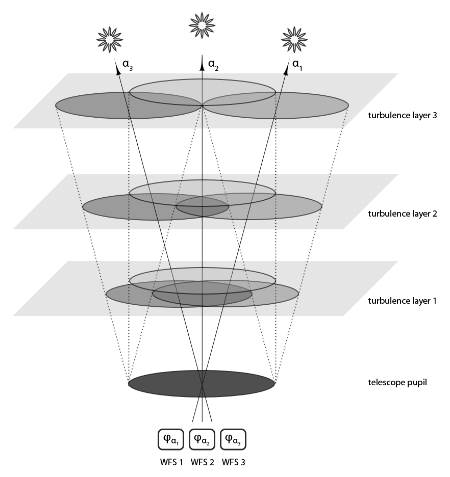
Figure 1. Illustration of the atmospheric tomography problem with three guide star directions, three WFS, and three atmospheric layers.

Current reconstruction algorithms are based on the so-called layered model [34] where the atmosphere is divided into a finite number of slabs or layers (see Fig. 1). The key assumptions are that the turbulence subregions have approximately homogeneous statistics and that each layer is assumed to be statistically independent. A crucial component of all layered models is the refractive index structure parameter (also known as $C_{n}^{2}$-profile or strength profile in telescope imaging literature). The strength profile describes the distribution of the (turbulence) energy in the vertical coordinate. It fluctuates in time and needs to be measured frequently by external instruments.

However, with a change in the strength profile, the discretization (e.g., the number and position of the layers) of the atmosphere in the tomographic reconstructor may become inefficient. As the real-time nature of atmospheric tomography dictates that applicable computational resources are very limited, an optimized model is vital in achieving good imaging quality. This remains an issue as well in the next-generation implementations due to the rapid increase of system sizes. To the knowledge of the authors, no analytical method exists to optimize the discretization with respect to the strength profile.

While the literature on reconstruction methods is well-developed, analytical model optimization has gained less attention: how sensitive are the algorithms to fluctuations in the strength profile? How to choose an optimal model for the atmosphere? In the current generation of telescopes, the turbulence strength profile is measured using independent instruments, e.g., MASS and SCIDAR [26]. The impact of the turbulence strength on the tomographic reconstruction has been studied, e.g., in [16, 11, 18, 12]. Novel numerical methods have been recently proposed for estimating the profile based on the wavefront sensor measurements [19, 10]. Such a method would carry the advantage of integrating the strength profile modelling more closely to the reconstruction algorithm. Nonetheless, the question of choosing an optimal computational model seems open.

In this work we focus on model optimization in atmospheric tomography. We introduce a novel reconstruction method that simultaneously produces an estimate of the turbulent layers as well as the turbulence profile. We show that while such an algorithm requires a comparably large computational effort, it can be qualitatively superior in situations where there is uncertainty in the strength profile. What is more, we present a modification of this method which enforces sparsity on the profile-solution. In other words, the algorithm produces an estimate of the atmosphere which is optimized in both the data fidelity as well as the number and the altitudes of the layers. The ability to do so is the crux of model optimization. Given the computational resources (roughly how many layers can be modeled), our method is able to optimize the model (altitudes of the layers) based on the data-stream.

For the optimization, we propose two alternative procedures, an alternating minimization-type algorithm, which switches between a layer-reconstruction step and a layer-strength identification step and an iterative shrinkage-type method, which promotes a sparse atmosphere model and hence is tailored for model reduction. Although both methods approximate the solution to the same optimization problem, they have different scopes, as we will explain below.

A second major contribution in this paper is to include an additional clustering structure of the layers by grouping them into independent clusters. Such a step is important in view of an intended model reduction because otherwise the predominant ground layer overshadows all other layers.

The results in this paper are demonstrated and confirmed by simulations in an adaptive optics simulation environment called the MOST [3]. Let us mention that for the simulations, we have chosen rather idealistic imaging conditions. Including more practically relevant effects such as spot elongation and tip-tilt indetermination [34] is important if one aims to measure the real-life performance of a reconstruction algorithm. In this work we instead concentrate on the effects taking place in the reconstructed strength profile and how energy is divided to different altitudes. Our objective is to build the basis for such an optimization algorithm.

This paper is organized as follows. In Section 2, we describe the problem setting and review a model for atmospheric turbulence. Section 3 is concerned with a Bayesian approach to the problem of atmospheric tomography. In Section 4, we state several equivalent optimization problems and propose two different algorithms, an alternating minimization procedure and an iterative shrinkage method. Numerical results are presented in Section 5.

2. Problem setting

2.1. Light propagation in the atmosphere

The wind in the atmosphere causes an irregular mixing of warm and cold air. This effect is called the atmospheric turbulence. The fluctuations of the temperature are essentially proportional to the refractive index fluctuations [32], and hence, turbulence affects the propagation of light.

In atmospheric tomography one aims to reconstruct the turbulence profile given wavefront sensor (WFS) measurements. Further, in an AO system, these data are used to adapt the shape of one or more deformable mirrors (DM). Below we assume that the tomography problem (WFS data to atmosphere reconstruction) can be divided into two reliable steps where the incoming wavefronts are resolved in an intermediate stage. Together with the DM shape optimization step, such an approach is sometimes referred to as the 3-step approach [30]. The 3-step approach typically requires good imaging conditions in order to be successful.

In the following, we are mainly interested in the second step, i.e., estimating the atmosphere from the incoming wavefronts (see Fig, 1). Let us therefore explain next the physical model that connects the turbulence layers located at different altitudes $h_{l}$, $l=1,\ldots L$, to the incoming wavefronts $\varphi_{\alpha_{g}}$, $g=1,...,G$, in each guide star direction.

We define the forward operator ${\bf A}$ as the mapping from the atmosphere consisting of $L$ layers to the $G$ incoming wavefronts

(1) $$\begin{split}{\bf A}:\mathop{\raisebox{-2.15277pt}{\hbox{\huge{$\times$}}}}_{l=1}^{L}L^{2}(\Omega_{l})\,\to\,\mathop{\raisebox{-2.15277pt}{\hbox{\huge{$\times$}}}}_{g=1}^{G}L^{2}(\Omega_{D})\,,\\ {\bf A}=:[{\bf A}_{\alpha_{1}},\dots,{\bf A}_{\alpha_{G}}]\,,\end{split}$$

with the operators in guide star directions $\alpha_{g}:=(\alpha_{g}^{(1)},\alpha_{g}^{(2)}),$ corresponding to the 3D directional vector $(\alpha_{g}^{(1)},\alpha_{g}^{(2)},1),$ $g=1,\ldots G.$ Above, $\Omega_{D}$ and $\Omega_{l}$ stand for the layer domains and the telescope aperture, respectively; see (4), (5). A next-generation adaptive optics system typically utilizes a mix of natural guide stars (NGS) and laser guide stars (LGS). For this work, the crucial difference is in the geometry of light propagation explained below.

Under the geometric optics approximation and appropriate assumptions on the atmosphere, the distortions in the phase of light are proportional to the integral over the refractive index fluctuations along the path of light. In the layered model of atmosphere, the precise formula for the forward operator is

(2) $$\begin{split}{\bf A}_{\alpha_{g}}:&\mathop{\raisebox{-2.15277pt}{\hbox{\huge{$\times$}}}}_{l=1}^{L}L^{2}(\Omega_{l})\to L^{2}(\Omega_{D})\,,\\ {\bf A}_{\alpha_{g}}{\boldsymbol{\Phi}}&:=\sum_{l=1}^{L}{\Phi^{(l)}(c_{l}{r}+h_{l}\alpha_{g})}=\varphi_{\alpha_{g}}({r})~{},\,\quad{r}\in\Omega_{D}\,,g=1,\ldots G,\end{split}$$

where $\Phi^{(l)}$ represents the fluctuations of the refractive index (also referred to as “turbulence” in the following) at layer $l$. Here $\alpha_{g}$ corresponds to the 3D directional vector $(\alpha_{g}^{(1)},\alpha_{g}^{(2)},1)$ and $c_{l}$ is a factor needed in the case of laser guide stars. In fact, the conical propagation of light in LGSs requires a scaling factor

(3) $$c_{l}:=\begin{cases}1\,,&\mbox{for NGS}\\ 1-\frac{h_{l}}{h_{LGS}},&\mbox{for LGS and }\,h_{LGS}.\end{cases}$$

Above, $h_{LGS}$ denotes the altitude where the laser beam scatters, i.e., the altitude where the artificial light source is observed. We assume that the telescope aperture is annular with $D>d\geq 0$ and

(4) $$\Omega_{D}:=\{{r}=(x,y)\in{\mathbb{R}}^{2}\,:\,d\leq\hskip 0.86108pt\|r\|\hskip 0.86108pt\leq D\}.$$

In consequence, the visible areas of the atmosphere at layer $l$ can be described as

(5) $$\Omega_{l}:=\bigcup_{g=1}^{G}\Omega_{D}(h_{l}\alpha_{g})\,,\quad\mbox{ with }\,\quad\Omega_{D}(h_{l}\alpha_{g}):=\left\{{r}\in{\mathbb{R}}^{2}\,:\,\frac{{r}-h_{l}\alpha_{g}}{c_{l}}\in\Omega_{D}\right\}\,.$$

Note that it is also possible to consider the tomography operator (2) acting between the spaces $\displaystyle\mathop{\raisebox{-2.15277pt}{\hbox{\huge{$\times$}}}}_{l=1}^{L}H^{1}(\Omega_{l})$ to $H^{1}(\Omega_{D})$; see [14]. Let us explain our notation: we write functions representing turbulence (and only those) at some layer $l$ with an upper bracketed index, $\Phi^{(l)}.$ Moreover, to distinguish between objects on layers and the collection of these objects into a vector, we write the latter as well as all operators acting on these by bold symbols. Thus, the total atmospheric turbulence as the vector having the turbulence at the different layers as entries is expressed as ${\boldsymbol{\Phi}}=(\Phi^{(1)},\ldots,\Phi^{(L)})$.

2.2. Atmospheric turbulence

Statistical models for turbulence are frequently utilized in the AO literature when postulating the tomography step as a Bayesian inference problem. The classical works by Kolmogorov [24] suggest that the turbulence statistics can be modeled by a homogeneous and isotropic Gaussian random field. The key assumption is that the power spectral density satisfies Kolmogorov’s power law, i.e., it is proportional to $|\kappa|^{-11/3}$ for $\ell_{0}\leq\kappa\leq L_{0}$ where $\kappa$ is the spatial frequency of the turbulence field and the bounds $\ell_{0}$ and $L_{0}$ (inner and outer scale, respectively) define the so-called inertial range. Deviations from Kolmogorov turbulence have been debated, but currently Kolmogorov models or variants are commonly used in the reconstruction algorithm literature related to atmospheric tomography.

In this work we assume a so-called von Karman statistics [41] that modifies the Kolmogorov model in order to avoid the singularity at $\kappa=0$. Under the von Karman model, the cumulative turbulence integrated over the atmosphere has a covariance function

(6) $$c_{\Phi}({x}_{1},{x}_{2})=c_{\Phi}(\Delta{x})=\left(\tfrac{L_{0}}{r_{0}}\right)^{\frac{5}{3}}\tfrac{c}{2}\left(\tfrac{2\pi\Delta x}{L_{0}}\right)^{\frac{5}{6}}K_{5/6}\left(\tfrac{2\pi\Delta{x}}{L_{0}}\right)\,,$$

where ${x}_{1},{x}_{2}\in{\mathbb{R}}^{2},$ $\Delta x=|x_{1}-x_{2}|$, the constant $c=\frac{2^{1/6}\Gamma(11/6)}{\pi^{8/3}}\left(\frac{24}{5}\Gamma(\frac{6}{5})\right)^{5/6}$, $K(.)$ is the modified Bessel function of the second type [1], $\Gamma$ is the gamma function, and $r_{0}$ is the Fried parameter [6]. Notice carefully that since $\Phi$ is a stationary random field, the covariance function depends only on the separation of the points ${x}_{1}$ and ${x}_{2}$.

Now let $C_{\Phi}$ denote the covariance operator formally induced by $c_{\Phi}$ in equation (6). We remark that the realizations from the probability distribution of $\Phi$ do not decay at infinity and thus fail to belong to typical function spaces, e.g., $L^{2}({\mathbb{R}}^{2})$. The definition of $C_{\Phi}$ can be made precise as a pseudodifferential operator of order $-11/3$ in weighted Sobolev spaces or using the formalism of generalized random variables [17]. For a detailed expression of $C_{\Phi}$, see [22]. In the following we neglect a more detailed analysis and work with the discretized version of $C_{\Phi}$.

In the layered model of the atmosphere, the cumulative turbulence is decomposed into separate layers by assuming that the a priori distribution of ${\boldsymbol{\Phi}}=(\Phi^{(1)},\ldots,\Phi^{(L)})$ has zero-mean Gaussian statistics with covariance operator ${\rm diag}(\rho_{1}C_{\Phi},...,\rho_{L}C_{\Phi})$, where the relative turbulence strength vector ${\boldsymbol{\rho}}:=(\rho_{1},\ldots\rho_{L})$ is normalized, i.e.,

(7) $$\sum_{l=1}^{L}\rho_{l}=1.$$

Recall that in adaptive optics the cumulative turbulence is typically given from independent measurements and expressed in equation (6). Therefore, the normalization is required for ${\boldsymbol{\rho}}$.

3. The Bayesian approach

In atmospheric tomography one considers the problem

(8) $${\bf A}{\boldsymbol{\Phi}}={\boldsymbol{\varphi}}$$

where ${\boldsymbol{\Phi}}=(\Phi^{(l)})_{l=1}^{L}$ and ${\boldsymbol{\varphi}}=(\varphi_{\alpha_{g}})_{g=1}^{G}$ represent the unknown turbulence layers and incoming wavefronts, respectively, and ${\bf A}$ is given by equation (1). Let us shortly outline how the problem (8) can be interpreted using Bayesian inference.

To avoid technicalities, we assume that the model (8) is discretized by orthogonal projections

$$Q_{m}:\mathop{\raisebox{-2.15277pt}{\hbox{\huge{$\times$}}}}_{l=1}^{L}L^{2}(\Omega_{l})\to X_{m}\subset\mathop{\raisebox{-2.15277pt}{\hbox{\huge{$\times$}}}}_{l=1}^{L}L^{2}(\Omega_{l})\quad{\rm and}\quad R_{n}:\mathop{\raisebox{-2.15277pt}{\hbox{\huge{$\times$}}}}_{g=1}^{G}L^{2}(\Omega_{D})\to Y_{n}\subset\mathop{\raisebox{-2.15277pt}{\hbox{\huge{$\times$}}}}_{g=1}^{G}L^{2}(\Omega_{D}),$$

where the parameters $m,n\in{\mathbb{N}}$ indicate the dimension of each projection, respectively. We set ${\boldsymbol{\varphi}}_{m}=Q_{m}{\boldsymbol{\varphi}}$ and ${\boldsymbol{\Phi}}_{n}=R_{n}{\boldsymbol{\Phi}}$ and obtain a linear system ${\bf A}_{mn}{\boldsymbol{\Phi}}_{n}={\boldsymbol{\varphi}}_{m}$ with ${\bf A}_{mn}=Q_{n}{\bf A}R_{n}$. For this presentation, the details of the discretization basis are not relevant and are omitted.

For the rest of the paper, let us abuse the notation by writing ${\bf A}$, ${\boldsymbol{\Phi}}$ and ${\boldsymbol{\varphi}}$ instead of ${\bf A}_{mn},{\boldsymbol{\Phi}}_{n}$ and ${\boldsymbol{\varphi}}_{m}$ and identify them with matrices and vectors in Euclidean spaces equipped with the Euclidean norm. Hence, in the following, the appearing covariance operators ($C_{\eta}$, $C_{\Phi}$ below) can be represented by non-singular matrices.

Our starting point for the Bayesian setup is based on the splitting of the covariance for ${\boldsymbol{\Phi}}$ into a relative turbulence strength part and a standardized covariance as above. Hence, we assume that the prior model for ${\boldsymbol{\Phi}}$ can be decomposed as

(9) $${\boldsymbol{\Phi}}={\bf W}({\boldsymbol{\rho}})\boldsymbol{\Psi},$$

with two mutually independent random components

(10) $${\bf W}({\boldsymbol{\rho}})={\rm diag}(\sqrt{\rho_{j}})_{j=1}^{L}\in{\mathbb{R}}^{L\times L}\quad\text{ and }\quad\boldsymbol{\Psi}=(\Psi^{(j)})_{j=1}^{L}\,.$$

The vector ${\boldsymbol{\rho}}$ is assumed to be distributed according to

(11) $$\pi_{prior}({{\boldsymbol{\rho}}})\sim\delta_{\Gamma}({\boldsymbol{\rho}}),$$

where $\delta_{\Gamma}$ denotes the Dirac delta on the surface $\Gamma=\{{\boldsymbol{\rho}}\;|\;\sum_{l=1}^{L}\rho_{l}=1,\rho_{l}\geq 0\}\subset{\mathbb{R}}^{L}$. In other words, ${\boldsymbol{\rho}}$ is assumed to be equally distributed within an $L$-dimensional simplex, i.e., we only include the information that it is nonnegative and normalized by (7). Furthermore, we assume $\Psi\sim{\mathcal{N}}(0,\frac{1}{\alpha}{\bf C}_{\Psi})$, where ${\bf C}_{\Psi}={\rm diag}(C_{\Phi},...,C_{\Phi})$ and $\alpha>0$ is the model tuning parameter. We discuss the role of $\alpha$ in more detail below.

In the following, we choose to make statistical inference on the pair $({\boldsymbol{\rho}},\boldsymbol{\Psi})$ instead of ${\boldsymbol{\Phi}}$. Since the two were assumed to be independent, we have

$$\pi_{\rm prior}({\boldsymbol{\rho}},\boldsymbol{\Psi})=\pi_{\rm prior}({\boldsymbol{\rho}})\pi_{\rm prior}(\boldsymbol{\Psi}).$$

Consequently, the posterior takes the following form

$$\pi_{\rm post}({\boldsymbol{\rho}},\boldsymbol{\Psi}\;|\;{\boldsymbol{\varphi}})=c\pi_{\rm prior}({\boldsymbol{\rho}})\pi_{\rm prior}(\boldsymbol{\Psi})\pi_{\rm noise}({\boldsymbol{\varphi}}-{\bf A}{\bf W}({\boldsymbol{\rho}})\boldsymbol{\Psi}),$$

where the constant $c$ depends on the measurement ${\boldsymbol{\varphi}}$. Assuming that the measurement noise is Gaussian to a good approximation with zero mean and covariance matrix $C_{\eta},$ we conclude that the MAP estimate is obtained from a constrained optimization problem

(12) $$\begin{split}(\boldsymbol{\Psi}_{{\rm MAP}},{\boldsymbol{\rho}}_{{\rm MAP}})&\in\operatorname*{arg\,min}_{\begin{subarray}{c}\boldsymbol{\Psi}\in Y_{n}\\ {\boldsymbol{\rho}}\in\Gamma\end{subarray}}\mathcal{K}(\boldsymbol{\Psi},{\boldsymbol{\rho}})\\ \mathcal{K}(\boldsymbol{\Psi},{\boldsymbol{\rho}})&:=\hskip 0.86108pt\|C_{\eta}^{-\frac{1}{2}}({\bf A}{\bf W}({\boldsymbol{\rho}})\boldsymbol{\Psi}-{\boldsymbol{\varphi}})\|\hskip 0.86108pt^{2}_{2}+\alpha\hskip 0.86108pt\|{\bf C}_{\Psi}^{-1/2}\boldsymbol{\Psi}\|\hskip 0.86108pt^{2}_{2}\,.\end{split}$$

Remark 1.

We point out that, in general, a MAP estimate is not invariant under reparametrizations (see e.g. [13]). More precisely, consider the mapping $f:({\boldsymbol{\Phi}},{\boldsymbol{\rho}})\mapsto(\boldsymbol{\Psi},{\boldsymbol{\rho}})$. In our case, the image $f({\boldsymbol{\Phi}}_{MAP},{\boldsymbol{\rho}}_{MAP})$ does not coincide with $(\boldsymbol{\Psi}_{MAP},{\boldsymbol{\rho}}_{MAP})$ since the dependency of ${\boldsymbol{\Phi}}$ and ${\boldsymbol{\rho}}$ will introduce additional non-quadratic terms in the minimization problem (12). Our numerical simulations suggest that the MAP estimator in (12) represents the posterior well and has good approximation properties in practical settings. In addition, the MAP estimate becomes discretization invariant with respect to $\boldsymbol{\Psi}$ [21] and connects directly to an interesting class of optimization problems related to sparse structures. It remains (an important) part of future work to study the posterior from perspective of conditional mean estimates and confidence intervals. These practically motivated objectives are out of the scope of this treatise.

Although not obvious at first sight, the estimator in (12) has a built-in sparsity-enforcing mechanism. In practice, when the dimension of the data is radically lower than the unknown, such a method yields an estimate ${\boldsymbol{\rho}}_{{\rm MAP}}$ which has zero turbulence strength at several altitudes. This contradicts with reality in the sense that the turbulence profile is considered smooth with respect to the altitude. However, we will demonstrate below that decreasing the dimension (fewer layers are used in the model) reduces or even removes the sparsity effect.

For a higher number of layers, our simulations suggest that the solution is optimal under a constraint that a fixed number of turbulence strength components $\rho_{l}$ are non-zero. Let us make this claim more precise: suppose we model $L$ layers. Then the solution $(\Psi_{MAP},{\boldsymbol{\rho}}_{{\rm MAP}})$ in (12) has $L_{0}$ non-zero components $\rho_{l}$ for some $L_{0}\leq L$. Moreover, $(\Psi_{MAP},{\boldsymbol{\rho}}_{{\rm MAP}})$ is optimal (in the sense of minimizing the functional $\mathcal{K}$) among all reconstructions that have only $L_{0}$ non-zero layers (out of the chosen set of $L$ layers). What is more, we can control the number $L_{0}$ by adjusting the regularization term in (12) by tuning $\alpha$.

Below we find that in such an approach the layers at lower altitudes become heavily preferred. This is due to both geometrical factors as well as the fact that most of the turbulence is located close to the ground. For a more detailed analysis, see Section 5. In order to include layers at higher altitude to the solution we introduce additional information. We assume that we know the cumulative turbulence strength on some altitude intervals in the atmosphere. In a nutshell, the set of layers is divided into clusters of layers and we know the cumulative strength over each cluster.

Let us discuss the clustering in more detail. We assume that $N<L$ clusters, ${\mathcal{B}}_{1},\dots,{\mathcal{B}}_{N}$, are given which constitute a partition of the layers, i.e.,

(13) $${\mathcal{B}}_{i}\subset\{1,\ldots,L\},\quad\bigcup_{i=1}^{N}\mathcal{B}_{i}=\{1,\ldots,L\},\quad{\mathcal{B}}_{i}\cap\mathcal{B}_{j}=\emptyset\text{ for }i\neq j,$$

and on each cluster we fix a total turbulent energy $d_{i}$ as

(14) $$d_{i}:=\sum_{l\in{\mathcal{B}}_{i}}\rho_{l},\qquad{\bf d}:=(d_{1},\ldots,d_{N}),\qquad\sum_{i=1}^{N}d_{i}=1\,,$$

where ${\bf d}$ is given. Further, we assume that the prior is uniformly distributed on the simpleces formed by the clusters ${\mathcal{B}}_{j}$ in the following way

(15) $$\pi_{\rm prior}({{\boldsymbol{\rho}}})\sim\delta_{\Gamma_{N}},$$

where

$$\Gamma_{N}({\bf d})=\left\{{\boldsymbol{\rho}}\in{\mathbb{R}}^{L}\Big{|}\;\sum_{l\in{\mathcal{B}}_{i}}\rho_{l}=d_{i}\textrm{ for all }i=1,...,N,\rho_{l}\geq 0,l=1,\ldots L\right\}.$$

Including this additional information we propose now a modified method with an a priori fixed vector ${\bf d}$ such that the MAP estimate is given analogous to (12) by

(16) $$(\boldsymbol{\Psi}_{{\rm MAP}},{\boldsymbol{\rho}}_{{\rm MAP}})\in\operatorname*{arg\,min}_{\begin{subarray}{c}\boldsymbol{\Psi}\in Y_{n}\\ {\boldsymbol{\rho}}\in\Gamma_{N}({\bf d})\end{subarray}}\mathcal{K}(\boldsymbol{\Psi},{\boldsymbol{\rho}}),$$

with $\mathcal{K}(\boldsymbol{\Psi},{\boldsymbol{\rho}})$ as in (12). Obviously, the modified method reduces to the original by setting $N=1$.

Let us now return to the role of parameter the $\alpha$. As mentioned above, the constraint ${\boldsymbol{\rho}}\in\Gamma_{N}$ enforces some sparsity on the solution. This phenomenon is illustrated in Proposition 2 in more clarity. Moreover, we notice that the parameter $\alpha$ controls how sparse the obtained solutions are. From a Bayesian point of view, $\alpha$ defines the subjective demand for model reduction. The parameter $\alpha$ can also be interpreted otherwise: consider two problems with parameters $\alpha$ and $\alpha^{\prime}$. It is straightforward to see that the problem (16) with $\alpha$ is equivalent to a situation where $\alpha^{\prime}=1$, but where $\Gamma_{N}^{\prime}$ is normalized to $1/\alpha$, i.e., $\sum_{i=1}^{N}d_{i}^{\prime}=1/\alpha$. The intuition is that a large $\alpha$ artificially enforces a lower cumulative strength in order to achieve economically a reasonable model fit. In Section 5 we explore the proposed method with various choices of $\alpha$.

4. Optimization problems and algorithms

4.1. The maximum a posteriori estimate revisited

In this section we study problem (16), rewrite it into alternative forms, and discuss algorithms to solve it. We propose two different algorithms, namely an alternating minimization procedure and an iterative shrinkage method based on eliminating the strength vector ${\boldsymbol{\rho}}$.

Proposition 1.

The optimization problem (16) is equivalent to the problem

(17) $$\begin{split}({\boldsymbol{\Phi}}_{{\rm MAP}},{\boldsymbol{\rho}}_{{\rm MAP}})&\in\operatorname*{arg\,min}_{\begin{subarray}{c}{\boldsymbol{\Phi}}\in Y_{n}\\ {\boldsymbol{\rho}}\in\Gamma_{N}({\bf d})\\ {\bf W}({\boldsymbol{\rho}})^{\dagger}{\bf W}({\boldsymbol{\rho}}){\boldsymbol{\Phi}}={\boldsymbol{\Phi}}\end{subarray}}\mathcal{F}({\boldsymbol{\Phi}},{\boldsymbol{\rho}})\\ \mathcal{F}({\boldsymbol{\Phi}},{\boldsymbol{\rho}})&:=\hskip 0.86108pt\|C_{\eta}^{-\frac{1}{2}}({\bf A}{\boldsymbol{\Phi}}-{\boldsymbol{\varphi}})\|\hskip 0.86108pt^{2}_{2}+\alpha\hskip 0.86108pt\|{\bf C}_{\Psi}^{-1/2}{\bf W}({\boldsymbol{\rho}})^{\dagger}{\boldsymbol{\Phi}}\|\hskip 0.86108pt^{2}_{2},\end{split}$$

where ${\bf W}({\boldsymbol{\rho}})^{\dagger}$ denotes the Moore-Penrose pseudoinverse,

$${\bf W}({\boldsymbol{\rho}})^{\dagger}={\rm diag}\left(\begin{cases}\frac{1}{\sqrt{\rho_{j}}}&\text{ if }\rho_{j}>0,\\ 0&\text{ else }\end{cases}\right)_{j=1}^{L}\in{\mathbb{R}}^{L\times L}.$$

More precisely, equivalence holds in the following sense: if $({\boldsymbol{\rho}}_{{\rm MAP}},\boldsymbol{\Psi}_{{\rm MAP}})$ solves (16), then $({\boldsymbol{\rho}}^{\prime}_{{\rm MAP}},{\boldsymbol{\Phi}}_{{\rm MAP}}):=({\boldsymbol{\rho}}_{{\rm MAP}},{\bf W}({\boldsymbol{\rho}})\boldsymbol{\Psi}_{{\rm MAP}})$ solves (17), and if $({\boldsymbol{\rho}}^{\prime}_{{\rm MAP}},{\boldsymbol{\Phi}}_{{\rm MAP}})$ solves (17), then $({\boldsymbol{\rho}}_{{\rm MAP}},\boldsymbol{\Psi}_{{\rm MAP}}):=({\boldsymbol{\rho}}^{\prime}_{{\rm MAP}},{\bf W}({\boldsymbol{\rho}}^{\prime}_{{\rm MAP}})^{\dagger}{\boldsymbol{\Phi}}_{{\rm MAP}})$ solves (16).

Proof.

Let $({\boldsymbol{\rho}}_{{\rm MAP}},\boldsymbol{\Psi}_{{\rm MAP}})$ solve (16). Let ${\mathcal{I}}=\{i\,|\,({\boldsymbol{\rho}}_{{\rm MAP}})_{i}=0\}$ be the zero indices of ${\boldsymbol{\rho}}_{{\rm MAP}}$. Since $(\Psi_{{\rm MAP}}^{(i)})_{i\in{\mathcal{I}}}$ do not contribute to the first term in (16) and the second term is a sum of squares over the layers, it follows by the minimization property that the corresponding entries in $\boldsymbol{\Psi}$ must vanish: $(\Psi_{{\rm MAP}}^{(i)})_{i\in{\mathcal{I}}}=0.$ Therefore, problem (16) is equivalent to the same optimization problem with the additional constraint ${\bf W}({\boldsymbol{\rho}})^{\dagger}{\bf W}({\boldsymbol{\rho}})\boldsymbol{\Psi}=\boldsymbol{\Psi}$. Hence, by setting ${\boldsymbol{\Phi}}_{{\rm MAP}}:={\bf W}({\boldsymbol{\rho}})\boldsymbol{\Psi}_{{\rm MAP}},$ we arrive at (17) with the additional constraint that there exists a $\boldsymbol{\Psi}$ with ${\boldsymbol{\Phi}}={\bf W}({\boldsymbol{\rho}})\boldsymbol{\Psi}$ and ${\bf W}({\boldsymbol{\rho}})^{\dagger}{\boldsymbol{\Phi}}=\boldsymbol{\Psi}$. It is a simple calculation that this constraint is satisfied if and only if ${\bf W}({\boldsymbol{\rho}})^{\dagger}{\bf W}({\boldsymbol{\rho}}){\boldsymbol{\Phi}}={\boldsymbol{\Phi}}.$ The same argument reversed implies that solutions to (17) yield corresponding solutions to (16). ∎

Next, we eliminate the strength vector ${\boldsymbol{\rho}}$ from the optimization problem by minimizing over it.

Proposition 2.

Let $({\boldsymbol{\Phi}}_{{\rm MAP}},{\boldsymbol{\rho}}_{{\rm MAP}})\in Y_{n}\times\Gamma_{N}({\bf d})$ be minimizers of (17) for some ${\bf d}>0$. Then ${\boldsymbol{\Phi}}_{{\rm MAP}}$ is also a solution of the optimization problem

(18) $$\begin{split}{\boldsymbol{\Phi}}_{{\rm MAP}}&=\operatorname*{arg\,min}_{{\boldsymbol{\Phi}}\in Y_{n}}\mathcal{G}({\boldsymbol{\Phi}}),\\ \mathcal{G}({\boldsymbol{\Phi}})&:=\hskip 0.86108pt\|C_{\eta}^{-\frac{1}{2}}({\bf A}{\boldsymbol{\Phi}}-{\boldsymbol{\varphi}})\|\hskip 0.86108pt^{2}_{2}+\alpha\sum_{i=1}^{N}\frac{1}{d_{i}}\left(\sum_{l\in{\mathcal{B}}_{i}}\hskip 0.86108pt\|C_{\Phi}^{-1/2}\Phi^{(l)}\|\hskip 0.86108pt\right)^{2},\end{split}$$

where $d_{i}$ are as in equation (14). If for some cluster ${\mathcal{B}}_{i},$ the vector $({\boldsymbol{\Phi}}_{{\rm MAP}}^{(l)})_{l\in{\mathcal{B}}_{i}}$ is non-zero, the $l$-th component of the strength vectors at this cluster, $({\boldsymbol{\rho}}_{{\rm MAP}})_{l},$ is uniquely defined by

(19) $$\qquad({\boldsymbol{\rho}}_{{\rm MAP}})_{l}=d_{i}\frac{\hskip 0.86108pt\|C_{\Phi}^{-1/2}\Phi_{{\rm MAP}}^{(l)}\|\hskip 0.86108pt}{\sum_{l\in{\mathcal{B}}_{i}}\hskip 0.86108pt\|C_{\Phi}^{-1/2}\Phi_{{\rm MAP}}^{(l)}\|\hskip 0.86108pt},\quad\forall l\in{\mathcal{B}}_{i}.$$

Proof.

With ${\boldsymbol{\Phi}}_{{\rm MAP}}$ a solution to (17), we can compare the function values of $({\boldsymbol{\Phi}}_{{\rm MAP}},{\boldsymbol{\rho}}_{{\rm MAP}})$ with all admissible values for $({\boldsymbol{\Phi}}_{{\rm MAP}},{\boldsymbol{\rho}}),$ i.e., where ${\boldsymbol{\rho}}$ satisfies the constraints ${\boldsymbol{\rho}}\in\Gamma_{N}({\bf d})$ and $\rho_{l}>0$ whenever $\Phi_{{\rm MAP}}^{(l)}\not=0.$ Since ${\boldsymbol{\rho}}_{{\rm MAP}}$ must be minimal, it follows that

$${\boldsymbol{\rho}}_{{\rm MAP}}\in\operatorname*{arg\,min}_{{\boldsymbol{\rho}}\in\Gamma_{n}({\bf d})}\sum_{i=1}^{N}\sum_{l\in{\mathcal{B}}_{i},\Phi^{(l)}\not=0}\frac{1}{\rho_{l}}\hskip 0.86108pt\|C_{\Phi}^{-1/2}\Phi_{{\rm MAP}}^{(l)}\|\hskip 0.86108pt^{2}$$

since the first term in (17) does not depend on ${\boldsymbol{\rho}}$. This optimization problem can be solved yielding (19) for those clusters ${\mathcal{B}}_{i}$ where $\Phi_{{\rm MAP}}^{(l)}$ is not all zero for $l\in{\mathcal{B}}_{i}$. For the other clusters the functional value and the constraints are independent of the strength vector on these clusters, hence $({\boldsymbol{\rho}}_{{\rm MAP}})_{l}$ can be arbitrary with the only restriction that $\sum_{l\in{\mathcal{B}}_{k}}\rho_{l}=d_{k}$ on these clusters. By plugging in the formula for ${\boldsymbol{\rho}}_{{\rm MAP}}$ in (19) into the functional in (17), we find that its optimal value is that of $\mathcal{G}({\boldsymbol{\Phi}}_{{\rm MAP}})$ in (18). Conversely, for any ${\boldsymbol{\Phi}}$, we can construct a ${\boldsymbol{\rho}}$ as given in (19) such that $\mathcal{G}({\boldsymbol{\Phi}})$ equals $\mathcal{F}({\boldsymbol{\Phi}},{\boldsymbol{\rho}})$ in (17). Thus, it follows that ${\boldsymbol{\Phi}}_{{\rm MAP}}$ must be a minimizer of $\mathcal{G}$ as well and this proves the proposition. ∎

From these results we can study existence and uniqueness of minimizers of the functionals above.

Proposition 3.

Let $\alpha,{\bf d}>0$, matrices ${\bf C}_{\Psi}$ and $C_{\eta}$ be positive definite and $({\boldsymbol{\Phi}},{\boldsymbol{\rho}})\in Y_{n}\times\Gamma_{N}({\bf d}).$ Then problems (16), (17) and (18) have minimizers. The minimizer ${\boldsymbol{\Phi}}_{{\rm MAP}}$ in (17) and (18) is unique and ${\boldsymbol{\rho}}_{{\rm MAP}}$ is unique at a cluster ${\mathcal{B}}_{i}$ if $({\boldsymbol{\Phi}}_{{\rm MAP}}^{(l)})_{l\in{\mathcal{B}}_{i}}\not=0.$

Proof.

Since the problem is finite dimensional, it follows by straightforward argumentation that (16) has a solution. Note that the functional $\mathcal{K}$ is continuous in both arguments. By Propositions 1, 2 the same holds for (17) and (19). The functional $\mathcal{G}$ in (18) is strictly convex in ${\boldsymbol{\Phi}}$, thus the minimizer ${\boldsymbol{\Phi}}_{{\rm MAP}}$ is unique, by formula (19), ${\boldsymbol{\rho}}_{{\rm MAP}}$ is unique if ${\boldsymbol{\Phi}}_{{\rm MAP}}$ is not all zero at a cluster. ∎

The reduced problem (18) can be interpreted as a regularization with penalty term being of the type of an $l^{1}$-norm squared. It is well-known that such a penalty enforces sparsity, i.e., solutions to (17) will lead to a ${\boldsymbol{\Phi}}$ that vanishes on many layers (if the real ${\boldsymbol{\Phi}}$ is sparse and $\alpha$ is sufficiently large). This is the reason why (12) ($L=1$) is not appropriate, because the corresponding estimator usually has only values on very few layers, which is not how a real atmosphere behaves. The introduction of the clustering structure of the layers and the weights ${\bf d}$ allows for more flexibility and “sparsifies” less, depending on the weights.

4.2. Alternating Minimization Algorithm

In Proposition 2 we calculated the minimizers with respect to ${\boldsymbol{\rho}},$ when ${\boldsymbol{\Phi}}$ is given. This suggests to apply an alternating minimization procedure for solving (17), where the approximate solutions ${\boldsymbol{\Phi}}_{k},{\boldsymbol{\rho}}_{k},$ $k=1,\ldots$ are defined iteratively as

(20) $${\boldsymbol{\Phi}}_{k+1}:=\operatorname*{arg\,min}_{\begin{subarray}{c}{\boldsymbol{\Phi}}\in Y_{n},\\ {\bf W}({\boldsymbol{\rho}}_{k})^{\dagger}{\bf W}({\boldsymbol{\rho}}_{k}){\boldsymbol{\Phi}}={\boldsymbol{\Phi}}\end{subarray}}\mathcal{F}({\boldsymbol{\Phi}},{\boldsymbol{\rho}}_{k})\qquad{\boldsymbol{\rho}}_{k+1}:=\operatorname*{arg\,min}_{{\boldsymbol{\rho}}\in\Gamma_{N}({\bf d})}\mathcal{F}({\boldsymbol{\Phi}}_{k+1},{\boldsymbol{\rho}}_{k}).$$

Note that ${\boldsymbol{\rho}}_{k+1}$ can be computed explicitly by (19) (taking special care in case of ${\boldsymbol{\Phi}}$ being zero at a cluster). For numerical calculations, the evaluation of ${\bf W}({\boldsymbol{\rho}})^{\dagger}$ is problematic as it can lead to numerical overflow if ${\boldsymbol{\rho}}$ has very small entries. A not uncommon remedy is to regularize ${\bf W}$ to prevent it becoming near singular. Thus, we approximate problem (17) by adding a small value $\epsilon$ to $\rho_{l}$ in ${\bf W},$ i.e., ${\bf W}_{\epsilon}({\boldsymbol{\rho}}):={\bf W}({\boldsymbol{\rho}}+\epsilon)$ is used in place of ${\bf W}({\boldsymbol{\rho}})$. This has the additional effect that the constraint ${\bf W}({\boldsymbol{\rho}})^{\dagger}{\bf W}({\boldsymbol{\rho}}){\boldsymbol{\Phi}}={\boldsymbol{\Phi}}$ is trivially fulfilled and can be dropped.

The computation of ${\boldsymbol{\Phi}}_{k+1}$ involves then a quadratic optimization problem, hence, ${\boldsymbol{\Phi}}_{k+1}$ is given as solution to the optimality conditions

(21) $$\left({\bf A}^{T}C_{\eta}^{-1}{\bf A}+\alpha\cdot{\bf P}({\boldsymbol{\rho}}_{k})^{-1}{\bf C}_{\Psi}^{-1}\right){\boldsymbol{\Phi}}_{k+1}={\bf A}^{T}C_{\eta}^{-1}{\boldsymbol{\varphi}},.$$

with

(22) $${\bf P}({\boldsymbol{\rho}})^{-1}:={{\bf W}_{\epsilon}({\boldsymbol{\rho}})^{*}}^{\dagger}{\bf W}_{\epsilon}({\boldsymbol{\rho}})^{\dagger}=\mbox{diag}(\tfrac{1}{\rho_{l}+\epsilon})_{l=0}^{L}.$$

However, as this system is usually of large scale, we modify this step and compute ${\boldsymbol{\Phi}}_{k+1}$ in (21) by an approximate minimization using a finite number of steps of an iterative procedure like a gradient method. The resulting algorithm reads as follows:

Algorithm 1 Alternating Minimization Algorithm in Blocks of Layers

Parameter: $\alpha,{\bf d}>0$, INNER, the number of inner gradient iterations, ${\bf C}_{\Psi}^{-1},$ $C_{\eta}^{-1},$ and a sequence of stepsizes $(\tau_{i})_{k}$ and initial guesses ${\boldsymbol{\rho}}_{\rm init},{\boldsymbol{\Phi}}_{\rm init}.$ Set ${\boldsymbol{\rho}}_{1}={\boldsymbol{\rho}}_{\rm init}$, ${\bf P}({\boldsymbol{\rho}}_{1})$ as in (22), ${\boldsymbol{\Phi}}_{1,0}={\boldsymbol{\Phi}}_{\rm init}.$

for $i=1,\dots$ until convergence  do

     for $k=1,\dots\text{INNER}$ do $\triangleright$ perform one or several steps of a gradient method

         ${\boldsymbol{\Phi}}_{i,k}={\boldsymbol{\Phi}}_{i,k-1}+\tau_{i,k-1}\left({\bf A}^{\ast}C_{\eta}^{-1}({\boldsymbol{\varphi}}-{\bf A}{\boldsymbol{\Phi}}_{i,k-1})-\alpha\cdot{\bf P}({\boldsymbol{\rho}}_{i})^{-1}{\bf C}_{\Psi}^{-1}{\boldsymbol{\Phi}}_{i,k-1}\right)$

     end for

     ${\boldsymbol{\Phi}}_{i+1,0}:={\boldsymbol{\Phi}}_{i,k}$

     for $n=1,\dots,N$ do

         for $l\in{\mathcal{B}}_{n}\ \textbf{do}$

              $\rho_{l}=d_{n}\cdot\hskip 0.86108pt\|C_{\Phi}^{-1/2}\Phi_{i,k}^{(l)}\|\hskip 0.86108pt\Big{/}\displaystyle\sum_{l\in{\mathcal{B}}_{n}}\hskip 0.86108pt\|C_{\Phi}^{-1/2}\Phi_{i,k}^{(l)}\|\hskip 0.86108pt$ $\triangleright$ update turbulence weights

         end for

     end for

     ${\boldsymbol{\rho}}_{i+1}:=(\rho_{1},\ldots,\rho_{N}).$

end for

In Algorithm 1, several implementation details are left out for simplicity. Of course, a standard convergence criterion for the outer loop is required. The parameter INNER defines the number of inner iterations. If formally $\text{INNER}=\infty$ (and assuming the gradient method converges), then we obtain the exact alternating minimization in (20). We preset the parameter INNER to a fixed value as described below. The sequence of stepsizes $\tau_{k}$ can be chosen constant with the standard convergence constraint $\tau_{k}<\lambda_{\max}({\bf A}^{\ast}C_{\eta}^{-1}{\bf A}).$ However, we allow for more advanced non-constant stepsizes as well.

Despite its deficiencies, the alternating minimization algorithm has one big advantage over other methods like those that minimize problem (16): it is rather simple, and most important, it can be included easily into existing software. In fact, the inner iteration with the iteration variable $k$ for ${\boldsymbol{\Phi}}_{k}$ is exactly a standard gradient method for the atmospheric tomography problem when the turbulence strength is known as it is commonly used in AO. From the aspect of implementation, if a standard atmospheric tomography solver is already available, then the only additional procedure, namely calculating ${\boldsymbol{\rho}}$, is straightforward, and thus the alternating minimization method is a convenient choice. In particular, this applies to the dynamic (time-dependent) reconstruction problem, where the method can be easily adapted to.

Let us remark on the convergence of Algorithm 1. Such alternating minimization procedures are well-known and can be viewed as nonlinear variants of Gauss-Seidel iterations. A convergence proof (limit points of the sequence are stationary points) in the discretized (i.e., finite-dimensional case) can, e.g., be found in [7, Proposition 2.7.1] and the references therein. Note, however, that for general functionals the alternating procedure does not have to converge, as it was shown by a counterexample of Powell [29]. The cited convergence result in [7] applies to our case if we restrict the problem to having all positive strength ${\boldsymbol{\rho}}\geq\epsilon>0$ (with a small parameter $\epsilon$, e.g., of the order of machine epsilon). Using these results and the positivity restriction (which is just another way of introducing a regularization of ${\bf P}({\boldsymbol{\rho}})^{-1}$ similar to (22)) it can be concluded that then the exact iteration in (20) converges to the unique minimum.

We also mention that the transformation of problem (16) to problem (17) and the associated algorithms have also been applied in other contexts like in variational image processing for nondifferentiable penalty functionals, e.g., for the ROF-functional. There the corresponding alternating minimization method is known under the name of half-quadratic minimization [2, Section 3.2.4], [9] and also by the name of iteratively reweighted minimization [33].

According to Proposition 1, the two optimization problems (12) and (16) are equivalent and a similar alternating minimization algorithm for (12) can be designed. Since (16) arises from a change of variables, it is not surprising that the corresponding iteration for ${\boldsymbol{\Phi}}_{i,k}$ is similar to that in Algorithm 1 but where the gradient direction is preconditioned by ${\bf P}({\boldsymbol{\rho}}_{i}).$ The reason why we prefer (16) over (12) is again the compatibility with existing code for the reconstruction of atmospheric turbulence, where usually ${\boldsymbol{\Phi}}$ is used as the unknown and not $\boldsymbol{\Psi}$.

In the next section we discuss an algorithm for solving (17). As we will see, it does not require an $\epsilon$-regularization of ${\bf W}$ and is hence more robust for the case of layers with vanishing strength $\rho_{i}=0$. It looses, however, the implementational benefit of Algorithm 1 of the compatibility with existing code.

4.3. Iterative shrinkage-thresholding algorithm

The second algorithm for solving (17) is based on $\mathcal{G}$ defined in (18), which includes a nondifferentiable term (the $l^{1}$-norm squared). In particular, classical derivative-based method cannot be applied, but tools from convex analysis have to be employed. The functional $\mathcal{G}({\boldsymbol{\Phi}})$ can be split into two parts, a quadratic one $f$ and a convex nondifferentiable one $g$:

(23) $$\mathcal{G}({\boldsymbol{\Phi}})=f({\boldsymbol{\Phi}})+g({\boldsymbol{\Phi}})\,.$$

There is an arsenal of methods to tackle the corresponding optimization problems, for instance, primal-dual algorithms [44], augmented Lagrangian methods [23, 28], Alternating Direction Method of Multipliers [8], Bregman [27] and split Bregman [20] methods, just to mention a few.

Since we want a simple yet efficient one, we propose to use the iterative shrinkage-thresholding algorithm (ISTA) of Beck and Teboulle [5] together with its accelerated version FISTA. ISTA is defined as follows: a parameter $\lambda$ is fixed, which is set to be larger than the Lipschitz constant of $f$. In ISTA, a sequence of iterations ${\boldsymbol{\Phi}}_{k}$ for minimizing (23) is defined as

$${\boldsymbol{\Phi}}_{k+1}: =\text{prox}_{\lambda^{-1}}({\boldsymbol{\Phi}}_{k}-\tfrac{1}{\lambda}\nabla f({\boldsymbol{\Phi}}_{k})),\qquad\text{where}$$

$$\text{prox}_{\lambda^{-1}}({\bf u}) :=\operatorname*{arg\,min}_{{\bf v}}g({\bf v})+\tfrac{\lambda}{2}\|{\bf u}-{\bf v}\|^{2}.$$

The function $\text{prox}_{\lambda^{-1}}$ is called the proximal mapping. The efficiency of the method is based on the fact that the proximal mapping can often be calculated analytically. In case of $g$ being the $l^{1}$-norm, it amounts to applying a simple soft-shrinkage operator. Thus, to employ ISTA, we have to calculate the proximal mapping associated to the last term in (18). In order to do so, we first rewrite the optimization problem by a change of variables

(24) $$\Theta^{(l)}:=C_{\Phi}^{-1/2}\Phi^{(l)}\quad\Longleftrightarrow\quad\Phi^{(l)}=C_{\Phi}^{1/2}\Theta^{(l)},\qquad\quad l=1,\ldots,L.$$

In the new variables, problem (18) reads as

(25) $$\boldsymbol{\Theta}=\operatorname*{arg\,min}_{\boldsymbol{\Theta}}\tilde{\mathcal{G}}(\boldsymbol{\Theta}),\quad\tilde{\mathcal{G}}(\boldsymbol{\Theta}):=\mathcal{G}\left({\bf C}_{\Psi}^{1/2}\boldsymbol{\Theta}\right),\quad\tilde{\mathcal{G}}(\boldsymbol{\Theta})=\tilde{f}(\boldsymbol{\Theta})+\tilde{g}(\boldsymbol{\Theta})$$

where

$$\tilde{f}(\boldsymbol{\Theta}):=\hskip 0.86108pt\|C_{\eta}^{-1}\left({\bf A}{\bf C}_{\Psi}^{1/2}\boldsymbol{\Theta}-{\boldsymbol{\varphi}}\right)\|\hskip 0.86108pt^{2}_{2}\quad{\rm and}\quad\tilde{g}(\boldsymbol{\Theta}):=\alpha\sum_{i=1}^{L}\frac{1}{d_{i}}\left(\sum_{l\in{\mathcal{B}}_{i}}\hskip 0.86108pt\|\Theta^{(l)}\|\hskip 0.86108pt\right)^{2}.$$

Clearly the minimizers of $\mathcal{G}$ and $\tilde{\mathcal{G}}$ are related by (24). The proximal mapping for $\tilde{g}$ is now separable over the clusters,

$$\text{prox}_{\lambda^{-1}}({\bf u})=\operatorname*{arg\,min}_{{\bf v}=(v^{(1)},\ldots,v^{(L)})}\sum_{i=1}^{L}\left[\tfrac{\alpha}{d_{i}}\left(\sum_{l\in{\mathcal{B}}_{i}}\|{v}^{(l)}\|\right)^{2}+\tfrac{\lambda}{2}\sum_{l\in{\mathcal{B}}_{i}}\|{u}^{(l)}-{v}^{(l)}\|^{2}\right],$$

such that ${v}^{(l)}$ can be computed clusterwise independently. The minimizer of the functional inside the brackets can be found explicitly; see, e.g., [38]. It involves a soft-thresholding within each cluster with threshold parameters $\gamma_{m}$, ${m}=1,\ldots N$,

$$\text{prox}_{\lambda^{-1}}(\boldsymbol{\Psi})=\max\left\{\Psi^{(l)}-\gamma_{m},0\right\}\cdot\frac{\Psi^{(l)}}{\|\Psi^{(l)}\|},\quad\forall l\in{\mathcal{B}}_{m},{m}=1,\ldots,N,$$

and $\gamma_{m}$ is calculated by the following algorithm, which we state in the variables $\Phi^{(l)}=C_{\Phi}^{1/2}\Theta^{(l)}$ for later reference.

Algorithm 2 Proximal mapping threshold parameter

Input: ${\boldsymbol{\Phi}}_{k}$, $C_{\Phi}$, $\alpha,$ $\lambda$, $d_{m},$ ${m}\in\{1,\ldots N\}$

for ${m}=1,\dots,N$ do

     for $l\in{\mathcal{B}}_{m}\ \textbf{do}$

         Compute norms ${\bf n}\in{\mathbb{R}}^{|{\mathcal{B}}_{m}|}$, with ${\bf n}=\left(\hskip 0.86108pt\|C_{\Phi}^{-\frac{1}{2}}{\boldsymbol{\Phi}}^{(l)}_{k}\|\hskip 0.86108pt\right)_{l\in{\mathcal{B}}_{m}}$

     end for

     Sort norms ${\bf\tilde{n}}=\mbox{sort}({\bf n})$ with $\tilde{n}_{1}>\dots>\tilde{n}_{|{\mathcal{B}}{{m}}|}$

     Compute $l^{\ast}:=\max\left\{l\in\{1,\dots,|{\mathcal{B}}_{{m}}|\}:\tilde{n}_{l}-\frac{2\frac{\alpha}{\lambda d_{m}}}{1+2l\frac{\alpha}{\lambda d_{m}}}\sum_{j=1}^{l}\tilde{n}_{j}>0\right\}$

     $\gamma_{m}=\frac{2\frac{\alpha}{\lambda d_{m}}}{1+2l^{\ast}\frac{\alpha}{\lambda d_{m}}}\sum_{j=1}^{l^{\ast}}\tilde{n}_{j}$

end forOutput: $(\gamma_{1},\ldots,\gamma_{N})$

We apply the ISTA iteration to $\tilde{\mathcal{G}},$ yielding a sequence $\boldsymbol{\Psi}_{k}$. Upon a substitution to the original variables $\Phi_{k}^{(l)}=C_{\Phi}^{1/2}\Psi_{k}^{(l)},$ we end up with the following Algorithm 3. Here we also include the possibility to have several inner gradient iterations with respect to $f,$ and the stepsize $\frac{1}{\lambda}$ is fixed such that

(26) $$\lambda>\lambda_{\max}({\bf A}^{\ast}C_{\eta}^{-1}{\bf A}).$$

Algorithm 3 ISTA

Input: $\lambda>0$, $\alpha,{\bf d}>0$, ${\bf C}_{\Psi}^{-1},$ $C_{\eta}^{-1}$, initial guess ${\boldsymbol{\Phi}}_{\rm init}$

Set ${\boldsymbol{\rho}}={\boldsymbol{\rho}}_{\rm init}$, ${\boldsymbol{\Phi}}_{1,0}={\boldsymbol{\Phi}}_{\rm init}$

for $i=1,\dots,$ until convergence  do

     for $k=1,\dots,$ INNER do $\triangleright$ perform one or several steps of a gradient method

         ${\boldsymbol{\Phi}}_{i,k}={\boldsymbol{\Phi}}_{i,k-1}+\frac{1}{\lambda}\cdot{\bf C}_{\Psi}\left({\bf A}^{\ast}C_{\eta}^{-1}({\boldsymbol{\varphi}}-{\bf A}{\boldsymbol{\Phi}}_{i,k-1})\right)$

     end for

     Calculate threshold $\gamma_{m}$ for ${m}=1,\ldots,N$ via Algorithm 2 with ${\boldsymbol{\Phi}}_{i,k}$

     $\Phi_{i,k}^{(l)}=\max\left(\hskip 0.86108pt\|C_{\Phi}^{-1/2}\Phi_{i,k}^{(l)}\|\hskip 0.86108pt-\gamma_{m},0\right)\cdot\frac{\Phi_{i,k}^{(l)}}{\hskip 0.60275pt\|C_{\Phi}^{-1/2}\Phi_{i,k}^{(l)}\|\hskip 0.60275pt},\quad\forall l\in{\mathcal{B}}_{m},{m}=1,\ldots,N$ $\triangleright$ shrinkage

     Set ${\boldsymbol{\Phi}}_{i+1,0}={\boldsymbol{\Phi}}_{i,k}$

end for

Output: ${\boldsymbol{\Phi}}_{i,k}$

The original version of ISTA has $\text{INNER}=1.$ Note that this algorithm has no problem if $\hskip 0.86108pt\|C_{{\boldsymbol{\Phi}}^{(l)}}^{-1/2}{\boldsymbol{\Phi}}_{i,k}^{(l)}\|\hskip 0.86108pt=0$ as the threshold is then simply set to $0$ in the shrinkage step. As before, the turbulence strength weights ${\boldsymbol{\rho}}$ can be found in any outer iteration step by formula (19).

In order to accelerate convergence of ISTA, a fast iterative shrinkage-thresholding algorithm (FISTA) has been introduced in [5]. The method is very similar to ISTA except that it involves a two-step procedure (or alternatively two iteration variables). Only the iteration for ${\boldsymbol{\Phi}}$ is altered while the shrinkage step stays the same. The algorithm exhibits a similar computational cost per iteration than ISTA, but is faster in general. There is no problem in applying the FISTA acceleration concept to Algorithm 3; as this is quite standard, we omit its description.

5. Numerical results

5.1. Simulation setup

Our simulation setting consists of a 10m telescope with a circular aperture. We assume a guide star asterism with 6 natural guide stars arranged in a circle with a radius of 1.5 arcmin; see Figure 2. In our simulations, we assume 6 corresponding Shack-Hartmann wavefront sensors. As discussed above, we consider only the tomography step, i.e., take the incoming wavefronts (calculated by an arbitrary wavefront reconstructor) as given. The correction is made by means of one deformable mirror.

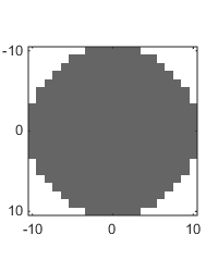
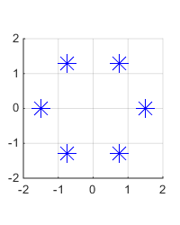
Figure 2. Wavefront data discretization ($21\times 21$) on telescope aperture in grey (left). Guide star asterism with 6 natural guide stars in a circle of 1.5 arcmin radius (right).

This mimics a Laser Tomography AO or a Multi-Object AO system and is well suited for evaluating the purely tomographic performance of the algorithms. The projection of the reconstructed layers onto the telescope aperture gives the optimal shape of the deformable mirror, thus, no sophisticated fitting step as, e.g., in Multi-Conjugate AO [15, 30, 22, 37], is needed between tomographic reconstruction and quality evaluation.

We consider two prominent atmospheric models: the 9-layer profile and the 40-layer profile, provided by the ESO. For comparison of the two profiles, the relative (logarithmic) densities in each Voronoi interval [4], i.e. the absolute weights $\rho_{l}$ divided by the interval length, are depicted in Figure 3. Additionally, the corresponding layer heights $h_{l}$ are marked, $l=1,\dots,L$ with $L=9$ and $L=40$ respectively.

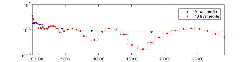
Figure 3. Height (in meter) vs. relative (log) density of atmospheric profiles: 9-layer (blue, triangle), 40-layer (red, circle).

We simulate a layered atmosphere following the von Karman model (6). By projection onto the telescope aperture in the center direction the simulated screen is obtained. The incoming wavefronts in guide star directions serve as input data for our reconstruction algorithms. After the reconstruction, the atmospheric layers are projected onto the telescope aperture in the center direction in order to get the shape of the deformable mirror.

Image quality is evaluated over the whole 3 arcmin field of view as well as in the center direction by means of the short-exposure Strehl ratio $S_{\varphi}$ [25], a value between 0 (worst) and 1 (best), which we approximate via the Marechal criterion (e.g. [32])

(27) $$S_{\varphi}\approx\exp\left(-\frac{1}{|\Omega_{D}|}\hskip 0.86108pt\|\overline{\varphi}-\varphi\|\hskip 0.86108pt^{2}_{L^{2}(\Omega_{D})}\right)\,,$$

with $\displaystyle\overline{\varphi}=\frac{1}{|\Omega_{D}|}\int_{\Omega_{D}}\varphi(r)\,dr\,$ the average phase over the aperture $\Omega_{D}$. Furthermore, we calculate the relative error in directions $\alpha_{g}$

(28) $$\varepsilon_{\alpha_{g}}=\frac{\hskip 0.86108pt\|{\bf A}_{\alpha_{g}}{\boldsymbol{\Phi}}^{\rm orig}\|\hskip 0.86108pt_{2}-\hskip 0.86108pt\|{\bf A}_{\alpha_{g}}{\boldsymbol{\Phi}}^{\rm rec}\|\hskip 0.86108pt_{2}}{\hskip 0.86108pt\|{\bf A}_{\alpha_{g}}{\boldsymbol{\Phi}}^{\rm orig}\|\hskip 0.86108pt_{2}}\,.$$

In the following, we only consider one time step, which spares us any concerns about temporal control and gain tuning. We refer to future work for a full simulation over more time steps.

5.2. Alternating minimization results

In Figure 4 we demonstrate the qualitative performance of the alternating minimization algorithm 1. We sample 512 realizations of the 9-layer atmospheric profile and compute the average radial Strehl ratio of our method and the standard gradient method [39, 31]. The alternating minimization algorithm outperforms the gradient method even if the latter is configured with exact layer weights.

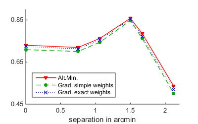
Figure 4. Alternating Minimization Algorithm 1 (red, triangle) vs. gradient method on fixed layer altitudes and exact weights (blue, cross) or simple weights ${\boldsymbol{\rho}}=(0.5,\frac{0.5}{8},\dots,\frac{0.5}{8})$ (green, circle): Radially averaged strehl ratio over 512 realizations of the 9-layer profile vs. separation from center direction (in arcmin).

The Strehl values are evaluated in 25 directions, i.e. in a $5\times 5$ square over the field of view. In Figure 4, the radial average is displayed over the separation in arc minutes from the center direction. At the guide star radius, Strehl ratios are largest, whereas due to the big field of view, the quality in the center is significantly lower. This is a typical behaviour for wide field of view AO: comparable results but for bigger telescope apertures were obtained, e.g. in [35].

Tests in Figure 4 have been performed with 100 (outer) iterations and 10 INNER iterations, a regularization parameter $\alpha=0.1$ and a ground-layer enforcing initial guess ${\boldsymbol{\rho}}_{\rm init}=(0.5,\frac{0.5}{8},\dots,\frac{0.5}{8})$. In the following, we stick to the choice of iteration number and starting value for the turbulence weights. A higher number of iterations improves quality by less than 1% of Strehl and relative error and does not influence the reconstructed turbulence weights significantly. Similarly, the choice of initial weights only slightly influences the performance of the algorithm. With uniform starting values, i.e. ${\boldsymbol{\rho}}_{\rm init}=(\frac{1}{9},\dots,\frac{1}{9})$, similar convergence behaviour but slightly lower quality was obtained. The large weight on the ground layer is physically motivated as most of the turbulence appears there.

In Figure 5 we depict results for Algorithm 1 with three clusters, i.e. $N=3$ (bottom), and without clustering, i.e. $N=1$ (top). The left column shows the reconstructed turbulence weights on the nine layers, along with the weights used for simulation. In the right column, the Strehl ratio (in center direction and averaged over the field of view) and the relative error for varying regularization parameters $\alpha$ are depicted. Please note, that the prescribed interval strength $d_{m}$ per cluster is displayed as line at value $d_{m}$ over all layers in cluster ${\mathcal{B}}_{m}$ in all following figures. The number and sizes of the clusters ${\mathcal{B}}_{m}$ and the corresponding weights $d_{m}$ can vary. Here, three clusters are modelled based on the idea of reducing the reconstruction effort to three instead of nine layers. Different choices of clusters and corresponding weights were tested yielding similar results.

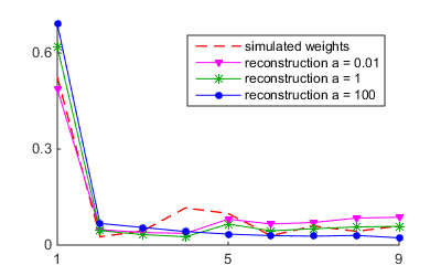
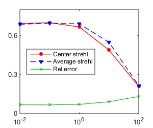
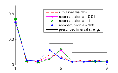
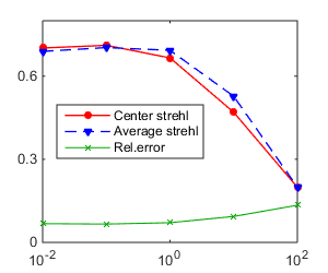
Figure 5. Alternating Minimization Algorithm 1: Turbulence weights vs. layers (left), Strehl and error vs. regularization parameter (right). 1 cluster (top), 3 clusters (bottom). 9-layer atmosphere, 100 (outer) iterations, INNER = 10.

We can observe that even for large regularization parameters $\alpha$ no sparse profile is obtained. This stems from the slow convergence in case of turbulence weights $\rho_{l}$ being close to zero. The direct solution of the optimality condition for ${\boldsymbol{\Phi}}$ in equation (21) would formally be identical to choosing INNER = $\infty$. The result for solving the optimality condition by direct matrix inversion with ${{\bf P}}^{-1}({\boldsymbol{\rho}})=\mbox{diag}\left(\frac{1}{\rho_{l}+\epsilon}\right)$ and $\epsilon\sim 10^{-10}$ for stabilization, is depicted in Figure 6. In this case, we can observe that the sparsity of the solution is more pronounced. A similar result as in Figure 6 can be obtained by considering the alternating minimization procedure for (12) by multiplying ${\bf P}({\boldsymbol{\rho}}_{i})$ to the update in the gradient step in Algorithm 1, as discussed at the end of Section 4.2.

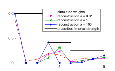
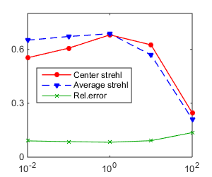
Figure 6. Alternating Minimization Algorithm 1 with direct solver for the optimality condition (21): Turbulence weights vs. layers (left), Strehl and error vs. regularization parameter (right). 9-layer atmosphere, 100 iterations, 3 clusters.

Therefore, we can conclude that the alternating minimization with the clustering approach approximates the true turbulence profile and with increasing regularization parameter also enforces sparsity. Moreover, the algorithm is easily integrated into existing reconstruction methods.

5.3. ISTA results

Compared to the alternative minimization approach, we can obtain a sparse turbulence profile with fewer iterations by utilizing the Iterative Shrinkage-Thresholding Algorithm (ISTA). Without the clustering, ISTA tends to recover all turbulence strength on the ground layer. As noted above, this is physically realistic. However, for wide field tomography problems higher vertical resolution is required. This can be guaranteed by introducing clusters.

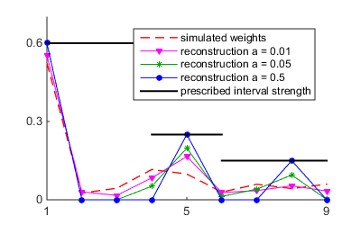
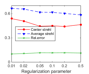
Figure 7. ISTA: Turbulence weights vs. layers (left), Strehl and error vs. regularization parameter (right). 9-layer atmosphere, 10 (outer) iterations, INNER = 10, 3 clusters.

In Figure 7 we demonstrate the results for ISTA with varying parameter $\alpha$. Recall that $\alpha$ influences the threshold for the shrinkage in Algorithm 2. The clustering approach approximates the true turbulence profile for small parameters $\alpha$ and with increasing $\alpha$ enforces sparsity, where only one layer per cluster has a nonzero turbulence weight.

For ISTA, 10 (outer) iterations along with 10 INNER iterations are already sufficient to reach a sparse turbulence profile and good quality. Compared to the alternating minimization algorithm, the quality is lower, in particular in the center. However, a sparse profile can be reached and the number of iterations is considerably lower.

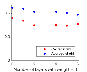
Figure 8. ISTA as in Figure 7: Strehl value vs. number of layers with zero weights.

In Figure 8 we can observe that the best reconstruction quality is obtained when all weights are non-zero. Naturally, the quality decreases when some weights are set to zero. However, reducing the number of non-zero turbulence weights, i.e., the number of reconstruction layers, e.g., from seven to three, does not alter the quality significantly. Thus, ISTA seems to be a promising approach to answering the question which layer altitudes are the most relevant for the reconstruction.

For the sake of convergence speed, the covariance matrix ${\bf C}_{\Psi}$ of the turbulence statistics can be omitted in the gradient step. With a proper choice of $\lambda$ and the number of ISTA iterations, both variants — with and without ${\bf C}_{\Psi}$ — yield very similar results and show comparable convergence behaviour.

The stepsize has to fulfill $\frac{1}{\lambda}\geq\frac{1}{\hskip 0.60275pt\|{\bf A}^{\ast}{\bf A}\|\hskip 0.60275pt}=\frac{1}{\lambda_{max}({\bf A}^{\ast}{\bf A})}\approx 0.022$. In the examples presented here, we chose a fix stepsize of 0.25, i.e. $\lambda=4$, which leads to fast convergence. A more sophisticated stepsize choice, such as the classical steepest descent stepsize can improve quality, in particular, the center Strehl ratio by several percent and the average Strehl ratio by a few percent.

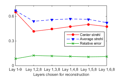
Figure 9. ISTA chooses the best reconstruction layer altitudes: Strehl and error vs. reconstruction layers. Gradient method on fixed layer altitudes and heights, 100 iterations, reconstruction on all 9 layers (leftmost) and on 3 layers (cluster 1 and 3 fixed, i.e. layers 1 and 8, and varying layer in cluster 2).

In Figure 9 we demonstrate that ISTA recovers the qualitatively optimal reconstruction layer altitude per cluster. We run ISTA as in Figure 7 with $\alpha=0.5$, and determine the preselected candidates for non-zero reconstruction layers, i.e., layers 1, 5 and 8. Then we apply a standard gradient method [39, 31] with a fixed number of layers and altitudes and heights set to different combinations. We fix layer 1 and 8 and vary the reconstruction layers in cluster 2 (layers 2 to 6). One can observe, that the reconstruction layer 5 — chosen as optimal both by ISTA and the alternating minimization for cluster 2 — yields the best results compared to a reconstruction with layers 2, 3, 4, and 6 instead. This clearly demonstrates the potential of our algorithms to automatically select the “best” model (layers).

Furthermore, Figure 10 shows that the choice of reconstruction layer 5 by ISTA and the alternating minimization for cluster 2 is consistent with the variation of cluster sizes.

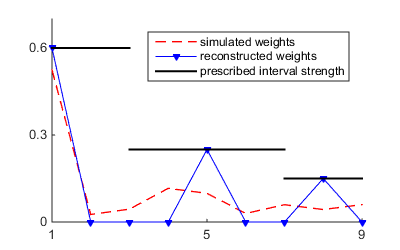
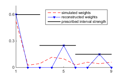
Figure 10. Block variation for ISTA (settings as in Figure 7): Turbulence weights vs. layers.

Similar results can be obtained for the 40-layer atmosphere. In Figure 11, we can observe, that already 50 (outer) iterations suffice to guarantee convergence to one layer per cluster. For $\alpha$ large enough, i.e., greater than 0.05, the convergence to the non-zero layers 1, 2, 12, 24 and 37, is robust with respect to varying cluster sizes and weights. As for the 9-layer atmosphere, the quality is very stable over the number of iterations.

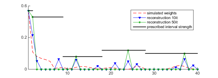
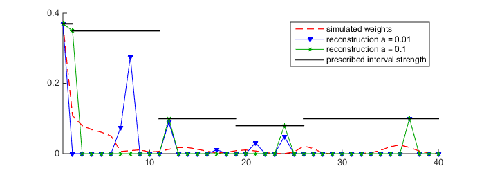
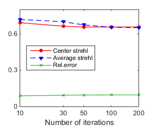
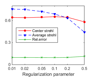
Figure 11. ISTA on 40-layer atmosphere: Turbulence weights vs. layers (top), Strehl and error vs. number of (outer) iterations (bottom, left), vs. regularization parameter (bottom, right). INNER = 10, 5 clusters.

Using the FISTA-variant of Algorithm 3, a speed up in convergence can be obtained. However, in these examples, the reduction in the computational effort is rather small, as only few iterations are needed anyway. However, this speed up could be a crucial point for systems with finer resolution such as the ELT.

The computational cost of one gradient step is determined by the operators ${\bf A},{\bf A}^{\ast}$ and the application of ${\bf C}_{\Psi}^{-1}$. The numerical effort of ${\bf A}$ and ${\bf A}^{\ast}$ mainly stems from bilinear interpolation. The application of the inverse covariance matrix ${\bf C}_{\Psi}^{-1}$ is the most costly step in both Algorithms 1 and 3. Note, that in Algorithm 1, this has to be performed in each INNER step, i.e., $k\cdot i$ times, while in ISTA, it is only needed in the shrinkage step, i.e., $i$ times. By thresholding, the dense matrices $C_{\Phi}^{-1}$ can be sparsified without loss of qualitative performance. However, more sophisticated methods, as, e.g., in [42, 43], are needed to efficiently apply the method for larger systems with finer resolution. Both algorithms can be parallelized on the reconstruction layers, as well as in the guide star directions.

	$L$	cost per it	$L$	cost per it
original atmosphere	40	$3908n$	9	$839n$
downsampled atmosphere	5	$443n$	3	$245n$
speed up factor	8.8		3.4

Table 1. Upper bounds of the computational cost estimates per standard gradient iteration, one iteration costs $(16G+3)nL+(2-9G)n$, $G=6$ guide stars and $L$ the number of reconstruction layers.

Table 1 shows the computational cost estimates and speed up factors for a standard gradient iteration [39] (with fixed turbulence heights and weights). With the resulting downsampled turbulence profiles from the alternating minimization algorithm or ISTA, we could reach speed up factors of 8.8 and 3.4 for the 40-layer and 9-layer atmosphere, respectively. Again, this should serve as a justification of the proposed methods as a tool for joint identification and model reduction.

6. Conclusion

In this paper, we presented a new reconstruction algorithm for atmospheric tomography that includes an automatic model optimization of the reconstruction profile. We derived the corresponding Bayesian model and presented two different algorithms to solve the joint optimization with respect to the atmospheric layers and their turbulence weights. Our numerical results suggest that both algorithms choose optimal reconstruction heights which leads to a significant speed up while still results of good quality are obtained. Moreover, our algorithms can be easily adapted for a two-step method, such as [22], with wavefront sensor measurements as input data instead of incoming wavefronts.

We believe that our method is very promising especially for wide field of view AO systems as the approach unites the idea of conventional compression algorithms for a layered atmosphere and the tomographic reconstruction itself. The numerical experiments presented here indicate that the methods are not yet feasible for real-time usage in present-day AO systems with many degrees of freedom due to some rather time-consuming steps like the application of the turbulence statistics. However, our model reduction approach can still be used offline for profile optimization, running in parallel to a standard real-time reconstructor. The updated and optimized profile can then be included into the reconstructor whenever available. This allows to adapt on the fly to changing atmospheric conditions.

References

- [1] M. Abramowitz and I. A. Stegun. Handbook of mathematical functions with formulas, graphs, and mathematical tables, volume 55 of National Bureau of Standards Applied Mathematics Series. 1964.
- [2] G. Aubert and P. Kornprobst. Mathematical problems in image processing, volume 147 of Applied Mathematical Sciences. Springer, New York, second edition, 2006.
- [3] G. Auzinger. New Reconstruction Approaches in Adaptive Optics for Extremely Large Telescopes. PhD thesis, Johannes Kepler University Linz, 2015.
- [4] G. Auzinger. On choosing layer profiles in atmospheric tomography. Journal of Physics: Conference Series (JPCS), 595(012001), 2015. URL: http://dx.doi.org/10.1088/1742-6596/595/1/012001.
- [5] A. Beck and M. Teboulle. A fast iterative shrinkage-thresholding algorithm for linear inverse problems. SIAM journal on imaging sciences, 2(1):183–202, 2009.
- [6] A. Beghi, A. Cenedese, and A. Masiero. Stochastic realization approach to the efficient simulation of phase screens. JOSA A, 25(2):515–525, 2008.
- [7] D. Bertsekas. Nonlinear Programming. Athena Scientific, Belmont, MA, 1999.
- [8] C. S. Boyd, N. Parikh, E. Chu, B. Peleato, J. Eckstein, S. Boyd, N. Parikh, E. Chu, B. Peleato, and J. Eckstein. Distributed optimization and statistical learning via the alternating direction method of multipliers, 2010.
- [9] A. Chambolle and P.-L. Lions. Image recovery via total variation minimization and related problems. Numer. Math., 76(2):167–188, 1997.
- [10] A. Cortés, B. Neichel, A. Guesalaga, J. Osborn, F. Rigaut, and D. Guzman. Atmospheric turbulence profiling using multiple laser star wavefront sensors. Monthly Notices of the Royal Astronomical Society, 427(3):2089–2099, 2012.
- [11] A. Costille and T. Fusco. Impact of cn2 profile on tomographic reconstruction performance: application to e-elt wide field ao systems. In SPIE Astronomical Telescopes+ Instrumentation, pages 844757–844757. International Society for Optics and Photonics, 2012.
- [12] A. Costille and T. Fusco. Impact of cn2 profile on tomographic reconstruction performance: application to e-elt wide field ao systems. volume 8447, pages 844757–844757–9, 2012.
- [13] P. Druilhet, J.-M. Marin, et al. Invariant HPD credible sets and MAP estimators. Bayesian Analysis, 2(4):681–691, 2007.
- [14] M. Eslitzbichler, C. Pechstein, and R. Ramlau. An h1-kaczmarz reconstructor for atmospheric tomography. Journal of Inverse and Ill-Posed Problems, 21(3):431–450, 2013.
- [15] T. Fusco, J.-M. Conan, G. Rousset, L. Mugnier, and V. Michau. Optimal wave-front reconstruction strategies for multi conjugate adaptive optics. J. Opt. Soc. Am. A, 18(10):2527–2538, 2001.
- [16] T. Fusco and A. Costille. Impact of cn2 profile structure on wide-field ao performance. In SPIE Astronomical Telescopes+ Instrumentation, pages 77360J–77360J. International Society for Optics and Photonics, 2010.
- [17] I. M. Gel′fand and N. Y. Vilenkin. Generalized functions. Vol. 4. Academic Press [Harcourt Brace Jovanovich, Publishers], New York-London, 1964 [1977]. Applications of harmonic analysis, Translated from the Russian by Amiel Feinstein.
- [18] E. Gendron, C. Morel, J. Osborn, O. Martin, D. Gratadour, F. Vidal, M. Le Louarn, and G. Rousset. Robustness of tomographic reconstructors versus real atmospheric profiles in the elt perspective. volume 9148, pages 91484N–91484N–13, 2014.
- [19] L. Gilles and B. Ellerbroek. Real-time turbulence profiling with a pair of laser guide star shack–hartmann wavefront sensors for wide-field adaptive optics systems on large to extremely large telescopes. JOSA A, 27(11):A76–A83, 2010.
- [20] T. Goldstein and S. Osher. The split Bregman method for -regularized problems. SIAM J. Imaging Sci., 2(2):323–343, 2009.
- [21] T. Helin and M. Burger. Maximum a posteriori probability estimates in infinite-dimensional bayesian inverse problems. Inverse Problems, 31(8):085009, 2015.
- [22] T. Helin and M. Yudytskiy. Wavelet methods in multi-conjugate adaptive optics. Inverse Problems, 29(8):085003, 2013.
- [23] M. R. Hestenes. Multiplier and gradient methods. J. Optimization Theory Appl., 4:303–320, 1969.
- [24] A. N. Kolmogorov. The local structure of turbulence in incompressible viscous fluid for very large reynolds numbers. In Dokl. Akad. Nauk SSSR, volume 30, pages 299–303, 1941.
- [25] M. Le Louarn, C. Verinaud, and V. Korkiakoski. Simulation of mcao on (extremely) large telescopes. Comptes Rendus Physique, 6(10):1070–1080, 2005.
- [26] E. Masciadri, G. Lombardi, and F. Lascaux. On the comparison between mass and generalized-scidar techniques. Monthly Notices of the Royal Astronomical Society, 2014.
- [27] S. Osher, M. Burger, D. Goldfarb, J. Xu, and W. Yin. An iterative regularization method for total variation-based image restoration. Multiscale Model. Simul., 4(2):460–489 (electronic), 2005.
- [28] M. J. D. Powell. A method for nonlinear constraints in minimization problems. In Optimization (Sympos., Univ. Keele, Keele, 1968), pages 283–298. Academic Press, London, 1969.
- [29] M. J. D. Powell. On search directions for minimization algorithms. Math. Programming, 4:193–201, 1973.
- [30] R. Ramlau and M. Rosensteiner. An efficient solution to the atmospheric turbulence tomography problem using Kaczmarz iteration. Inverse Problems, 28(9):095004, 2012.
- [31] R. Ramlau, D. Saxenhuber, and M. Yudytskiy. Iterative reconstruction methods in atmospheric tomography: FEWHA, Kaczmarz and Gradient-based algorithm. In Proc. SPIE, volume 9148, pages 91480Q–91480Q–15, 2014.
- [32] F. Roddier. Adaptive Optics in Astronomy. Cambridge, U.K. ; New York : Cambridge University Press, Cambridge, 1999.
- [33] P. Rodríguez and B. Wohlberg. An iteratively reweighted norm algorithm for minimization of total variation functionals. IEEE Signal Processing Letters, 14:948–951, 2007.
- [34] M. C. Roggemann and B. Welsh. Imaging through turbulence. CRC Press laser and optical science and technology series. CRC Press, 1996.
- [35] M. Rosensteiner and R. Ramlau. The Kaczmarz algorithm for multi-conjugate adaptive optics with laser guide stars. J. Opt. Soc. Am. A, 30(8):1680–1686, 2013.
- [36] G. Rousset et al. EAGLE MOAO system conceptual design and related technologies. Society of Photo-Optical Instrumentation Engineers (SPIE) Conference Series, 7736, 2010.
- [37] M. Y. S. Raffetseder, R. Ramlau. Optimal mirror deformation for multi conjugate adaptive optics systems. submitted, 2015.
- [38] M. Sarazin, M. Le Louarn, J. Ascenso, G. Lombardi, and J. Navarrete. Defining reference turbulence profiles for e-elt ao performance simulations. In Third AO4ELT Conference Adaptive Optics for ELTs Proc., Edited by S. Esposito and L. Fini, 2013.
- [39] D. Saxenhuber and R. Ramlau. A gradient-based method for atmospheric tomography. submitted, 2015.
- [40] J. Vernin, C. Muñoz Tuñón, M. Sarazin, H. V. Ramió, A. M. Varela, H. Trinquet, J. M. Delgado, J. J. Fuensalida, M. Reyes, A. Benhida, Z. Benkhaldoun, D. G. Lambas, Y. Hach, M. Lazrek, G. Lombardi, J. Navarrete, P. Recabarren, V. Renzi, M. Sabil, and R. Vrech. European extremely large telescope site characterization i: Overview. Publications of the Astronomical Society of the Pacific, 123(909):pp. 1334–1346, 2011.
- [41] T. von Karman. Mechanische Ähnlichkeit und Turbulenz. 3rd International Congress of Applied Mechanics, 1930.
- [42] M. Yudytskiy, T. Helin, and R. Ramlau. A frequency dependent preconditioned wavelet method for atmospheric tomography. In Third AO4ELT Conference - Adaptive Optics for Extremely Large Telescopes, May 2013.
- [43] M. Yudytskiy, T. Helin, and R. Ramlau. Finite element-wavelet hybrid algorithm for atmospheric tomography. J. Opt. Soc. Am. A, 31(3):550–560, Mar 2014.
- [44] M. Zhu and T. Chan. An efficient primal-dual hybrid gradient algorithm for total variatoin image restoration. Technical Report CAM Report 08-34, UCLA, Los Angeles, 2008.