An introduction to the analysis and implementation of sparse grid finite element methods

Abstract

Our goal is to present an elementary approach to the analysis and programming of sparse grid finite element methods. This family of schemes can compute accurate solutions to partial differential equations, but using far fewer degrees of freedom than their classical counterparts. After a brief discussion of the classical Galerkin finite element method with bilinear elements, we give a short analysis of what is probably the simplest sparse grid method: the two-scale technique of Lin et al. LiYa01 . We then demonstrate how to extend this to a multiscale sparse grid method which, up to choice of basis, is equivalent to the hierarchical approach, as described in, e.g., BuGr04 . However, by presenting it as an extension of the two-scale method, we can give an elementary treatment of its analysis and implementation. For each method considered, we provide MATLAB code, and a comparison of accuracy and computational costs.

1 Introduction

Sparse grid methods provide a means of approximating functions and data in a way that avoids the notorious “curse of dimensionality”: for fixed accuracy, the computational effort required by classical methods grows exponentially in the number of dimensions. Sparse grid methods hold out the hope of retaining the accuracy of classical techniques, but at a cost that is essentially independent of the number of dimensions.

An important application of sparse grid methods is the solution of partial differential equations (PDEs) by finite element methods (FEMs). Naturally, the solution to a PDE is found in an infinite dimensional space. A FEM first reformulates the problem as an integral equation, and then restricts this problem to a suitable finite-dimensional subspace; most typically, this subspace is comprised of piecewise polynomials. This “restricted” problem can be expressed as a matrix-vector equation; solving it gives the finite element approximation to the solution of the PDE. For many FEMs, including those considered in this article, this solution is the best possible approximation (with respect to a certain norm) that one can find in the finite-dimensional subspace. That is, the accuracy of the FEM solution depends on the approximation properties of the finite dimensional space.

The main computational cost incurred by a FEM is in the solution of the matrix-vector equation. This linear system is sparse, and amenable to solution by direct methods, such as Cholesky-factorisation, if it is not too large, or by highly efficient iterative methods, such as multigrid methods, for larger systems. The order of the system matrix is the dimension of the finite-element space, and so great computational efficiencies can be gained over classical FEMs by constructing a finite-dimensional space of reduced size without compromising the approximation properties: this is what is achieved by sparse grid methods.

We will consider the numerical solution of the following PDE

$$Lu:=-\Delta u+ru=f(x,y)\quad\text{in }\Omega:=(0,1)^{2},$$ (1.1a)

$$u=0\quad\text{on }\partial\Omega.$$ (1.1b)

Here $r$ is a positive constant and so, for simplicity, we shall take $r=1$, but $f$ is an arbitrary function. Our choice of problem is motivated by the desire, for the purposes of exposition, to keep the setting as simple as possible, but without trivialising it. The main advantages of choosing $r$ to be constant are that no quadrature is required when computing the system matrix, and that accurate solutions can be obtained using a uniform mesh. Thus, the construction of the system matrix for the standard Galerkin FEM is reduced to several lines of code, which we show how to do in Section 2. In Section 3 we show how to develop the two-scale sparse grid method and, in Section 4 show how to extend this to a multiscale setting. A comparison of the accuracy and efficiency of the methods is given in Section 5. We stress that the choice of constant $r$ in (1.1) is only to simplify the implementation of the standard Galerkin method: our implementation of the sparse grid methods is identical for variable $r$, and would require only minor modifications for nonuniform tensor product meshes.

We aim to provide an introduction to the mathematical analysis and computer implementation of sparse grids that is accessible to readers who have a basic knowledge of finite element methods. For someone who is new to FEMs, we propose (SuMa03, , Chapter 14) as a primer for the key concepts. An extensive mathematical treatment is given in BrSc08 : we use results from its early chapters.

We do not aim to present a comprehensive overview of the state of the art sparse grid methods: there are many important contributions to this area which we do not cite. However, we hope that, having read this article, and experimented with the MATLAB programs provided, the reader will be motivated to learn more from important references in the area, such as BuGr04 .

1.1 MATLAB code

All our numerical examples are implemented in MATLAB. Full source code is available from www.maths.nuigalway.ie/$\sim$niall/SparseGrids while snippets are presented in the text. Details of individual functions are given in the relevant sections. For those using MATLAB for the first time, we recommend Dris09 as a readable introduction. Many of the finer points of programming in MATLAB are presented in Mole04 and HiHi05 . A detailed study of programming FEMs in MATLAB may be found in Gock06 .

We make use of the freely-available Chebfun toolbox DrHa14 to allow the user to choose their own test problem, for which the corresponding $f$ is automatically computed. We also use Chebfun for some computations related to calculating the error. (We highly recommend using Chebfun Version 5 or later, as some of the operations we use are significantly faster than in earlier versions). Only Test_FEM.m, the main test harness, uses Chebfun. That script contains comments to show how it may be modified to avoid using Chebfun, and thus run on Octave octave:2014 . We have found the direct linear solver (“backslash”) to be less efficient in Octave than MATLAB, and thus timing may be qualitatively different from those presented here (though no doubt some optimisations are possible).

1.2 Notation

We use the standard $L_{2}$ inner product and norm:

$$(u,v):=\int_{\Omega}uv\,d\Omega,\qquad\|u\|_{0,\Omega}=\sqrt{(u,u)}.$$

The bilinear form, $B(\cdot,\cdot)$ associated with (1.1) is

$$B(u,v)=(\nabla u,\nabla v)+(ru,v),$$

which induces the energy norm

$$\|u\|_{B}=\{\|\nabla u\|_{0,\Omega}^{2}+\|u\|_{0,\Omega}^{2}\}^{1/2}.$$ (1.2)

The space of functions whose (weak) $k^{\mathrm{th}}$ derivatives are integrable on a domain $\omega$ is denoted by $H^{k}(\omega)$, and if these functions also vanish on the boundary of $\omega$ it is $H^{k}_{0}(\omega)$. See, e.g., (BrSc08, , Chap. 2) for more formal definitions.

Throughout this paper the letter $C$, with or without subscript, denotes a generic positive constant that is independent of the discretization parameter, $N$, and the scale of the method $k$, and may stand for different values in different places, even within a single equation or inequality.

2 Standard Galerkin finite element method

2.1 A Galerkin FEM with bilinear elements

The weak form of (1.1) with $r=1$ is: find u $\in H^{1}_{0}(\Omega)$ such that

$$B(u,v):=(\nabla u,\nabla v)+(u,v)=(f,v)\quad\forall v\in H^{1}_{0}(\Omega).$$ (2.1)

A Galerkin FEM is obtained by replacing $H_{0}^{1}(\Omega)$ in (2.1) with a suitable finite-dimensional subspace. We will take this to be the space of piecewise bilinear functions on a uniform mesh with $N_{x}$ equally sized intervals in one coordinate direction and $N_{y}$ equally sized intervals in the other. We first form a one-dimensional mesh $\omega_{x}=\{x_{0},x_{1},\dots,x_{N_{x}}\}$, where $x_{i}=i/N_{x}$. Any piecewise linear function on this mesh can be uniquely expressed in terms of the so-called “hat” functions

$$\psi^{N}_{i}(x)=\begin{cases}\displaystyle\frac{x-x_{i-1}}{x_{i}-x_{i-1}}&\text{if }x_{i-1}\leq x<x_{i},\\ \displaystyle\frac{x_{i+1}-x}{x_{i+1}-x_{i}}&\text{if }x_{i}\leq x<x_{i+1},\\ 0&\text{otherwise.}\end{cases}$$ (2.2)

Similarly, we can construct a mesh in the $y$-direction: $\omega_{y}=\{y_{0},y_{1},\dots,y_{N_{y}}\}$, where $y_{j}=j/N_{y}$. We can form a two-dimensional $N_{x}\times N_{y}$ mesh by taking the Cartesian product of $\omega_{x}$ and $\omega_{y}$, and then define the space of piecewise bilinear functions, $V_{N_{x},N_{y}}\subset H^{1}_{0}(\Omega)$ as

$$V_{N_{x},N_{y}}=\text{span}\left\{\psi^{N_{x}}_{i}(x)\psi^{N_{y}}_{j}(y)\right\}^{i=1:N_{x}-1}_{j=1:N_{y}-1},$$ (2.3)

where here we have adopted the compact MATLAB notation $i=1\!:\!N_{x}-1$ meaning $i=1,2,\dots,N_{x}-1$. (Later we use expressions such as $i=1\!:\!2\!:\!N_{x}-1$ meaning $i=1,3,5,\dots,N_{x}-1$).

For sparse grid methods, we will be interested in meshes where $N_{x}\neq N_{y}$. However, for the classical Galerkin method, we take $N_{x}=N_{y}=N$. Thus, our finite element method for (1.1) is: find $u_{N,N}\in{V}_{N,N}$ such that

$$B(u_{N,N},v_{N,N})=(f,v_{N,N})\quad\text{ for all }v_{N,N}\in{V}_{N,N}.$$ (2.4)

2.2 Analysis of the Galerkin FEM

The bilinear form defined in (2.1) is continuous and coercive, so (2.4) possesses a unique solution. Moreover, as noted in (LMSZ09, , Section 3), one has the quasi-optimal bound:

$$\|u-u_{N,N}\|_{B}\leq C\inf_{\psi\in V_{N,N}(\Omega)}\|u-\psi\|_{B}.$$

To complete the analysis, we can choose a good approximation of $u$ in $V_{N,N}$. A natural choice is the nodal interpolant of $u$. To be precise, let $I_{N,N}:C(\bar{\Omega})\rightarrow V_{N,N}$ be the nodal piecewise bilinear interpolation operator that projects onto $V_{N,N}$. Since $I_{N,N}u\in V_{N,N}$, one can complete the error analysis using the following classical results. For a derivation, see, e.g., GGRS07 .

Lemma 1

Let $\tau$ be any mesh rectangle of size $h\times h$. Let $u\in H^{2}(\tau)$. Then its piecewise bilinear nodal interpolant, $I_{N,N}u$, satisfies the bounds

$$\|u-I_{N,N}u\|_{0,\Omega}\leq Ch^{2}(\|u_{xx}\|_{0,\Omega}+\|u_{xy}\|_{0,\Omega}+\|u_{yy}\|_{0,\Omega}),$$ (2.5a)

$$\|(u-I_{N,N}u)_{x}\|_{0,\Omega}\leq Ch(\|u_{xx}\|_{0,\Omega}+\|u_{xy}\|_{0,\Omega}),$$ (2.5b)

$$\|(u-I_{N,N}u)_{y}\|_{0,\Omega}\leq Ch(\|u_{xy}\|_{0,\Omega}+\|u_{yy}\|_{0,\Omega}).$$ (2.5c)

The following results follow directly from Lemma 1.

Lemma 2

Suppose $\Omega$= $(0,1)^{2}$. Let $u\in H^{2}_{0}(\Omega)$ and $I_{N,N}u$ be its piecewise bilinear nodal interpolant. Then there exists a constant $C$, independent of $N$, such that

$$\|u-I_{N,N}u\|_{0,\Omega}\leq CN^{-2},\quad\text{ and }\quad\|\nabla(u-I_{N,N}u)\|_{0,\Omega}\leq CN^{-1}.$$

Consequently, $\|u-I_{N,N}u\|_{B}\leq CN^{-1}$.

It follows immediately from these results that there exists a constant $C$, independent of $N$, such that

$$\|u-u_{N,N}\|_{B}\leq CN^{-1}.$$ (2.6)

2.3 Implementation of the Galerkin FEM

To implement the method (2.4), we need to construct and solve a linear system of equations. A useful FEM program also requires ancillary tools, for example, to visualise the solution and to estimate errors.

Because the test problem we have chosen has a constant left-hand side, the system matrix can be constructed in a few lines, and without resorting to numerical quadrature. Also, because elements of the space defined in (2.3) are expressed as products of one-dimensional functions, the system matrix can be expressed in terms of (Kronecker) products of matrices arising from discretizing one-dimensional problems. We now explain how this can be done. We begin with the one-dimensional analogue of (1.1):

$$-u^{\prime\prime}(x)+u(x)=f(x)\text{ on }(0,1),\quad\text{ with }\quad u(0)=u(1)=1.$$

Its finite element formulation is: find $u_{N}\in{V}_{N}(0,1)$ such that

$$(u_{N}^{\prime},v^{\prime}_{N})+(u_{N},v_{N})=(f,v_{N})\quad\text{ for all }v_{N}\in{V}_{N}(0,1).$$ (2.7)

This $u_{N}$ can be expressed as a linear combination of the $\psi^{N}_{i}$ defined in (2.2):

$$u_{N}=\sum_{j=1,\dots,N-1}\mu_{j}\psi^{N}_{j}(x).$$

Here the $\mu_{j}$ are the $N-1$ unknowns determined by solving the $N-1$ equations obtained by taking $v_{N}=\psi_{i}^{N}(x)$, for $i=1,\dots,N-1$, in (2.7). Say we write the system matrix for these equations as $(a_{2}+a_{0})$, where $a_{2}$ (usually called the stiffness matrix) and $a_{0}$ (the mass matrix) are $(N-1)\times(N-1)$ matrices that correspond, respectively, to the terms $(u_{N}^{\prime},v^{\prime}_{N})$ and $(u_{N},v_{N})$. Then $a_{2}$ and $a_{0}$ are tridiagonal matrices whose stencils are, respectively,

$$N\begin{pmatrix}-1&2&-1\end{pmatrix}\quad\text{ and }\quad\frac{1}{6N}\begin{pmatrix}1&4&1\end{pmatrix}.$$

For the two-dimensional problem (1.1) there are $(N-1)^{2}$ unknowns to be determined. Each of these are associated with a node on the mesh, which we must number uniquely. We will follow a standard convention, and use lexicographic ordering. That is, the node at $(x_{i},y_{j})$ is labelled $k=i+(N-1)(j-1)$. The basis function associated with this node is $\phi_{k}^{N}=\psi_{i}^{N}(x)\psi_{j}^{N}(x)$. Then the $(N-1)^{2}$ equations in the linear system for (2.4) can be written as

$$B(u_{N,N},\phi_{k}^{N})=(f,\phi_{k}^{N}),\quad\text{ for }\quad k=1,\dots(N-1)^{2}.$$

Since $r=1$, this can be expressed in terms of Kronecker products (see, e.g., (Laub05, , Chap. 13)) of the one-dimensional matrices described above:

$$A=a_{0}\otimes a_{2}+a_{2}\otimes a_{0}+a_{0}\otimes a_{0}.$$ (2.8)

The MATLAB code for constructing this matrix is found in FEM_System_Matrix.m. The main computational cost of executing that function is incurred by computing the Kronecker products. Therefore, to improve efficiency, (2.8) is coded as

⬇

A = kron(a0,a2) + kron(a2+a0,a0);

The right-hand side of the finite element linear system is computed by the function FEM_RHS.m. As is well understood, the order of accuracy of this quadrature must be at least that of the underlying scheme, in order for quadrature errors not to pollute the FEM solution. As given, the code uses a two-point Gaussian quadrature rule (in each direction) to compute

$$b_{k}=(f,\phi_{k}^{N}),\quad\text{ for }\quad k=1,\dots,(N-1)^{2}.$$ (2.9)

It can be easily adapted to use a different quadrature scheme (see, e.g., (GGRS07, , §4.5) for higher order Gauss-Legendre and Gauss-Lobatto rules for these elements).

To compute the error, we need to calculate $\sqrt{B(u-u_{N,N},u-u_{N,N})}$. Using Galerkin orthogonality, since $u$ solves (2.1) and $u_{N,N}$ solves (2.4), one sees that

$$B(u-u_{N,N},u-u_{N,N})=(f,u)-(f,u_{N,N}).$$ (2.10)

The first term on the right-hand side can be computed (up to machine precision) using Chebfun

⬇

Energy = integral2(u.*f,[0, 1, 0, 1]);

where $u$ and $f$ are chebfuns that represent the solution and right-hand side in (1.1). We estimate the term $(f,u_{N,N})$ as

⬇

Galerkin_Energy = uN’*b;

where uN is the solution vector, and ${b}$ is the right-hand side of the linear system, as defined in (2.9).

2.4 Numerical results for the Galerkin FEM

The test harness for the code described in Section 2.3 is named Test_FEM.m. As given, it implements the method for $N=2^{4},2^{5},\dots,2^{10}$, so the problem size does not exceed what may be solved on a standard desktop computer. Indeed, on a computer with at least 8Gb of RAM, it should run with $N=2^{11}$ intervals in each coordinate direction, resolving a total of $4,190,209$ degrees of freedom. We present the results in Figure 1, which were generated on a computer equipped with 32Gb of RAM, allowing to solve problems with $N=2^{12}$ intervals in each direction (i.e., $16,769,025$ degrees of freedom). One can observe that the method is first-order convergent, which is in agreement with (2.6). 1(b) shows $u-u_{N,N}$ for $N=64$.

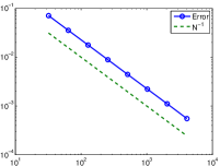
(a) Rate of convergence

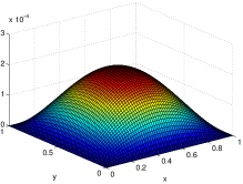
(b) $u-u_{64,64}$

Figure 1: Left: convergence of the classical Galerkin method. Right: the error in the Galerkin solutions with $N=64$

3 A two-scale sparse grid finite element method

The main purpose of this article is to introduce sparse grid FEMs, which can achieve accuracy that is comparable to the classical Galerkin FEM of Section 2, but with much fewer degrees of freedom. As we describe in Section 4, most of these methods are described as multiscale or “multi-level”. However, the simplest sparse grid method is, arguably, the two-scale method proposed by Lin et al. LiYa01 . Those authors were motivated to study the method in order to prove certain superconvergence results. For us, its appeal is the simplicity of its implementation and analysis. By extending our MATLAB program from Section 2.3 by only a few lines of code, we can obtain a solution that has, essentially, the same accuracy as the classical FEM, but using $N^{4/3}$ rather than $N^{2}$ degrees of freedom. Moreover, having established some basic principles of the method in this simple setting, we are well equipped to consider the more complicated multiscale method of Section 4.

Recalling Section 2.2, the error analysis of a FEM follows directly from establishing the approximation properties of the finite dimensional space and, typically, this follows from an analysis of a particular candidate for an approximation of the true solution: the nodal interpolant. Therefore, in Section 3.1 we describe a two-scale interpolation operator. This naturally leads to a two-scale FEM, the implementation of which is described in Section 3.3. That section also contains numerical results that allow us to verify that the accuracy of the solution is very similar to the FEM of Section 2. Although the whole motivation of the method is to reduce the computational cost of implementing a classical Galerkin method, we postpone a discussion of the efficiency of the method to Section 5, where we compare the classical, two-scale and multiscale methods directly.

We will make repeated use of the following one-dimensional interpolation bounds. Their proofs can be found in (SuMa03, , Theorem. 14.7).

Theorem 3.1

Suppose that $u\in H^{2}(0,1)\cap H^{1}_{0}(0,1)$. Then the piecewise linear interpolant $I_{N}u$ satisfies

$$\|u-I_{N}u\|_{0,\Omega}\leq Ch_{i}^{2}\|u^{\prime\prime}\|_{0,\Omega},\quad\text{ and }\quad\|u^{\prime}-(I_{N}u)^{\prime}\|_{0,\Omega}\leq Ch_{i}\|u^{\prime\prime}\|_{0,\Omega},$$ (3.1)

for $i=1,2,...,N$, and $h_{i}=x_{i}-x_{i-1}$.

3.1 The two-scale interpolant

Let $V_{N_{x}}([0,1])$ be the space of piecewise linear functions defined on the one-dimensional mesh with $N_{x}$ intervals on $[0,1]$. Define $V_{N_{y}}([0,1])$ in the same way. Then let $V_{N_{x},N_{y}}$ be the tensor product space $V_{N_{x}}([0,1])\times V_{N_{y}}([0,1])$. Let $I_{N_{x},N_{y}}:C(\bar{\Omega})\rightarrow V_{N_{x},N_{y}}$ be the nodal piecewise bilinear interpolation operator that projects onto $V_{N_{x},N_{y}}$. Write $I_{N_{x},0}$ for the interpolation operator that interpolates only in the $x$-direction, so $I_{N_{x},0}:C(\bar{\Omega})\rightarrow V_{N_{x}}([0,1])\times C([0,1])$. Similarly, let $I_{0,N_{y}}:C(\bar{\Omega})\rightarrow C([0,1])\times V_{N_{y}}([0,1])$ interpolate only in the $y$-direction. Then clearly

$$I_{N_{x},N_{y}}=I_{N_{x},0}\circ I_{0,N_{y}}=I_{0,N_{y}}\circ I_{N_{x},0},$$ (3.2a)

$$\frac{\partial}{\partial x}I_{N_{x},N_{y}}=I_{0,N_{y}}\circ\frac{\partial}{\partial x}I_{N_{x},0},$$ (3.2b)

$$\frac{\partial}{\partial y}I_{N_{x},N_{y}}=I_{N_{x},0}\circ\frac{\partial}{\partial y}I_{0,N_{y}}.$$ (3.2c)

In this section we present an interpretation of the two-scale technique outlined in LMSZ09 . The two-scale interpolation operator $\widehat{I}_{N,N}:C(\bar{\Omega})\rightarrow V_{N,N}$ is defined as

$$\widehat{I}_{N,N}u=I_{N,\sigma(N)}+I_{\sigma(N),N}-I_{\sigma(N),\sigma(N)},$$ (3.3)

where $\sigma(N)$ is an integer that divides $N$. The following identity appears in LMSZ09 , and is an integral component of the following two-scale interpolation analysis:

$$I_{N,N}u-\widehat{I}_{N,N}u=(I_{N,0}-I_{\sigma(N),0})(I_{0,N}-I_{0,\sigma(N)}).$$ (3.4)

Theorem 3.2

Suppose $\Omega=(0,1)^{2}$ and $u\in H^{1}_{0}(0,1)$. Let $I_{N,N}u$ be the bilinear interpolant of $u$ on $\Omega_{N,N}$, and $\widehat{I}_{N,N}u$ be the two-scale bilinear interpolant of $u$ described in (3.3). Then there exists a constant $C$ independent of $N$, such that

$$\|\widehat{I}_{N,N}u-I_{N,N}u\|_{B}\leq C\sigma(N)^{-3}.$$

Proof

First from (3.4), and then by the first inequality in (3.1), one has

$$\|\widehat{I}_{N,N}u-I_{N,N}u\|_{0,\Omega}=\|(I_{N,0}-I_{\sigma(N),0})(I_{0,N}-I_{0,\sigma(N)})u\|_{0,\Omega}\\ \leq C\sigma(N)^{-2}\left\|(I_{0,N}-I_{0,\sigma(N)})\frac{\partial^{2}u}{\partial x^{2}}\right\|_{0,\Omega}\leq C\sigma(N)^{-2}\sigma(N)^{-2}\left\|\frac{\partial^{4}u}{\partial x^{2}\partial y^{2}}\right\|_{0,\Omega}\\ =C\sigma(N)^{-4}\left\|\frac{\partial^{4}u}{\partial x^{2}\partial y^{2}}\right\|_{0,\Omega}\leq C\sigma(N)^{-4}.$$ (3.5)

Following the same reasoning, but this time using the second inequality in (3.1),

$$\left\|\frac{\partial}{\partial x}(\widehat{I}_{N,N}u-I_{N,N}u)\right\|_{0,\Omega}\leq C\sigma(N)^{-1}\left\|(I_{0,N}-I_{0,\sigma(N)})\frac{\partial^{2}u}{\partial x^{2}}\right\|_{0,\Omega}\leq C\sigma(N)^{-3}.$$ (3.6)

Using the same approach, the corresponding bound on $\|\partial/\partial y(\widehat{I}_{N,N}u-I_{N,N}u)\|_{0,\Omega}$ is obtained, and so

$$\|\nabla(\widehat{I}_{N,N}u-I_{N,N}u)\|_{0,\Omega}\leq C\sigma(N)^{-3}.$$

To complete the proof, using the definition of the energy norm and the results (3.5) and (3.6) one has

$$\|\widehat{I}_{N,N}u-I_{N,N}u\|_{B}\leq\|\widehat{I}_{N,N}u-I_{N,N}u\|_{0,\Omega}+\|\nabla(\widehat{I}_{N,N}u-I_{N,N}u)\|_{0,\Omega}\\ \leq C\sigma(N)^{-4}+C\sigma(N)^{-3}\leq C\sigma(N)^{-3}.$$

This result combined, via the triangle inequality, with 2, leads immediately to the following theorem.

Theorem 3.3

Let $u$ and $\widehat{I}_{N,N}$ be defined as in Theorem 3.2. Then there exists a constant, $C$, independent of $N$, such that

$$\|u-\widehat{I}_{N,N}u\|_{B}\leq C(N^{-1}+\sigma(N)^{-3}).$$

Remark 1

We wish to choose $\sigma(N)$ so that the sparse grid method is as economical as possible while still retaining the accuracy of the classical scheme. Based on the analysis of Theorem 3.3, we take $\sigma(N)=N^{1/3}$.

Corollary 1

Taking $\sigma(N)=N^{1/3}$ in Theorem 3.3, there exists a constant, $C$, such that

$$\|u-\widehat{I}_{N,N}u\|_{B}\leq CN^{-1}.$$

3.2 Two-scale sparse grid finite element method

Let $\psi_{i}^{N}(x)$ and $\psi_{j}^{N}(y)$ be defined as in (2.2). We now let $\widehat{V}_{N,N}\subset H^{1}_{0}(\Omega)$ be the finite dimensional space given by

$$\widehat{V}_{N,N}=\text{span}\left\{\psi_{i}^{N}(x)\psi_{j}^{\sigma(N)}(y)\right\}^{i=1:N-1}_{j=1:\sigma(N)-1}+\text{span}\left\{\psi_{i}^{\sigma(N)}(x)\psi_{j}^{N}(y)\right\}^{i=1:\sigma(N)-1}_{j=1:N-1}.$$ (3.7)

Now the FEM is: find $\widehat{u}_{N,N}\in\widehat{V}_{N,N}$ such that

$$B(\widehat{u}_{N,N},v_{N,N})=(f,v_{N,N})\quad\forall v_{N,N}\in\widehat{V}_{N,N}.$$ (3.8)

Using the reasoning that lead to (2.6), Theorem 3.3 leads to the following result.

Theorem 3.4

Let $u$ be the solution to (1.1), and $\widehat{u}_{N,N}$ the solution to (3.8). Then there exists a constant $C$, independent of $N$, such that $\|u-\widehat{u}_{N,N}\|_{B}\leq C(N^{-1}+\sigma(N)^{-3})$. In particular, taking $\sigma(N)=N^{1/3}$,

$$\|u-\widehat{u}_{N,N}\|_{B}\leq CN^{-1}.$$

3.3 Implementation of the two-scale method

At first, constructing the linear system for the method (3.8) may seem somewhat more daunting than that for (2.4). For the classical method (2.4), each of the $(N-1)^{2}$ rows in the system matrix has (at most) nine non-zero entries, because each of the basis functions shares support with only eight of its neighbours. For a general case, where $r$ in (1.1) is not constant, and so (2.8) cannot be used, the matrix can be computed either

• using a 9-point stencil for each row, which incorporates a suitable quadrature rule for the reaction term, or

• by iterating over each square in the mesh, to compute contributions from the four basis functions supported by that square.

In contrast, for any choice of basis for the space (3.7), a single basis function will share support with $\mathcal{O}(\sigma(N))$ others, so any stencil would be rather complicated (this is clear from the sparsity pattern of a typical matrix shown in Figure 3). Further, determining the contribution from the $\mathcal{O}(\sigma(N))$ basis functions that have support on a single square in a uniform mesh appears to be non-trivial. However, as we shall see, one can borrow ideas from Multigrid methods to greatly simplify the process by constructing the linear system from entries in the system matrix for the classical method.

We begin by choosing a basis for the space (3.7). This is not quite as simple as taking the union of the sets

$$\left\{\psi_{i}^{N}(x)\psi_{j}^{\sigma(N)}(y)\right\}^{i=1:N-1}_{j=1:\sigma(N)-1}\quad\text{ and }\quad\left\{\psi_{i}^{\sigma(N)}(x)\psi_{j}^{N}(y)\right\}^{i=1:\sigma(N)-1}_{j=1:N-1},$$

since these two sets are not linearly independent. There are several reasonable choices of a basis for the space. Somewhat arbitrarily, we shall opt for

$$\left\{\psi_{i}^{N}(x)\psi_{j}^{\sigma(N)}(y)\right\}^{i=1:N-1}_{j=1:\sigma(N)-1}\cup\left\{\psi_{i}^{\sigma(N)}(x)\psi_{j}^{N}(y)\right\}^{i=1:\sigma(N)-1}_{j=(1:N-1)/(\sigma(N):\sigma(N):N-\sigma(N))}.$$ (3.9)

This may be interpreted as taking the union of the usual bilinear basis functions for an $N\times\sigma(N)$ mesh, and a $\sigma(N)\times N$ mesh; but from the second of these, we omit any basis functions associated with nodes found in the first mesh. For example, if $N=27$, these basis functions can be considered to be defined on the meshes shown in Figure 2, where each black dot represents the centre of a bilinear basis function that has support on the four adjacent rectangles.

(a) A grid for $\left\{\psi_{i}^{27}(x)\psi_{j}^{3}(y)\right\}^{i=1:26}_{j=1:2}$

(b) A grid for $\left\{\psi_{i}^{3}(x)\psi_{j}^{27}(y)\right\}^{i=1:2}_{j=(1:26)/\{9,18\}}$

Figure 2: Meshes for the two-scale FEM, for $N=27$

To see how to form the linear system associated with the basis (3.9) from the entries in (2.8), we first start with a one-dimensional problem. Let $V_{\sigma(N)}$ be the space of piecewise linear functions defined on the mesh $\omega_{x}^{\sigma(N)}$, and which vanishes at the end-points. So any $v\in V_{\sigma(N)}$ can be expressed as

$$v(x)=\sum_{i=1:\sigma(N)-1}v_{i}\psi_{i}^{\sigma(N)}(x).$$

Suppose we want to project $v$ onto the space $V_{N}$. That is, we wish to find coefficients $w_{1},\dots,w_{N-1}$ so that we can write the same $v$ as

$$v(x)=\sum_{i=1:N-1}w_{i}\psi_{i}^{N}(x).$$

Clearly, this comes down to finding an expression for the $\psi_{i}^{\sigma(N)}$ in terms of the $\psi_{i}^{N}$. Treating the coefficients $(v_{1},\dots,v_{\sigma(N)})$ and $(w_{1},\dots,w_{N})$ as vectors, the projection between the corresponding spaces can be expressed as a $(N-1)\times(\sigma(N)-1)$ matrix. This matrix can be constructed in one line in MATLAB:

⬇

p = sparse(interp1(x2, eye(length(x2)), x));

where $x$ is a uniform mesh on $[0,1]$ with $N$ intervals, and $x_{2}$ is a uniform mesh on $[0,1]$ with $N_{2}$ intervals, where $N_{2}=\sigma(N)$ is a proper divisor of $N$.

To extend this to two-dimensions, we form a matrix $P_{1}$ that projects a bilinear function expressed in terms of the basis functions in

$$\left\{\psi_{i}^{N}(x)\psi_{j}^{\sigma(N)}(y)\right\}^{i=1:N-1}_{j=1:\sigma(N)-1}$$

to one in $V_{N,N}$ using

⬇

P1 = kron(p(2:end-1,2:end-1), speye(N-1));

Next we construct the matrix $P_{2}$ that projects a bilinear function expressed in terms of the basis functions in

$$\left\{\psi_{i}^{\sigma(N)}(x)\psi_{j}^{N}(y)\right\}^{i=1:\sigma(N)-1}_{j=(1:N-1)/(\sigma(N):\sigma(N):N-\sigma(N))},$$

to one in $V_{N,N}$. Part of this process involves identifying the nodes in $\omega_{x}^{N}$ which are not contained in $\omega_{x}^{\sigma(N)}$. Therefore, we use two lines of MATLAB code to form this projector:

⬇

UniqueNodes=sparse(setdiff(1:(N-1), N/N2:N/N2:N-N/N2));

P2 = kron(sparse(UniqueNodes,1:length(UniqueNodes),1),…

p(2:end-1,2:end-1));

The actual projector we are looking for is now formed by concatenating the arrays $P_{1}$ and $P_{2}$. That is, we set $P=(P_{1}|P_{2})$. For more details, see the MATLAB function TwoScale_Projector.m. In a Multigrid setting, $P$ would be referred to as an interpolation or prolongation operator, and $P^{T}$ is known as a restriction operator; see, e.g., BrHe00 . It should be noted that, although our simple construction of the system matrix for the classical Galerkin method relies on the coefficients in the right-hand side of (1.1) being constant, the approach for generating $P$ works in the general case of variable coefficients. Also, the use of the MATLAB interp1 function means that modifying the code for a non-uniform mesh is trivial.

Equipped with the matrix $P$, if the linear system for the Galerkin method is $Au_{N,N}=b$, then the linear system for the two-scale method is $(P^{T}AP)\widehat{u}_{N,N}=P^{T}b$. The sparsity pattern of $P^{T}AP$ is shown in Figure 3. The solution can be projected back onto the original space $V_{N,N}$ by evaluating $P\widehat{u}_{N,N}$.

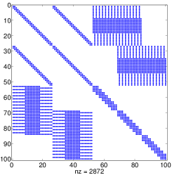
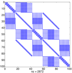
Figure 3: Sparsity patterns for the two-scale method with $N=27$. Left: ordered as in (3.9). Right: lexicographical ordering

To use the test harness, Test_FEM.m, to implement the two-scale method for our test problem, set the variable Method to two-scale on Line 18.

In 4(a) we present computed errors for various values of $N$, that are chosen, for simplicity, to be perfect cubes, which demonstrates that Theorem 3.4 holds in practice: the method is indeed first-order convergent in the energy norm. Moreover, the errors for the two-scale method are very similar to those of the classical method (the difference is to the order of 1%) even though far fewer degrees of freedom are used. For example, when $N=2^{12}$ the classical FEM has 16,769,025 degrees of freedom, compared with 122,625 for the two-scale method. However, comparing 1(b) and 4(b), we see that the nature of the point-wise errors are very different. We defer further comparisons between the methods to Section 5, where efficiency of the various methods is discussed in detail.

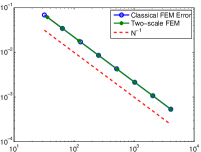
(a) Rate of convergence

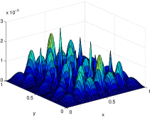
(b) $u-\widehat{u}_{64,64}$

Figure 4: Left: convergence of the classical and two-scale methods. Right: error in the two-scale solution with $N=64$ (right)

4 A multiscale sparse grid finite element method

We have seen that the two-scale method can match the accuracy of the classical FEM, even though only $\mathcal{O}(N^{4/3})$ degrees of freedom are used, rather than $\mathcal{O}(N^{2})$. We shall now see that it is possible to further reduce the required number of degrees of freedom to $\mathcal{O}(N\log N)$, again without sacrificing the accuracy of the method very much. The approach we present is equivalent, up to the choice of basis, to the hierarchical sparse grid method described by, for example, Bungartz and Griebel BuGr04 . But, because we present it as a generalisation of the two-scale method, we like to refer to it as the “multiscale” method.

Informally, the idea can be summarised in the following way. Suppose that $N=2^{k}$ for some $k$. For the two-scale method, we solved the problem (in a sense) on two overlapping grids: one with $N\times N^{1/3}$ intervals, and one with $N^{1/3}\times N$. Instead, we could apply the same algorithm, but on grids with $N\times(N/2)$ and $(N/2)\times N$ intervals respectively. Next we apply this same two-scale approach to each of these two grids, giving three overlapping grids with $N\times(N/4)$, $(N/2)\times(N/2)$, and $(N/4)\times N$ intervals. The process is repeated recursively, until the coarsest grids have $2$ intervals in one coordinate direction — the smallest feasible number.

More rigorously, we begin in Section 4.1 by constructing a multiscale interpolant, using an approach the authors presented in (RuMa14, , §3.1). This is then analysed in Section 4.2. As with the two-scale method, this leads to a FEM, described in 4.3. In Section 4.4 we show how this can be programmed, and present numerical results for our test problem.

Throughout the analysis, we use the following identities, which are easily established using, for example, inductive arguments.

Lemma 3

For any $k\geq 1$ we have the following identities

$$\begin{split}\displaystyle\sum\limits_{i=0}^{k-1}2^{i}=2^{k}-1,\qquad\text{ and }\qquad\displaystyle\sum\limits_{i=0}^{k-1}2^{-i}=2-2^{1-k}.\end{split}$$

4.1 The multiscale interpolant

Let $I_{N,N}$ denote the piecewise bilinear interpolation operator on $V_{N,N}$. Consider the following two-scale interpolation technique (3.3):

$$I^{(1)}_{N,N}=I_{N,\sigma(N)}+I_{\sigma(N),N}-I_{\sigma(N),\sigma(N)},$$ (4.1)

where $\sigma(N)$ is an integer that divides $N$. In particular, in Corollary 1, $\sigma(N)=CN^{1/3}$ is presented as a suitable choice. However, the same approach can be applied to, say, the terms $I_{N,\sigma(N)}$ and $I_{\sigma(N),N}$, and again recursively to the terms that emerge from that. Following the approach that is standard for multiscale sparse grid methods, we let $\sigma(N)=N/2$.

Let $I_{N_{x},N_{y}}$ denote the piecewise bilinear interpolation operator on $V_{N_{x},N_{y}}$. The corresponding Level 1 operator is

$$I^{(1)}_{N_{x},N_{y}}:=I_{N_{x},\frac{N_{y}}{2}}+I_{\frac{N_{x}}{2},N_{y}}-I_{\frac{N_{x}}{2},\frac{N_{y}}{2}}.$$ (4.2a)

The positively signed terms of (4.2a) are associated with spaces of dimension $$\mathcal{O}(N^{2}/2) \mathcal{O}(N^{2}/4)$$ while the negatively signed term is associated with a space of dimension . The Level 2 operator is obtained by applying the Level 1 operator to the positive terms in (4.2a), giving

$$I^{(2)}_{N,N}=I^{(1)}_{N,\frac{N}{2}}+I^{(1)}_{\frac{N}{2},N}-I_{\frac{N}{2},\frac{N}{2}}=I_{N,\frac{N}{4}}+I_{\frac{N}{2},\frac{N}{2}}+I_{\frac{N}{4},N}-I_{\frac{N}{2},\frac{N}{4}}-I_{\frac{N}{4},\frac{N}{2}}.$$ (4.2b)

Note that the right-hand side of this expression features three (positively signed) operators that map to subspaces of dimension $\mathcal{O}(N^{2}/4)$, and two (negatively signed) operators that map to subspaces of dimension $\mathcal{O}(N^{2}/8)$. To obtain the Level 3 operator, we again apply the Level 1 operator to the positive terms in (4.2b), because they are the ones associated with the larger spaces. In general, the Level $k$ operator is obtained by applying the Level 1 operator of (4.2a) to the positive terms in $I^{(k-1)}_{N,N}$. This leads to the following definition.

Definition 1 (Multiscale Interpolation Operator)

Let $I^{(0)}_{N,N}=I_{N,N}$ and, from (4.2a), let $I^{(1)}_{N,N}=I_{N,\frac{N}{2}}+I_{\frac{N}{2},N}-I_{\frac{N}{2},\frac{N}{2}}$. For $k=2,3,\dots$, let $I^{(k)}_{N,N}$ be obtained by applying the Level 1 operator in (4.2a) to the positively signed terms in $I^{(k-1)}_{N,N}$.

We now provide an explicit formula for $I^{(k)}_{N,N}$. This recovers a standard expression used, for example, in the combination technique outlined in PfZh99 .

Lemma 4

Let $I^{(k)}_{N,N}$ be the multiscale interpolation operator constructed in Definition 1 above. Then

$$I^{(k)}_{N,N}=\displaystyle\sum\limits_{i=0}^{k}I_{\frac{N}{2^{i}},\frac{N}{2^{k-i}}}-\displaystyle\sum\limits_{i=1}^{k}I_{\frac{N}{2^{i}},\frac{N}{2^{k+1-i}}},\qquad\text{ for }k=0,1,2,\dots.$$ (4.3)

Proof

It is easy to check that the formula (4.3) is consistent with the construction given in Definition 1 for $k=0$ and $k=1$.

Next, assume that (4.3) holds for an arbitrary $k=n$; that is,

$$I^{(n)}_{N,N}=\displaystyle\sum\limits_{i=0}^{n}I_{\frac{N}{2^{i}},\frac{N}{2^{n-i}}}-\displaystyle\sum\limits_{i=1}^{n}I_{\frac{N}{2^{i}},\frac{N}{2^{n+1-i}}}.$$ (4.4)

Following Definition 1, apply the Level 1 operator (4.2a) to each term in the first sum of the right-hand side of (4.4). This gives

$$I_{N,N}^{(n+1)}=\displaystyle\sum\limits_{i=0}^{n}\left[I_{\frac{N}{2^{i}},\frac{N}{2^{n+1-i}}}+I_{\frac{N}{2^{i+1}},\frac{N}{2^{n-i}}}-I_{\frac{N}{2^{i+1}},\frac{N}{2^{n+1-i}}}\right]-\displaystyle\sum\limits_{i=1}^{n}I_{\frac{N}{2^{i}},\frac{N}{2^{n+1-i}}}\\ =I_{\frac{N}{2^{n+1}},N}+\displaystyle\sum\limits_{i=0}^{n}\left[I_{\frac{N}{2^{i}},\frac{N}{2^{n+1-i}}}-I_{\frac{N}{2^{i+1}},\frac{N}{2^{n+1-i}}}\right]\\ =\displaystyle\sum\limits_{i=0}^{n+1}I_{\frac{N}{2^{i}},\frac{N}{2^{n+1-i}}}-\displaystyle\sum\limits_{i=1}^{n+1}I_{\frac{N}{2^{i}},\frac{N}{2^{n+2-i}}}.$$

That is, (4.3) holds for $k=n+1$, as required.

Although (4.3) is a succinct representation of the multiscale interpolation operator, for the purposes of analysis we are actually interested in the difference between operators at successive levels. First consider the difference between the interpolation operators at Levels 0 and 1:

$$I^{(0)}_{N,N}-I^{(1)}_{N,N}=I_{N,N}-I_{N,\frac{N}{2}}-I_{\frac{N}{2},N}+I_{\frac{N}{2},\frac{N}{2}}.$$

Recalling (3.2a) and (3.4), this expression can be written as

$$I^{(0)}_{N,N}-I^{(1)}_{N,N}=(I_{N,0}\circ I_{0,N})-(I_{N,0}\circ I_{0,\frac{N}{2}})-(I_{\frac{N}{2},0}\circ I_{0,N})+(I_{\frac{N}{2},0}\circ I_{0,\frac{N}{2}})\\ =\left(I_{N,0}-I_{\frac{N}{2},0}\right)\left(I_{0,N}-I_{0,\frac{N}{2}}\right),$$ (4.5)

an identity used repeatedly in LMSZ09 . One can derive a similar expression $I^{(1)}_{N,N}-I^{(2)}_{N,N}$:

$$I^{(1)}_{N,N}-I^{(2)}_{N,N}=I_{N,\frac{N}{2}}+I_{\frac{N}{2},N}-I_{\frac{N}{2},\frac{N}{2}}-I_{N,\frac{N}{4}}-I_{\frac{N}{2},\frac{N}{2}}-I_{\frac{N}{4},N}+I_{\frac{N}{2},\frac{N}{4}}+I_{\frac{N}{4},\frac{N}{2}}.$$

Invoking (3.2a) and simplifying we get

$$I^{(1)}_{N,N}-I^{(2)}_{N,N}= (I_{N,0}\circ I_{0,\frac{N}{2}})+(I_{\frac{N}{2},0}\circ I_{0,N})-(I_{\frac{N}{2},0}\circ I_{0,\frac{N}{2}})-(I_{N,0}\circ I_{0,\frac{N}{4}})$$

$$-(I_{\frac{N}{2},0}\circ I_{0,\frac{N}{2}})-(I_{\frac{N}{4},0}\circ I_{0,N})+(I_{\frac{N}{2},0}\circ I_{0,\frac{N}{4}})+(I_{\frac{N}{4},0}\circ I_{0,\frac{N}{2}}),$$

$$=\left(I_{N,0}-I_{\frac{N}{2},0}\right)\left(I_{0,\frac{N}{2}}-I_{0,\frac{N}{4}}\right)+\left(I_{\frac{N}{2},0}-I_{\frac{N}{4},0}\right)\left(I_{0,N}-I_{0,\frac{N}{2}}\right).$$

We now give the general form for the representation of the difference between operators at successive levels in terms of one-dimensional operators. The resulting identity is an important tool in our analysis of the bound on the error for the multiscale interpolation operator.

Lemma 5

Let $I^{(k)}_{N,N}$ be the multiscale interpolation operator defined in (4.3). Then, for $k=0,1,2,\dots$,

$$I^{(k-1)}_{N,N}-I^{(k)}_{N,N}=\displaystyle\sum\limits_{i=0}^{k-1}\left(I_{\frac{N}{2^{i}},0}-I_{\frac{N}{2^{i+1}},0}\right)\left(I_{0,\frac{N}{2^{k-1-i}}}-I_{0,\frac{N}{2^{k-i}}}\right).$$ (4.6)

Proof

From the expression for the multiscale operator in (4.3) we can write

$$I^{(k-1)}_{N,N}-I^{(k)}_{N,N}=\displaystyle\sum\limits_{i=0}^{k-1}I_{\frac{N}{2^{i}},\frac{N}{2^{k-1-i}}}-\displaystyle\sum\limits_{i=1}^{k-1}I_{\frac{N}{2^{i}},\frac{N}{2^{k-1}}}-\displaystyle\sum\limits_{i=0}^{k}I_{\frac{N}{2^{i}},\frac{N}{2^{k-i}}}+\displaystyle\sum\limits_{i=1}^{k}I_{\frac{N}{2^{i}},\frac{N}{2^{k+1-i}}}\\ =\displaystyle\sum\limits_{i=0}^{k-1}I_{\frac{N}{2^{i}},\frac{N}{2^{k-1-i}}}-\left(\displaystyle\sum\limits_{i=0}^{k-1}I_{\frac{N}{2^{i}},\frac{N}{2^{k-i}}}-I_{N,\frac{N}{2^{k}}}\right)-\left(\displaystyle\sum\limits_{i=0}^{k-1}I_{\frac{N}{2^{i}},\frac{N}{2^{k-i}}}+I_{\frac{N}{2^{k}},N}\right)+\displaystyle\sum\limits_{i=0}^{k-1}I_{\frac{N}{2^{i+1}},\frac{N}{2^{k-i}}}\\ =\displaystyle\sum\limits_{i=0}^{k-1}\left(I_{\frac{N}{2^{i}},\frac{N}{2^{k-1-i}}}-I_{\frac{N}{2^{i}},\frac{N}{2^{k-i}}}+I_{\frac{N}{2^{i+1}},\frac{N}{2^{k-i}}}\right)-\displaystyle\sum\limits_{i=0}^{k-1}I_{\frac{N}{2^{i}},\frac{N}{2^{k-i}}}+I_{N,\frac{N}{2^{k}}}-I_{\frac{N}{2^{k}},N}\\ =\displaystyle\sum\limits_{i=0}^{k-1}\left(I_{\frac{N}{2^{i}},\frac{N}{2^{k-1-i}}}-I_{\frac{N}{2^{i}},\frac{N}{2^{k-i}}}+I_{\frac{N}{2^{i+1}},\frac{N}{2^{k-i}}}\right)-\displaystyle\sum\limits_{i=0}^{k-1}I_{\frac{N}{2^{i+1}},\frac{N}{2^{k-1-i}}}\\ =\displaystyle\sum\limits_{i=0}^{k-1}\left(I_{\frac{N}{2^{i}},\frac{N}{2^{k-1-i}}}-I_{\frac{N}{2^{i}},\frac{N}{2^{k-i}}}+I_{\frac{N}{2^{i+1}},\frac{N}{2^{k-i}}}-I_{\frac{N}{2^{i+1}},\frac{N}{2^{k-1-i}}}\right),$$

which, recalling (4.5), gives the desired expression.

4.2 Analysis of the multiscale interpolation operator

In this section we provide an analysis for the error incurred by the multiscale interpolant. Standard finite element analysis techniques then provide a full analysis of the underlying method. We begin by establishing a bound, in the energy norm, for the difference between interpolants at successive levels.

Theorem 4.1

Suppose $\Omega=(0,1)^{2}$. Let $u\in H^{1}_{0}(\Omega)$ and $I^{(k)}_{N,N}$ be the multi-scale interpolation operator defined in (4.3). Then there exists a constant, $C$, independent of $N$ and $k$, such that

$$\|I^{(k)}_{N,N}u-I^{(k-1)}_{N,N}u\|_{B}\leq C(k4^{k+1}N^{-4}+4^{k+1}N^{-3}).$$

Proof

By stating $\|I_{N,N}^{(k)}u-I_{N,N}^{(k-1)}u\|_{0,\Omega}$ in the form of Lemma 5 and applying the triangle inequality, along with the first inequality in (3.1) and Lemma 3 we see

$$\|I_{N,N}^{(k)}u-I_{N,N}^{(k-1)}u\|_{0,\Omega}=\left\|\displaystyle\sum\limits_{i=0}^{k-1}(I_{\frac{N}{2^{i}},0}-I_{\frac{N}{2^{i+1}},0})(I_{0,\frac{N}{2^{k-1-i}}}-I_{0,\frac{N}{2^{k-i}}})u\right\|_{0,\Omega}\\ \leq C\displaystyle\sum\limits_{i=0}^{k-1}\left(\frac{N}{2^{i+1}}\right)^{-2}\left\|\left(I_{0,\frac{N}{2^{k-1-i}}}-I_{0,\frac{N}{2^{k-i}}}\right)\frac{\partial^{2}u}{\partial x^{2}}\right\|_{0,\Omega}\\ \leq C\displaystyle\sum\limits_{i=0}^{k-1}\left(\frac{N}{2^{i+1}}\right)^{-2}\left(\frac{N}{2^{k-i}}\right)^{-2}\left\|\frac{\partial^{4}u}{\partial x^{2}\partial y^{2}}\right\|_{0,\Omega}\\ \leq C\displaystyle\sum\limits_{i=0}^{k-1}(2^{2i+2})(2^{2k-2i})N^{-4}=Ck4^{k+1}N^{-4}.$$ (4.7)

Using a similar argument, but with the second inequality in (3.1), we have

$$\left\|\frac{\partial}{\partial x}\left(\displaystyle\sum\limits_{i=0}^{k-1}(I_{\frac{N}{2^{i}},0}-I_{\frac{N}{2^{i+1}},0})(I_{0,\frac{N}{2^{k-1-i}}}-I_{0,\frac{N}{2^{k-i}}})u\right)\right\|_{0,\Omega}\\ \leq C_{0}\displaystyle\sum\limits_{i=0}^{k-1}\left(\frac{N}{2^{i+1}}\right)^{-1}\left\|(I_{0,\frac{N}{2^{k-1-i}}}-I_{0,\frac{N}{2^{k-i}}})\frac{\partial^{2}u}{\partial x^{2}}\right\|_{0,\Omega}\leq C4^{k+1}N^{-3}.$$ (4.8)

The corresponding bound on the $y$-derivatives is obtained in a similar manner. Combining these results gives

$$\|\nabla(I^{(k)}_{N,N}u-I^{(k-1)}_{N,N}u)\|_{0,\Omega}\leq C4^{k+1}N^{-3}.$$

Now following from the definition of the energy norm and results (4.7) and (4.8) one has

$$\|I^{(k)}_{N,N}u-I^{(k-1)}_{N,N}u\|_{B}\leq\|\nabla(I^{(k)}_{N,N}u-I^{(k-1)}_{N,N}u)\|_{0,\Omega}+\|I^{(k)}_{N,N}u-I^{(k-1)}_{N,N}u\|_{0,\Omega}\\ \leq C4^{k+1}N^{-3}+Ck4^{k+1}N^{-4}.$$

We now want to show that $\|I^{(k)}_{N,N}u-I^{(k-1)}_{N,N}u\|_{B}$ is an upper bound for $\|I^{(k-1)}_{N,N}u-I_{N,N}u\|_{B}$, thus showing that in, order to estimate $\|I_{N,N}u-I^{(k)}_{N,N}u\|_{B}$, it is enough to look at $\|I^{(k)}_{N,N}u-I^{(k-1)}_{N,N}u\|_{B}$.

Lemma 6

Let $u$ and $I^{(k)}_{N,N}$ be defined as in Theorem 4.1. Then there exists a constant, $C$, independent of $N$ and $k$, such that

$$\|I^{(k-1)}_{N,N}u-I_{N,N}u\|_{B}\leq\|I^{(k)}_{N,N}u-I^{(k-1)}_{N,N}u\|_{B}.$$

Proof

Taking the result of Theorem 4.1 and by applying an inductive argument one can easily deduce that

$$\sum\limits_{i=1}^{k-1}i4^{i+1}\leq k4^{k+1}\quad\text{ and }\quad\displaystyle\sum\limits_{i=1}^{k-1}4^{i+1}\leq 4^{k+1}.$$

The result then follows by applying the triangle inequality and observing that

$$\sum\limits_{i=1}^{k-1}\|I^{(i)}_{N,N}u-I^{(i-1)}_{N,N}u\|_{B}\leq\displaystyle\sum\limits_{i=1}^{k-1}(i4^{i+1}N^{-4}+4^{i+1}N^{-3}).$$

Lemma 7

Let $u$ and $I^{(k)}_{N,N}$ be defined as in Theorem 4.1. Then there exists a constant, $C$, independent of $N$ and $k$, such that

$$\|I^{(k)}_{N,N}u-I_{N,N}u\|_{B}\leq C4^{k+1}N^{-3}.$$

Proof

By the triangle inequality and the results of Theorem 4.1 and Lemma 6 one has

$$\|I^{(k)}_{N,N}u-I_{N,N}u\|_{B}\leq\|I^{(k)}_{N,N}u-I^{(k-1)}_{N,N}u\|_{B}+\|I^{(k-1)}_{N,N}u-I_{N,N}u\|_{B}\\ \leq C(k4^{k+1}N^{-4}+4^{k+1}N^{-3}).$$

The result now follows by noting that, for $k\leq N$ (which will always be the case),

$$4^{k+1}N^{-3}\geq k4^{k+1}N^{-4}.$$

Using the triangle inequality, we combined this result with 2 and 7 to establish the following error estimate.

Theorem 4.2

Let $u$ and $I^{(k)}_{N,N}$ be defined as in Theorem 4.1. Then there exists a constant, $C$, independent of $N$ and $k$, such that

$$\|u-I^{(k)}_{N,N}u\|_{B}\leq C(N^{-1}+4^{k+1}N^{-3}).$$

Remark 2

Our primary goal is to construct an efficient finite element method, by taking the smallest possible space on which $I^{(k)}_{N,N}u$ can be defined. Thus we want to take $k$ as large as is possible while retaining the accuracy of the underlying method. On a uniform mesh the coarsest grid must have at least two intervals in each coordinate direction. From (4.3) it is clear that the coarsest grid we interpolate over has $N/2^{k}$ intervals. Thus the largest and most useful value of $k$ we can choose is $\widetilde{k}=\log_{2}N-1$. In light of this, we have the following result.

Corollary 2

Let $u$ and $I^{(\widetilde{k})}_{N,N}$ be defined as in Theorem 4.1. Taking $k:=\widetilde{k}=\log_{2}(N)-1$ in Theorem 4.2, there exists a constant, $C$, independent of $N$, such that

$$\|u-I^{(\widetilde{k})}_{N,N}u\|_{B}\leq CN^{-1}.$$

4.3 Multiscale sparse grid finite element method

Let $\psi_{i}^{N}$ and $\psi_{j}^{N}$ be as defined in (2.2) We now define the finite dimensional space $V^{(k)}_{N,N}\subset H^{1}_{0}(\Omega)$ as

$$V^{(k)}_{N,N}=\mathrm{span}\left\{\psi^{N}_{i}(x)\psi^{N/2^{k}}_{j}(y)\right\}^{i=1:N-1}_{j=1:N/2^{k}-1}\\ +\mathrm{span}\left\{\psi^{N/2}_{i}(x)\psi^{N/2^{k-1}}_{j}(y)\right\}^{i=1:N/2-1}_{j=1:N/2^{k-1}-1}\\ +\cdots+\mathrm{span}\left\{\psi^{N/2^{k-1}}_{i}(x)\psi^{N/2}_{j}(y)\right\}^{i=1:N/2^{k-1}-1}_{j=1:N/2-1}+\mathrm{span}\left\{\psi^{N/2^{k}}_{i}(x)\psi^{N}_{j}(y)\right\}^{i=1:N/2^{k}-1}_{j=1:N-1}.$$

Note that each two dimensional basis function is the product of two one-dimensional functions that are of different scales. This description involves $(k+1)2^{-k}N^{2}+(2^{-k+1}-4)N+k+1$ functions in the spanning set, which are illustrated in the diagrams in Figure 5. The left most diagram shows a uniform mesh with $N=16$ intervals in each coordinate direction. Each node represents a basis function for the space $V^{(0)}_{N,N}=V_{N,N}$.

Figure 5: Meshes for the multiscale method for $N=16$, based on the spaces (left to right) $V^{(0)}_{N,N}$, $V^{(1)}_{N,N}$ and $V^{(2)}_{N,N}$

In the centre column of Figure 5 we show the grids associated with $V^{(1)}_{N,N}$. Notice that the spaces associated with these two grids are not linearly independent. To form an invertible system matrix, in Figure 5 we highlight a particular choice of non-redundant basis functions by solid circles:

$$\left\{\psi^{N}_{i}(x)\psi^{N/2}_{j}(y)\right\}^{i=1:2:N-1}_{j=1:N/2-1}\quad\text{ and }\quad\left\{\psi^{N/2}_{i}(x)\psi^{N}_{j}(y)\right\}^{i=1:N/2-1}_{j=1:N-1}.$$

The right-most column of Figure 5 show the grids associated with $V^{(2)}_{N,N}$. Again we use solid circles to represent our choice of basis:

$$\left\{\psi^{N}_{i}(x)\psi^{N/4}_{j}(y)\right\}^{i=1:2:N-1}_{j=1:N/4-1},\quad\left\{\psi^{N/2}_{i}(x)\psi^{N/2}_{j}(y)\right\}^{i=1:N/2-1}_{j=1:N/2-1},\\ \text{ and }\quad\left\{\psi^{N/4}_{i}(x)\psi^{N}_{j}(y)\right\}^{i=1:N/4-1}_{j=1:2:N-1}.$$

There are many ways in which one can choose which basis functions to include. The way we have chosen, excluding the boundary, is as follows:

• when $N_{x}>N_{y}$ include every second basis function in the $x$-direction;

• when $N_{x}=N_{y}$ or when $2N_{x}=N_{y}$ include all basis functions;

• from the remaining subspaces include every second basis function in the $y$-direction.

In general the choice of basis we make for the space $V^{(k)}_{N,N}$ is dependent on whether $k$ is odd or even. When $k$ is odd the basis we choose is:

$$\bigcup\limits_{l=0}^{(k-1)/2}\left\{\psi_{i}^{N/2^{l}}\psi_{j}^{N/2^{k-l}}\right\}^{i=1:2:N/2^{l}-1}_{j=1:N/2^{k-l}-1}\bigcup\left\{\psi_{i}^{N/2^{(k+1)/2}}\psi_{j}^{N/2^{(k-1)/2}}\right\}^{i=1:N/2^{(k+1)/2}-1}_{j=1:N/2^{(k-1)/2}-1}\\ \bigcup\limits_{l=(k+3)/2}^{k}\left\{\psi_{i}^{N/2^{l}}\psi_{j}^{N/2^{k-l}}\right\}^{i=1:N/2^{l}-1}_{j=1:2:N/2^{k-l}-1};$$ (4.9a)

And when $$k$$ is even the basis we choose is:

$$\bigcup\limits_{l=0}^{k/2-1}\left\{\psi_{i}^{N/2^{l}}\psi_{j}^{N/2^{k-l}}\right\}^{i=1:2:N/2^{l}-1}_{j=1:N/2^{k-l}-1}\bigcup\left\{\psi_{i}^{N/2^{k/2}}\psi_{j}^{N/2^{k/2}}\right\}^{i=1:N/2^{k/2}-1}_{j=1:N/2^{k/2}-1}\\ \bigcup\limits_{l=k/2+1}^{k}\left\{\psi_{i}^{N/2^{l}}\psi_{j}^{N/2^{k-l}}\right\}^{i=1:N/2^{l}-1}_{j=1:2:N/2^{k-l}-1}.$$ (4.9b)

This has dimension $2^{-k}(k/2+1)N^{2}-2N+1$. For a computer implementation one can, of course, choose alternative ways of expressing the basis. Although these are mathematically equivalent, they can lead to different linear systems. We can now formulate the multiscale sparse grid finite element method: find $u_{N,N}^{(k)}\in{V}_{N,N}^{(k)}$ such that

$$\mathcal{B}(u_{N,N}^{(k)},v_{N,N})=(f,v_{N,N})\quad\text{ for all }v_{N,N}\in{V}^{(k)}_{N,N}.$$ (4.10)

We will consider the analysis for the case $k:=\widetilde{k}=\log_{2}N-1$.

Theorem 4.3

Let $u$ be the solution to (1.1), and $u_{N,N}^{(\widetilde{k})}$ the solution to (4.10). Then there exists a constant $C$, independent of $N$ and $\varepsilon$, such that

$$\|u-u^{(\widetilde{k})}_{N,N}\|_{B}\leq CN^{-1}.$$

Proof

The bilinear form (4.10) is continuous and coercive, so it follows from classical finite element analysis that

$$\|u-u^{(\widetilde{k})}_{N,N}\|_{B}\leq C\displaystyle\inf_{\psi\in V^{(\widetilde{k})}_{N,N}(\Omega)}\|u-\psi\|_{B}.$$

Since $I^{(k)}_{N,N}u\in V^{(\widetilde{k})}_{N,N}(\Omega)$ the result is an immediate consequence of Corollary 2.

4.4 Implementation of the multiscale method

We now turn to the construction of the linear system for the method (4.10). As with the construction of the linear system for (3.8), we begin by building matrices that project from the one-dimensional subspaces of $V_{N}$ to the full one-dimensional space $V_{N}$. In MATLAB this is done with the following line of code

⬇

px = sparse(interp1(Sx, eye(length(Sx)), x));

where $x$ is a uniform mesh on $[0,1]$ with $N$ intervals, and $S_{x}$ is a submesh of $x$ with $N/M$ intervals and $M$ is a proper divisor of $N$.

Next we build a collection of two-dimensional projection matrices, $P$. Each of these projects a bilinear function expressed in terms of each of the basis functions in (4.9), to one in $V_{N,N}$. This is done using MultiScale_Projector.m, a function written in MATLAB, and the following piece of code:

⬇

P = kron(py(2:N,2:skip_y:My), px(2:N,2:skip_x:Mx));

Here $M_{x}$ and $M_{y}$ are the number of intervals in the coarse $x$- and $y$-directions respectively. The values $skip_{x}$ and $skip_{y}$ are set to either $1$ or $2$ depending on whether we include all basis functions, or every other basis function, in (4.9). The projectors in the collection are concatenated to give the projector from $V^{(k)}_{N,N}$ to $U_{N,N}$ That is $P=(P_{1}|P_{2}|\dots|P_{k}|P_{k+1})$.

As is the case with the two-scale method, having constructed $P$ and given the linear system for the classical Galerkin method, $Au_{N,N}=b$, the linear system for the multiscale method is $(P^{T}AP)u^{(k)}_{N,N}=P^{T}b$. Evaluating $Pu^{(k)}_{N,N}$ then projects the solution back to the original space $V_{N,N}$.

To use the test harness, Test_FEM.m, to implement the multiscale method for our test problem, set the variable Method to multiscale on Line 18.

In 6(a) we present numerical results for the multiscale method which demonstrate that, in practice, the $CN^{-1}$ term from the theoretical results of Theorem 4.3 is observed numerically. The errors for the multiscale method are very similar to those of the classical Galerkin method and the two-scale method, however the degrees of freedom are greatly reduced. We saw in Section 3.3, that for $N=2^{12}$ the classical Galerkin FEM involves $16,769,025$ degrees of freedom, compared to $122,625$ for the two-scale method. This is further reduced to $45,057$ degrees of freedom for the multiscale method (taking $k=\log_{2}N-1$). Again comparing 1(b), 4(b) and 6(b) we see that although the nature of the point-wise errors are quite different, they are all similar in magnitude.

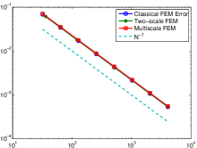
(a) Rate of convergence

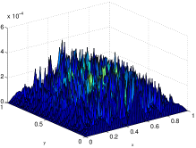
(b) $u-u_{64,64}^{(5)}$

Figure 6: Left: the convergence of the classical, two-scale and multiscale methods. Right: error in the multiscale solution with $N=64$ and $k=5$

4.5 Hierarchical basis

The standard choice of basis used in the implementation of a sparse grid method is generally the hierarchical basis (Yser86 ), which is quite different from that given in (4.9). The most standard reference for sparse grids is the work of Bungartz and Griebel BuGr04 , so we adopt their notation.

The hierarchical basis for the (full) space $V_{N,N}(\Omega)$, is

$$\bigoplus_{m,n=1,\dots,\log_{2}N}W_{m,n},\quad\text{ where }\quad W_{m,n}=\left\{\psi^{2^{m}}_{i}\psi^{2^{n}}_{j}\right\}^{i=1:2:2^{m}-1}_{j=1:2:2^{n}-1}.$$ (4.11)

This is shown in Figure 7 for the case $N=8$. The hierarchical basis is constructed from $9$ subspaces. Recall that each dot on these grids represents a basis function with support on the adjacent four rectangles. For example, $W_{11}$ is shown in the top left, and represents a simple basis function with support on the whole domain. In the subspace $W_{33}$ in the bottom right of Figure 7 each basis function has support within the rectangle on which it is centred. No two basis functions in a given subspace share support within that subspace.

\begin{picture}(4866.0,5670.0)(43.0,-2473.0)\end{picture}

Figure 7: Left: All subspaces required to build a hierarchical basis for a full grid where $N=8$. Right: Full grid with basis functions for $N=8$.

A sparse grid method is constructed by omitting a certain number of the subspaces $W_{m,n}$ in (4.11). For a typical problem, one uses only those subspaces $W_{m,n}$ for which $m+n\leq\log_{2}N+1$: compare Figures 3.3 and 3.5 of BuGr04 . This gives the same spaces as defined by (4.9), taking $k=\log_{2}N-1$. Expressed in terms of a hierarchical basis, the basis for $V^{(k)}_{N,N}$ is written as

$$\bigoplus_{\begin{subarray}{c}m,n=1,\dots,\log_{2}N\\ m+n\leq\log_{2}N+1\end{subarray}}W_{m,n}.$$ (4.12)

Both choices give rise to basis functions centred at the same grid points (but with different support) and have linear systems of the same size, but different structure: see Figure 9 and Figure 10.

\begin{picture}(4920.0,6045.0)(43.0,-2848.0)\end{picture}

Figure 8: Left: All subspaces required to build a hierarchical basis for a sparse grid where $N=8$. Right: Sparse grid with basis functions for $N=8$.

It is known that this basis leads to reduced sparsity of the linear system (see, e.g., (HGCh07, , p. 250)). Numerical experiments have shown that the basis given in (4.9) leads to fewer non-zeros entries in the system matrix, and so is our preferred basis. In Figure 9 we compare the sparsity pattern of the system matrices for the basis described in (4.9) for the case $N=32$ using a natural ordering (left) and lexicographical ordering (right). For the same value of $N$, Figure 10 shows the sparsity patterns for the system matrices constructed using the hierarchical basis (4.12), again using natural and lexicographical ordering. The matrices in Figure 10 contain more nonzero entries and are much denser than those in Figure 9.

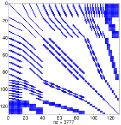
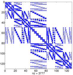
Figure 9: Sparsity patterns for the multiscale method using the basis in (4.9) with $N=32$. Left: unknowns ordered as (4.9). Right: lexicographical ordering.

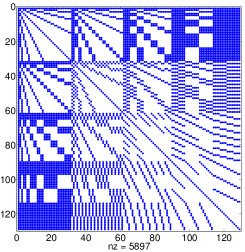
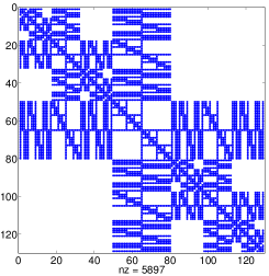
Figure 10: Sparsity patterns using a hierarchical basis (4.12) with $N=32$. Left: unknowns ordered as in (4.12). Right: lexicographical ordering.

5 Comparison of three FEMs

In 6(a) we presented results that demonstrated that the three methods achieve similar levels of accuracy. We now wish to quantify if, indeed, the sparse grid methods are more efficient than the classical method. To do this in a thorough fashion would require a great deal of effort to

• investigate efficient storage of matrices arising from these specialised grids;

• investigate the design of suitable preconditioners for iterative techniques, or Multigrid methods.

These topics are beyond the scope of this article. Instead, we apply a direct solver, since it is the simplest possible “black-box” solver and avoids concerns involving preconditioners and stopping criteria. Therefore we compare the methods with respect to the wall-clock time taken by MATLAB’s “backslash” solver. Observing the diagnostic information provided (spparms(’spumoni’,1)), we have verified that this defaults to the CHOLMOD solver for symmetric positive definite matrices Davi08 .

The results we present were generated on a single node of a Beowulf cluster, equipped with 32 Mb RAM and two AMD Opteron 2427, 2200 MHz processors, each with 6 cores. The efficiency of parallelised linear algebra routines can be highly dependent on the matrix structure. Therefore we present results obtained both using all 12 cores, and using a single core (enforced by launching MATLAB with the -singleCompThread option). All times reported are in seconds, and have been averaged over three runs.

In Table 1 we can see that, for $N=2^{12}$, over a thousand seconds are required to solve the system for the classical method on a single core, and 560 seconds with all 12 cores enabled. (It is notable, that, for smaller problems, the solver was more efficient when using just 1 core).

When the two-scale method is used, Table 1 shows that there is no great loss of accuracy, but solve times are reduced by a factor of 3 on 1 core and (roughly) a factor of 5 on 12 cores. Employing the multiscale method, we see a speed-up of (roughly) 7 on one core, and 15 on 12 cores.

Table 1: Comparing efficiency of the classical, two-scale, and multiscale FEMs

	Classical Galerkin
$N$	512	1024	2048	4096
Error	4.293e-03	2.147e-03	1.073e-03	5.346e-04
Solver Time (1 core)	3.019	18.309	134.175	1161.049
Solver Time (12 cores)	6.077	26.273	119.168	562.664
Degrees of Freedom	261,121	1,046,529	4,190,209	16,769,025
Number of Non-zeros	2,343,961	9,406,489	37,687,321	150,872,089
	Two-scale method
$N$	512	1000	2197	4096
Error	4.668e-03	2.383e-03	1.082e-03	5.796e-04
Solver Time (1 core)	0.806	4.852	43.702	281.838
Solver Time (12 cores)	0.810	3.274	21.448	105.727
Degrees of Freedom	7,105	17,901	52,560	122,625
Number of Non-zeros	1,646,877	6,588,773	33,234,032	118,756,013
	Multiscale method
$N$	512	1024	2048	4096
Error	4.437e-03	2.219e-03	1.109e-03	5.529e-04
Solver Time (1 core)	0.370	2.280	20.692	150.955
Solver Time (12 cores)	0.384	1.665	7.464	36.469
Degrees of Freedom	4,097	9,217	20,481	45,057
Number of Non-zeros	996,545	3,944,897	15,525,569	61,585,473

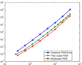
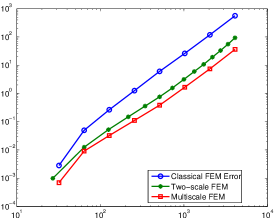
Figure 11: Solve time, in seconds, for linear systems using a direct solver on 1 core (left) and 12 cores (right)

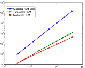
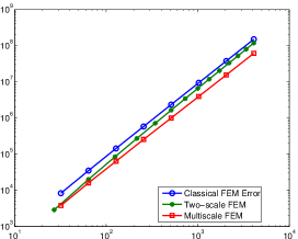
Figure 12: The number of degrees of freedom (left) and non-zero entries in the system matrices (right)

6 Conclusions

There are many published papers on the topic of sparse grid methods, particularly over the last two decades. Often though, they deal with highly specialized problems, and the analysis tends to be directed at readers that are highly knowledgeable in the fields of PDEs, FEMs, and functional analysis. Here we have presented a style of analysing sparse grid methods in a way that is accessible to a more general audience. We have also provided snippets of code and details on how to implement these methods in MATLAB.

The methods presented are not new. However, by treating the usual multiscale sparse grid method as a generalization of the two-scale method, we have presented a conceptually simple, yet rigorous, way of understanding and analysing it.

Here we have treated just a a simple two-dimensional problem on a uniform mesh. However, this approach has been employed to analyse sparse grid methods for specialised problems whose solutions feature boundary layers, and that are solved on layer-adapted meshes, see RuMa14 ; RuMa15 .

More interesting generalisations are possible, but the most important of these is to higher dimensional problems. An exposition of the issues involved is planned.

Acknowledgements

The work of Stephen Russell is supported by a fellowship from the College of Science at the National University of Ireland, Galway. The simple approach in (2.10) in determining the error was shown to us by Christos Xenophontos.

References

- [1] Susanne C. Brenner and Ridgway L. Scott. The mathematical theory of finite element methods. 3rd ed. Texts in Applied Mathematics 15. New York, NY: Springer. xvii, 397 p., 2008.
- [2] William L. Briggs, Van Emden Henson, and Steve F. McCormick. A multigrid tutorial. Society for Industrial and Applied Mathematics (SIAM), Philadelphia, PA, second edition, 2000.
- [3] Hans-Joachim Bungartz and Michael Griebel. Sparse grids. Acta Numer., 13:147–269, 2004.
- [4] Yanqing Chen, Timothy A. Davis, William W. Hager, and Sivasankaran Rajamanickam. Algorithm 887: CHOLMOD, supernodal sparse Cholesky factorization and update/downdate. ACM Trans. Math. Software, 35(3):Art. 22, 14, 2008.
- [5] T. A. Driscoll, N. Hale, and L. N. Trefethen (eds). Chebfun Guide. Pafnuty Publications, Oxford, 2014.
- [6] Tobin A. Driscoll. Learning MATLAB. Society for Industrial and Applied Mathematics (SIAM), Philadelphia, PA, 2009.
- [7] Mark S. Gockenbach. Understanding and implementing the finite element method. Society for Industrial and Applied Mathematics (SIAM), Philadelphia, PA, 2006.
- [8] Christian Grossmann and Hans-Görg Roos. Numerical treatment of partial differential equations. Universitext. Springer, Berlin, 2007. Translated and revised from the 3rd (2005) German edition by Martin Stynes.
- [9] Markus Hegland, Jochen Garcke, and Vivien Challis. The combination technique and some generalisations. Linear Algebra Appl., 420(2-3):249–275, 2007.
- [10] Desmond J. Higham and Nicholas J. Higham. MATLAB guide. Society for Industrial and Applied Mathematics (SIAM), Philadelphia, PA, second edition, 2005.
- [11] Alan J. Laub. Matrix analysis for scientists & engineers. Society for Industrial and Applied Mathematics (SIAM), Philadelphia, PA, 2005.
- [12] Qun Lin, Ningning Yan, and Aihui Zhou. A sparse finite element method with high accuracy. I. Numer. Math., 88(4):731–742, 2001.
- [13] Fang Liu, Niall Madden, Martin Stynes, and Aihui Zhou. A two-scale sparse grid method for a singularly perturbed reaction-diffusion problem in two dimensions. IMA J. Numer. Anal., 29(4):986–1007, 2009.
- [14] N. Madden and S. Russell. A multiscale sparse grid finite element method for a two-dimensional singularly perturbed reaction-diffusion problem. Adv. Comput. Math., (to appear).
- [15] Cleve B. Moler. Numerical computing with MATLAB. Society for Industrial and Applied Mathematics, Philadelphia, PA, 2004.
- [16] Octave community. GNU Octave 3.8.1, 2014.
- [17] C. Pflaum and A. Zhou. Error analysis of the combination technique. Numer. Math., 84(2):327–350, 1999.
- [18] Stephen Russell and Niall Madden. A multiscale sparse grid technique for a two-dimensional convection-diffusion problem with exponential layers. Lect. Notes Comput. Sci. Eng. Springer, Berlin, 2015, to appear.
- [19] Endre Süli and David F. Mayers. An introduction to numerical analysis. Cambridge University Press, Cambridge, 2003.
- [20] Harry Yserentant. On the multilevel splitting of finite element spaces. Numer. Math., 49(4):379–412, 1986.