Modelling aperiodic X-ray variability in black hole binaries as propagating mass accretion rate fluctuations: a short review

Abstract

Black hole binary systems can emit very bright and rapidly varying X-ray signals when material from the companion accretes onto the black hole, liberating huge amounts of gravitational potential energy. Central to this process of accretion is turbulence. In the propagating mass accretion rate fluctuations model, turbulence is generated throughout the inner accretion flow, causing fluctuations in the accretion rate. Fluctuations from the outer regions propagate towards the black hole, modulating the fluctuations generated in the inner regions. Here, I present the theoretical motivation behind this picture before reviewing the array of statistical variability properties observed in the light curves of black hole binaries that are naturally explained by the model. I also discuss the remaining challenges for the model, both in terms of comparison to data and in terms of including more sophisticated theoretical considerations.

1 Introduction

Black hole binaries display variability in their X-ray light curves on a wide range of timescales. On the longest timescales ($\sim$weeks to months), their spectrum evolves dramatically from being dominated by a hard power law in the hard state, to being dominated by a quasi-thermal accretion disk in the soft state (Tananbaum et al 1972; Done, Gierlinski & Kubota 2007). These spectral changes can be illustrated using a hardness intensity diagram (HID: Homan et al 2001; Belloni et al 2005). The x-axis is hardness, typically defined as the ratio of photon counts in the $16-20$ keV and $2-6$ keV bands of the Rossi X-ray Timing Explorer (RXTE), and the y-axis is intensity, typically defined as counts in the full RXTE band. This has the advantage of being completely model independent and it also allows a large amount of information to be condensed into a single plot. That the definitions are rather married to RXTE is a symptom of just how large a fraction of the available data is from that particular mission. Fig 1 (bottom) shows schematically the tracks followed by a typical transient black hole binary outburst. Starting at the bottom right-hand corner in quiescence, the source is initially in the hard state as its luminosity starts to increase (blue). Eventually, the spectrum softens as a result of the soft X-ray accretion disk increasing in luminosity and the power law itself becoming softer. In the intermediate state, both an accretion disk and a power-law are prominent in the spectrum (green). The source enters the soft state when the disk begins to dominate the X-ray flux (red). We see that the source undergoes a hysteresis loop in which the luminosity is lower on the return to quiescence than during the rise to outburst. For a more detailed review, see e.g. Belloni (2010); Belloni et al (2005).

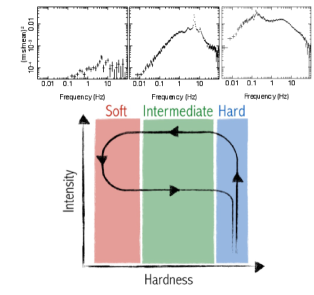
Figure 1: Bottom: Schematic demonstrating the path traced on a hardness intensity diagram (HID) for a typical (idealised) black hole binary outburst. The source passes through three broadly defined states, the hard (blue), intermediate (green) and soft (red) states. Top: Power spectra representative of these three states, with the hard and soft states on the right and left respectively. Here, the power spectra are plotted as frequency $\times$ power, such that the y-axis is in units a fractional rms variability.

The spectral transitions can be explained by the truncated disk model (Ichimaru 1977; Done et al 2007). In the hard state, the geometrically thin, optically thick accretion disk truncates at a radius larger than the innermost stable circular orbit (ISCO). The disk is therefore very weak in the spectrum and also comparatively cool. Inside of the truncation radius is a large scale height, hot accretion flow. Compton up-scattering of cool disk photons by hot electrons in this hot inner flow creates the power-law spectrum, which dominates. As the mass accretion rate increases to make the source brighter, the truncation radius moves in. This means that the inner flow is cooled by a greater luminosity of comparatively cool disk photons, leading the power-law to soften. This also naturally leads to the disk becoming more prominent in the spectrum. Alternative interpretations of the spectrum are prominent in the literature, in particular many authors suggest that the power-law spectrum originates in the base of a jet rather than an inner hot flow (Markoff, Nowak, & Wilms; Miller 2007). However, in this review I focus on the truncated disk model, which has been considered far more extensively than any other in the context of rapid X-ray variability (see e.g. Gilfanov 2010).

Variability on shorter timescales is best characterised using Fourier transforms. The power spectrum of the X-ray flux evolves just as dramatically as the X-ray spectrum during an outburst. Examples representative of each of the three states are shown at the top of Fig 1 for the source GX339-4. In the hard state there is a large amplitude of variability on a broad range of time scales, evidenced by the high normalisation and broad shape of the power spectrum (right). We can see low and high frequency breaks at $\sim 0.05$ Hz and $\sim 5$ Hz respectively where the power drops-off from ‘flat-top’ noise. As the spectrum evolves to the intermediate state, the low frequency break moves to higher frequencies and the total variability reduces (middle). The high frequency noise ($\gtrsim 10$ Hz), in contrast, stays roughly constant (Gierliński, Nikołajuk & Czerny 2008). We can also see narrow peaks in the power spectra. These are quasi-periodic oscillations (QPOs). Since they pick out a characteristic time scale in the system, they are very interesting. However, I will focus on the broad band noise here and refer the interested reader to Sara Motta’s contribution to this volume. As the spectrum continues to evolve (and the truncation radius moves further in according to the truncated disk model), the low frequency break moves to still higher frequencies and the total variability amplitude continues to reduce until, in the soft state, there is barely any variability at all (left). See e.g. van der Klis (2006) for a more detailed review.

Here, I review a paradigm that has emerged over the last $\sim 15$ years to explain the properties of the rapid aperiodic X-ray variability in the context of the truncated disk model. It is increasingly thought that this variability is due to fluctuations in the mass accretion rate. In Section 2 I review the theoretical motivation for considering propagating accretion rate fluctuations. In Section 3 I review the main observational evidence for the model and in Section 4 I discuss the remaining challenges to address in future.

2 Theoretical background

The propagation of fluctuations in an accretion flow depends on viscosity and differential rotation. As gas spirals towards the black hole, the infall velocity is likely small compared with the orbital velocity, $v_{R}<<v_{\phi}$, which is thus Keplerian to a good approximation, $v_{\phi}=\sqrt{GM/R}$. For gas at radius $R$ to drift to radius $R-dR$, it must lose angular momentum (i.e. be slowed down) through viscous shear from the differentially rotating stream of gas inside of it. The force per unit surface area (the stress) felt by the stream at $R$ is $-\eta R\Omega^{\prime}$, where $\Omega^{\prime}$ is the radial derivative of the orbital angular velocity ($\Omega=v_{\phi}/R$) and $\eta$ is the dynamic viscosity (Frank, King & Raine 2002; hereafter FKR02). The kinematic viscosity is defined as $\nu=\eta/\rho$, where $\rho$ is the gas density. This arises in a fluid through some combination of molecular transport (i.e. thermal motion of molecules in the fluid) and hydrodynamic turbulence. Accretion flows are thought to be dominated by the latter, since the former cannot generate a high enough viscosity (FKR02). We can understand the kinematic viscosity by expressing it as $\nu\sim\lambda\tilde{v}$, where $\lambda$ and $\tilde{v}$ are the characteristic size and speed of the turbulence. In the absence of a deep understanding of the physics underpinning the viscosity, Shakura & Sunyaev (1973) famously used the parameterisation, $\nu=\alpha c_{s}H$, where $c_{s}$ is the sound speed, $H$ is the height of the disk/flow and $\alpha$ is the dimensionless viscosity parameter. This comes from assuming that the turbulent motion is probably not supersonic, so $\tilde{v}\lesssim c_{s}$, and the size scale of the turbulent eddies is not larger than the disk height $\lambda\lesssim H$. This implies that $\alpha\lesssim 1$ is reasonable, although there is no a priori reason to believe that $\alpha$ is independent of radius. Over the past few decades, the magnetorotational instability (MRI: Balbus & Hawley 1991) has emerged as a strong candidate mechanism to provide the required turbulence. This is effectively tangling up of magnetic field lines in the differentially rotating gas.

The evolution of perturbations in the accretion disk can be described by the diffusion equation (Lynden-Bell & Pringle 1974). Assuming circular, Keplerian orbits and applying mass and angular momentum conservation, this takes the form

$$\frac{\partial\Sigma}{\partial t}=\frac{3}{R}\frac{\partial}{\partial R}\left\{R^{1/2}\frac{\partial}{\partial R}\left[\nu\Sigma R\right]\right\},$$ (1)

where $\Sigma=\rho H$ is the surface density. In principle, this equation is valid both for a classic geometrically thin accretion disk and also the large scale height inner hot flow thought to be present in the hard state – but only if the assumptions of Keplerian orbits and negligible vertical gradients hold. Although both of these assumptions may break down for a particularly large scale height $H/R$, they will approximately hold for reasonable parameters (e.g. Fragile et al 2007). Now let us explore the properties of the diffusion equation by introducing a $\delta$-function perturbation in the surface density at radius $R=R_{0}$ and time $t=0$. Here I explore the illustrative example set out in FKR02 using $\nu=$constant, although note that more sophisticated treatments of the viscosity are possible (Lynden-Bell & Pringle 1974; Lyubarskii 1997; Kotov et al 2001; Tanaka 2011). In this case, the surface density of an initially thin ring with mass $m$ evolves in time as

$$\Sigma(x,\tau)=\frac{m}{\pi R_{0}^{2}}\tau^{-1}x^{-1/4}\exp\left\{-\frac{(1+x^{2})}{\tau}\right\}I_{1/4}(2x/\tau),$$ (2)

where $I_{1/4}$ is a modified Bessel function and radius and time are expressed as the dimensionless variables $x=R/R_{0}$ and $\tau=12\nu tR_{0}^{-2}$. The contours and shading in Fig 2 illustrate equation 2. At time $\tau=0$, the perturbation in surface density is a narrow ring at $x=1$. With time, this ring spreads out and moves towards the black hole.

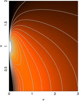
Figure 2: Representation of the Greens function from equation 2. The dimensionless time and radius variables are respectively $\tau$ and $x$. A $\delta-$function perturbation in the surface density originates at $\tau=0$, $x=1$. Lighter shades represent higher surface density, and so the perturbation initially shows up as a narrow bright patch on the plot (this saturates the colour scheme and so the perturbation appears to have finite width). The perturbation spreads out over time and moves towards smaller $x$. This is made clearer by the grey contours of constant surface density.

In a limit in which equation 1 is linear, equation 2 is a Greens function, $g(R,t)$ (with dimensionless variables replaced by physical ones). Thus, if we were to introduce fluctuations at radius $R=R_{0}$ with general form $d(t)$, the surface density will evolve in time as $\Sigma(R,t)=d(t)\ast g(R,t)$, where $\ast$ denotes a convolution. The Fourier transform of the surface density is therefore $\Sigma(R,f)=D(f)G(R,f)$. If $d(t)$ is white noise, this reduces further to $\Sigma(R,f)\propto G(R,f)$. From mass conservation, $\dot{M}(R,f)\propto\Sigma(R,f)\propto G(R,f)$ and so the Greens function tells us all we need to know about the nature of mass accretion rate fluctuations in an accretion flow.

As noted by Churazov et al (2001), we can simplify this in the limit of $R<<R_{0}$ to gain insight (i.e. taking a horizontal slice across Fig 2 at small $x$). In this case, equation 2 reduces approximately to $\Sigma\propto\tau^{5/4}\exp[-1/\tau]$. We see that a $\delta-$function spike in the surface density at $R=R_{0}$ causes a much slower rise at $R<<R_{0}$, followed by an exponential decay with a characteristic decay timescale of $\tau=1$. This characteristic timescale is called the viscous timescale and it follows from the definition of $\tau$ that

$$t_{visc}(R)=\frac{R^{2}}{12\nu}.$$ (3)

Fluctuations on timescales shorter than the viscous timescale, or in other words faster than the viscous frequency $f_{\rm visc}(R)=1/t_{\rm visc}(R)$, are therefore strongly damped by the combination of viscosity and differential rotation. The Fourier transform of a damped exponential is a zero-centred Lorentzian, and therefore the power spectrum of mass accretion rate fluctuations in the accretion disk is approximately

$$|\dot{M}(R,f)|^{2}\propto\frac{1}{1+[f/f_{\rm visc}(R)]^{2}}.$$ (4)

Note that this equation assumes that Equation 2 approximately takes the form of a damped exponential even for locally produced fluctuation (i.e. $R=R_{0}$). Considering that the very existence of the viscosity in the disk hinges on the presence of turbulence, it is fair to assume that mass accretion rate fluctuations are stirred up throughout the accretion flow by the same process that generated the viscosity. Assuming that the generated fluctuations have the nature of white noise, the power spectrum of the mass accretion rate everywhere in the accretion flow is given by equation 4 (Arevalo & Uttley 2006; Ingram & Done 2011; 2012). The viscous timescale also sets the timescale in which a perturbation is accreted. The infall velocity of accreting material is therefore $v_{R}(R)\sim Rf_{\rm visc}(R)$. This gives us the frame work of the propagating fluctuations model: perturbations propagate inwards at a speed set by viscosity and are also damped by viscosity.

So what is the viscous frequency? Using Shakura & Sunyaev’s $\alpha-$prescription one more time and setting the sound speed to $c_{s}=(H/R)v_{\phi}$ yields

$$f_{visc}(R)\approx 2\alpha(H/R)^{2}f_{\phi}(R),$$ (5)

where $f_{\phi}(R)=\Omega(R)/(2\pi)$ is the orbital frequency. From equation 5, we see that rapid variability is allowed for a large scale heigh flow, as is thought to be present in the hard state, but is damped for the thin disk (small $H/R$) present in the soft state. This is consistent with observations of the variable hard state and stable soft state (see Fig 1). We also expect the amplitude of variability generated by turbulence to increase with $H/R$ (Ingram 2012). Imagine turbulent eddies, with characteristic length scale $\sim H$, generating variability in the accretion rate. It is possible to fit $N\sim 2\pi/H$ such eddies in a ring of the accretion flow at radius $R$. If these eddies are all independent of one another and all generate variability with roughly the same mean $\mu$ and variance $\sigma^{2}$, then the entire ring will have a mean $\mu_{\rm tot}=N\mu$ and variance $\sigma^{2}_{\rm tot}=N\sigma^{2}$. The fractional rms generated by the ring is therefore $\sigma_{\rm tot}/\mu_{\rm tot}\propto(H/R)^{1/2}(\sigma/\mu)$. It is therefore expected that a thin disk will be observed to be more stable than a thick disk.

3 Observations

Many of the rapid X-ray variability properties of black hole binaries are naturally explained by the propagating mass accretion rate fluctuations model. In this Section, I cover the most prominent examples.

3.1 Power spectrum

The stable disk / variable inner flow paradigm (e.g. Revnivtsev, Gilfanov & Churazov 1999; Churazov et al 2001) predicts that the low frequency break in the power spectrum is simply set by the viscous frequency at the outer edge of the inner hot flow. This frequency increases as the truncation radius moves in during spectral evolution, naturally explaining the observed increase in the low frequency break (Wijnands & van der Klis 1999). The xspec model propfluc (Ingram & Done 2011; 2012; Ingram & van der Klis 2013) assumes a variable inner flow with some inner and outer radius, which are model parameters. The viscous frequency (or rather the surface density: the two are linked by mass conservation) as a function of $R$ is parameterised. Originally, the process of stochastic fluctuations propagating towards the black hole could only be calculated using Monte Carlo simulations. Ingram & van der Klis (2013) developed a formalism to perform exactly the same calculation analytically without making any further assumptions. propfluc additionally assumes that the QPO results from Lense-Thirring precession of the inner flow (Ingram, Done & Fragile 2009). There are now a few studies in the literature that fit the propfluc model to observed power spectra (Ingram & Done 2012; Rapisarda, Ingram & van der Klis 2014). See Stefano Rapisarda’s contribution to this volume for a more comprehensive summary of the propfluc model.

3.2 Linear RMS-flux relation

A linear RMS-flux relation was first discovered for the case of Cygnus X-1 by Uttley & McHardy (2001). Roughly speaking, this can be measured by chopping a long light curve up into short segments and calculating the mean flux for each segment and the standard deviation (absolute rms) around each of these flux measurements. Plotting the absolute rms measurements against the flux measurements, after binning in flux, reveals a striking linear relation. This relation holds for a large range of timescales – whether we use $2$s segments or $20$s segments, we still see a linear rms flux relation for Cygnus X-1. The linear rms-flux relation seems to be a ubiquitous property of variable accreting objects (Uttley 2004; Heil & Vaughan 2010; Heil, Vaughan & Uttley 2012). This property of the variability tells us that different timescales are correlated. In the picture laid out in the previous section in which different timescales are produced in different regions, the linear rms-flux relation tells us that these regions must be causally connected. Uttley, McHardy & Vaughan (2005) showed that this property rules out previously popular shot noise models, in which the variability is modelled as a sum of unrelated flares drawn from some distribution.

The propagating fluctuations model naturally predicts a linear rms-flux relation. This happens because the fluctuations produced at all radii propagate inwards. So, a fluctuation generated far from the black hole propagates inwards to modulate the faster variability produced closer to the black hole. Since this modulation is a multiplicative process, this results in intervals of low(high) flux having a low(high) variability amplitude. Fig 3 shows the an rms-flux relation calculated with propfluc. Here, I generated a long light curve ($8192$s) and split it into $2$s segments (it is still not possible to calculate the rms-flux relation predicted by the model analytically and so this plot required a Monte Carlo simulation). We see that it is indeed linear as expected.

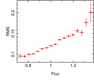
Figure 3: RMS-flux relation for a simulation using the model propfluc. The outer and inner radii of the variable hot inner flow are assumed to be $50R_{g}$ and $4.25R_{g}$ respectively. A $8192$s light curve was generated using a Monte Carlo simulation and split up into $4096$ $2$s segments. The relation is linear, consistent with observations.

3.3 Frequency-resolved spectroscopy

Another basic ingredient of the propagating fluctuations paradigm is that harder radiation is generally emitted closer to the black hole. This is simple to justify theoretically, since the gravitational energy loss experienced by accreting material increases closer to the black hole. For a thermalised accretion disk, the temperature goes as $T\propto R^{-3/4}$. For the inner flow, the outer region is cooled by a greater luminosity of comparatively cool disk photons than the inner region (which is further from the disk). We therefore expect the spectrum emitted by the inner flow to be softer at larger radius.

Revnivtsev et al (1999) used frequency-resolved spectroscopy to reinforce this picture. The frequency-resolved spectrum for the frequency range $f_{1}$ to $f_{2}$ is simply the absolute variability amplitude in this frequency range as a function of energy. Revnivtsev et al (1999) showed that the spectrum of the slow variability in Cygnus X-1 in the hard state is a hard power law, and the spectrum of the faster variability is a softer power law. This fits in nicely with the picture that the fast variability and hard radiation originate from small $R$ and the slow variability and soft radiation originate from large $R$.

3.4 Time lags

Since fluctuations take time to propagate towards the black hole, the model predicts photons emitted at small $R$ to lag photons emitted at large $R$. Since the spectrum is harder closer to the black hole, the photons emitted at small $R$ are, on average, harder than those emitted at large $R$ and therefore hard photons lag soft photons. We cannot directly observe which radius photons are emitted from, but we can isolate different Fourier frequencies. The model predicts that the time lag between hard and soft photons is longer for slow variability (low Fourier frequency) than for fast variability (high Fourier frequency). This is because slow variability can be generated anywhere in the flow but fast variability can only be generated at small $R$. Therefore, on average, fast fluctuations have not propagated as far between emitting soft and hard photons. Figure 4 shows the time lag between two broad energy bands as a function of Fourier frequency for an observation of Cygnus X-1 (black points). Here, a positive lag means that hard photons lag soft. We see that hard photons do indeed lag soft photons, and the amplitude of the lag reduces with Fourier frequency. The red line models the lag using propfluc (Ingram & van der Klis 2013 found an analytic expression for the time lags in addition to the power spectrum). The propagation time between a given pair of radii is set by the viscous frequency (since $v_{R}(R)\sim Rf_{\rm fisc}(R)$), and the radial dependence of spectral hardness is parameterised by assuming a different (power-law) radial emissivity profile for each energy band.

The time lag is also observed to depend on the energy bands considered. The greater the separation between the energy bands, the longer the lag (e.g. Kotov et al 2001). This makes intuitive sense in the propagating fluctuations picture, since the softest photons are predominantly emitted at the largest $R$ and so fluctuations from here must propagate further to reach the smallest $R$ where the hardest photons are emitted.

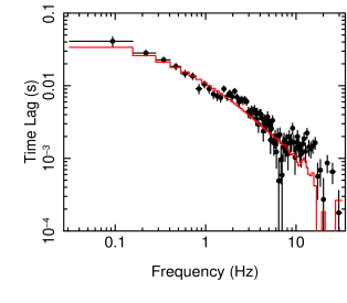
Figure 4: Time lag of the $\sim 5.6-16.6$ keV band with respect to the $\sim 2-5.6$ keV band as a function of Fourier frequency. The black points are for an RXTE observation of Cygnus X-1 (obs ID 10238-01-08-00). The red line is calculated from the model propfluc, assuming that a harder spectrum is emitted at smaller radii in the inner hot flow.

4 Discussion & Conclusions

The propagating fluctuations model can successfully explain many observational properties of black hole binaries, but there are a number of improvements that can be made and challenges to be overcome. Perhaps most obvious is the details of the observed power spectra and lag spectra. In Fig. 1, we see that the broadband noise in the observed power spectrum (presented in units of frequency $\times$ power) looks roughly like flat top noise, with high and low frequency breaks. propfluc produces exactly this shape, since it assumes that each radius of the flow generates fluctuations of the same amplitude. For some observations, however, it is clear that the broad band noise has more structure than this, with lumps and bumps often modelled as individual Lorentzian components. This structure is also in the lag spectra. Fig. 4 shows lumps in the data that are not reproduced by the model. Features tend to be present at the same frequency for both the power and lag spectra of a given observation (Grinberg et al 2014). For example, the power spectrum corresponding to the lag spectrum shown in Fig. 4 also has a hump peaking at $\sim 2-3$ Hz. It is in principle possible to reproduce these features with propfluc by simply allowing the variability generated in the flow to depend on radius. Ingram & Done (2012) demonstrated that a ‘double hump’ power spectrum can be produced by introducing enhanced variability at one particular radius (Figure 6 therein). This also impacts on the predicted lag spectrum, so even an ad hoc introduction of variability at a particular radius, creates features in the power and lag spectrum, that must be both consistent with data. In other words, a tweak that allows the model to fit the power spectrum also inevitably changes the predicted lag spectrum.

We of course should also have a good reason to introduce extra variability at a given radius. Henisey et al (2012) reported on enhanced variability at $\sim 7R_{g}$ in numerical simulations of a large scale height accretion flow caused by the misalignment of the flow spin axis with that of the black hole. The frame dragging effect (the twisting up of the surrounding spacetime by the spinning black hole) means that the black hole itself exerts a torque on the accretion flow. Fragile et al (2007) showed that this introduces ‘plunging streams’ of material at $\sim 7R_{g}$ in simulations in which the black hole spin axis is misaligned with the flow spin axis. In these plunging streams, material falls towards the black hole relatively quickly in constrast to the slow viscous drift at larger radii. Henisey et al (2012) showed that there is actually enhanced variability in the vicinity of these streams. Enhanced variability could alternatively / additionally come from the disk. When the standard picture was of stable disk and variable inner flow, Wilkinson & Uttley (2009) found that the disk was actually variable on timescales $\gtrsim 1$s in hard state observations of GX339-4 and SWIFT J1753.5−0127. Therefore, bumps in the power spectra at low frequency could potentially come from variability in the disk rather than the flow (see Stefano Rapisarda’s contribution to this volume). This makes a prediction in terms of the lag spectrum, since fluctuations from the disk take time to propagate to the hard emitting region, which can be tested directly against data (Rapisarda et al in prep).

A significant improvement to the model would be to use a more sophisticated Green’s function to model the damping and propagation of fluctuations, rather than using the current Lorentzian treatment (i.e. equation 4) with propagation occurring at the viscous infall speed. It is relatively easy to make this change if the model calculation uses a Monte Carlo simulation. It is, however, far more difficult to adapt the analytic formalism of Ingram & van der Klis (2013) for the case of a general Greens function, which is required for the model to realistically be tested against data.

Another important physical effect that has not been mentioned thus far is reflection of hard X-ray photons from the outer disk. Reflected photons contribute a relatively small fraction of the observed flux for most observations of black hole binaries but certainly not a negligible fraction. Also, reflection provides a powerfull diagnostic of the accretion flow, since the narrow iron line emitted due to reflection is distorted in a characteristic way by the orbital motion of disk material. This effect was considered in the context of propagating mass accretion rate fluctuations by Kotov et al (2001) and should also be included in future versions of the propfluc model.

In conclusion, the general propagating fluctuations picture is very well motivated theoretically and the data provide strong evidence to back this up. In particular the rms-flux relation is a natural consequence of propagating fluctuations but very difficult to contrive in alternative scenarios. The details of the model, however, are still uncertain. Systematic, quantitative testing of increasingly sophisticated versions of the model against the huge archive of public data provided by RXTE will address this going forward.