Optimizing Solution Quality in Synchronization Synthesis

Abstract

Given a multithreaded program written assuming a friendly, non-preemptive scheduler, the goal of synchronization synthesis is to automatically insert synchronization primitives to ensure that the modified program behaves correctly, even with a preemptive scheduler. In this work, we focus on the quality of the synthesized solution: we aim to infer synchronization placements that not only ensure correctness, but also meet some quantitative objectives such as optimal program performance on a given computing platform.

The key step that enables solution optimization is the construction of a set of global constraints over synchronization placements such that each model of the constraints set corresponds to a correctness-ensuring synchronization placement. We extract the global constraints from generalizations of counterexample traces and the control-flow graph of the program. The global constraints enable us to choose from among the encoded synchronization solutions using an objective function. We consider two types of objective functions: ones that are solely dependent on the program (e.g., minimizing the size of critical sections) and ones that are also dependent on the computing platform. For the latter, given a program and a computing platform, we construct a performance model based on measuring average contention for critical sections and the average time taken to acquire and release a lock under a given average contention.

We empirically evaluated that our approach scales to typical module sizes of many real world concurrent programs such as device drivers and multithreaded servers, and that the performance predictions match reality. To the best of our knowledge, this is the first comprehensive approach for optimizing the placement of synthesized synchronization.

1 Introduction

Synchronization synthesis aims to enable programmers to concentrate on the functionality of the program, and not on the low-level synchronization. One of the main challenges in synchronization synthesis, and in program synthesis in general, is to produce a solution that not only satisfies the specification, but also is good (if not optimal) according to various metrics such as performance and conformance to good programming practices. Optimizing for performance for a given architecture is a challenging problem, but it is an area where program synthesis can have an advantage over the traditional approach to program development: the fact that synthesis takes a high-level specification as input gives the synthesizer a lot of freedom to find a solution that is both correct and performs well.

Optimization is hard for the common approach to synchronization synthesis, which implements a counterexample-guided inductive synthesis (CEGIS) loop. A counterexample is given by a trace, and typically, this trace is immediately (greedily) removed from the program by placing synchronization. The advantage of this trace-based approach is that traces are computationally easier to analyze. However, the greedy approach makes it difficult to optimize the final solution with respect to qualities such as performance.

We propose a new approach that keeps the trace-based technique, but uses it to collect a set of global constraints over synchronization placements. Each model of the global constraints corresponds to a correct synchronization placement. Constructing the global constraints is a key step in our approach, as they enable us to choose from among the encoded synchronization solutions using an objective function.

The global constraints are obtained by analyzing the program with respect to the concurrency specification. In this paper, we focus solely on one type of synchronization – locks. Our concurrency specification consists of three parts: preemption-safety, deadlock-freedom, and a set of standard locking discipline conditions. The goal of preemption-safety (proposed in CAV15 ) is to enable the programmer to program assuming a friendly, non-preemptive scheduler. It is then the task of the synthesizer to ensure that every execution under the preemptive scheduler is observationally equivalent to an execution under the preemptive scheduler. Two program executions are observationally equivalent if they generate the same sequences of calls to interfaces of interest. We consider a program correct if, in addition to preemption-safety, it does not produce deadlocks, and if it follows good programming practices with respect to locks: we require no double locking, no double unlocking and several other conditions that we refer to as legitimate locking. Legitimate locking helps making the final solution readable and maintainable. The salient point of our correctness notion is that it is generic — the programmer does not need to write a specification for each application separately.

The global constraints resulting from the preemption-safety requirement are obtained from an analysis of generalized counterexamples. The analysis uses the CEGIS approach of CAV15 , where the key steps in checking preemption-safety are a coarse, data-oblivious abstraction (shown to work well for systems code), and an algorithm for bounded language inclusion checking. The approach of CAV15 is greedy, that is, it immediately places locks to eliminate the counterexample. In contrast, we do not place locks, but instead infer mutual exclusion (mutex) constraints for eliminating the counterexample. We then enforce these mutex constraints in the language inclusion check to avoid getting the same counterexample again. We accumulate the mutex constraints from all counterexamples iteratively generated by the language inclusion check. Once the language inclusion check succeeds, we construct the set of global constraints using the accumulated mutex constraints and constraints for enforcing deadlock-freedom and legitimate locking.

Given the global constraints, we can choose from among the encoded solutions using an objective function. We consider two types of objective functions: ones that are solely dependent on the program and ones that are also dependent on the computing platform and workload. Examples of objective functions of the first type include minimizing the number of lock statements (leading to coarse-grained locking) and maximizing concurrency (leading to fine-grained locking). We encode such an objective function, together with the global constraints, into a weighted MaxSAT problem, which is then solved using an off-the-shelf solver.

In order to choose a lock placement (from among the ones encoded by global constraints) that has a good performance, we use an objective function that depends on a particular machine architecture and workload. The objective function is given by a performance model. We emphasize that the model is based on measuring parameters of a particular architecture running the program. In particular, it is based on measuring the average time taken to acquire and release a lock under a given level of contention (this part depends only on the architecture) and the average time it takes to execute the critical section, and the average contention for critical sections (this part depends on the architecture, the program, and the workload). The optimization procedure using the performance model and the global constraints works as follows. First, we parameterize the space of solutions by the sizes of critical sections and the number of locks taken. Second, we find the parameter values that maximize performance. Third, we find a solution of the global constraints closest to the parameter values that yield maximal performance.

We empirically evaluate that our approach scales to typical module sizes of many real world concurrent programs such as device drivers and multithreaded servers ($\sim$1000 LOC). We use our synthesis tool (with architecture-independent objective functions) on a number of device driver benchmarks and find that the synthesis times are comparable to an existing tool CAV15 that implements a standard CEGIS-based algorithm; we emphasize that our tool finds an optimal lock placement that guarantees preemption-safety, deadlock freedom and legitimate locking. Furthermore, we evaluate the tool with an objective function given by our performance model. We use the memcached network server that provides an in-memory key-value store, specifically the module used by server worker threads to access the store. We found that the performance model predictions match reality, and that we obtained different locking schemes based on the values of parameters of the performance model.

static void* worker_thread(void *arg) {
    for (j = 0; j < niter; j++) {
        sharedX();
        sharedY();
        local();
        sharedZ();
}  };

Figure 1: Example: Work sharing

The contributions of this work are:

• To the best of our knowledge, this is the first comprehensive approach for finding and optimizing lock placement. The approach is comprehensive, as it fully solves the lock placement problem on realistic (albeit simplified) systems code.

• We use trace analysis to obtain global constraints each of whose solutions gives a legitimate lock placement, thus enabling choosing from among the encoded correct solutions using an objective function.

• A method for lock placement for machine-independent objective functions, based on weighted MaxSAT solving.

• Optimization of lock placement using a performance model obtained by measurement and profiling on a given platform.

1.1 Related Work

Synthesis of lock placement is an active research area bloem ; VYY10 ; CCG08 ; EFJM07 ; UBES10 ; DR98 ; VTD06 ; ramalingam ; SLJB08 ; ZSZSG08 ; shanlu ; CAV11 ; CAV13 ; CAV14 ; CAV15 ; POPL15 . There are works that optimize lock placement: for instance the paper by Emmi et al. EFJM07 , Cherem et al. CCG08 , and Zhang et al. ZSZSG08 . These papers takes as an input a program annotated with atomic sections, and replace them with locks, using several types of fixed objective functions. In contrast, our work does not need the annotations with atomic sections, and does not optimize using a fixed objective function, but rather using a performance model obtained by performing measurements on a particular architecture.

Another approach is to not require the programmer to annotate the program with atomic sections, but rather infer them or infer locks directly VYY10 ; bloem ; DR98 ; CAV13 ; CAV14 ; CAV15 ; POPL15 . All these works also either do not optimize the lock placement, or do so for a fixed objective function, not for a given architecture. The work CAV11 proposes concurrency synthesis w.r.t. a performance model, but it does not produce such models for a given machine architecture.

Jin et a shanlu describe a tool CFix that can detect and fix concurrency bugs by identifying bug patterns in the code. CFix also simplifies its own patches by merging fixes for related bugs.

Usui et al. UBES10 provide a dynamic adaptive lock placement algorithm, which can be precise but necessitates runtime overhead.

Our abstraction is based on the one from CAV15 , which is similar to abstractions that track reads and writes to individual locations (e.g., VYRS10 ; AKNP14 ). In VYY10 the authors rely on assertions for synchronization synthesis and include iterative abstraction refinement in their framework, which could be integrated in our approach.

1.2 Illustrative Example

One of the main contributions of the paper is a synthesis approach that allows optimization for a particular computing platform and program. We will demonstrate on an example that varying parameters of our performance model, which corresponds to varying the machine architecture and usage pattern (contention), can lead to a different solution with best performance.

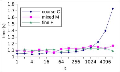
Figure 2: Performance under various locking schemes

Consider the function worker_thread in Figure 1 that is called by a number of worker threads in a work-sharing setting. The worker_thread function calls three functions that access shared memory: sharedX(), sharedY(), and sharedZ(). Each of the three functions needs to be called mutually exclusively with itself, but it does not conflict with the other two functions. None of the three functions uses locks internally. The function local() does not access shared memory. If we consider locking schemes that use only one lock, and lock only within an iteration of the loop, then there are a number of correct locking schemes. First, there is a coarse-grained version $C$ which locks before the call to sharedX() and unlocks after the call to sharedZ(). Second, there is a fine-grained version $F$ that locks each function separately. Third, there are intermediate versions, such as a version $M$ that locks before the call to sharedX(), unlocks before the call to local(), and then it locks again the call to sharedZ().

Clearly, which of the correct versions will have the best performance depends on the program, the contention, and the architecture. For instance, with very low contention, the coarse-grained version would be fastest. On the other hand, with contention, and if local() is expensive enough, the third version performs best, as it releases the lock before calling local().

We further demonstrate with a small experiment (Figure 2) that often no locking scheme is uniformly better. We considered variants of the program in Figure 1 which differ in how long it takes to execute the function local() (parameter lt in Figure 2). We kept the other parameters (such as contention and number of threads) constant (there were $4$ threads). We see that if the call to local is cheap, then the coarse-grained version performs better, but it can be perform very badly otherwise. The other two versions $M$ and $F$ perform comparably.

The example is similar to our main case study of the memcached server. We demonstrate on that case study that the performance model helps us choose the option with the best performance, and that it does not have to be the most coarse-grained or the most fine-grained locking solution.

2 Formal Framework

We present the syntax and semantics of a concrete concurrent while language $\mathcal{W}$, followed by the syntax and semantics of an abstract concurrent while language ${\mathcal{W}}_{abs}$. While $\mathcal{W}$ (and our tool) permits function call and return statements, we skip these constructs in the formalization below. We conclude the section by formalizing our notion of correctness for concrete concurrent programs.

In our work, we assume a read or a write to a single shared variable executes atomically and further assume a sequentially consistent memory model.

2.1 Concurrent Programs

Syntax of $\mathcal{W}$ (Fig. 3). A concurrent program $\mathcal{C}$ is a finite collection of threads $\langle\mathtt{T}_{1},\ldots,\mathtt{T}_{n}\rangle$ where each thread is a statement written in the syntax of $\mathcal{W}$. All $\mathcal{W}$ variables (shared program variables s_var, local program variables l_var, lock variables lk_var, condition variables c_var and guard variables g_var) range over integers. Each statement is labeled with a unique location identifier ${\tt loc}$; we denote by $\mathtt{stmt}({{\tt loc}})$ the statement labeled by ${\tt loc}$.

The language $\mathcal{W}$ includes standard syntactic constructs such as assignment, conditional, loop, synchronization, goto and yield statements. In $\mathcal{W}$, we only permit expressions that read from at most one shared variable and assignments that either read from or write to exactly one shared variable. The language also includes assume, assume_not, set and unset statements whose use will be clarified later. Most significantly, $\mathcal{W}$ permits reading from ($\mathtt{in}(\sf tag)$) and writing to ($\mathtt{out}(\sf tag,s\_expr)$) a communication channel tag between the program and an interface to an external system. In practice, we use the tags to model device registers. In our presentation, we consider only a single external interface.

    

l_expr::= constant | * | l_var |
          operator(l_expr, l_expr, ... , l_expr)
s_expr::= s_var |
          operator(s_var, l_expr, ..., l_expr)
lstmt ::= loc: stmt | lstmt; lstmt
stmt  ::= s_var := l_expr | l_var := s_expr |
          s_var := havoc() | while (s_expr) lstmt |
          if (s_expr) lstmt else lstmt |
          s_var := in(tag) | out(tag,s_expr) |
          lock(lk_var)  | unlock(lk_var) |
          wait(c_var) | wait_not(c_var) |
          notify(c_var) | reset(c_var)
          assume(g_var) | assume_not(g_var) |
          set(g_var) | unset(g_var) |
          goto loc | yield | skip

    

Figure 3: Syntax of $\mathcal{W}$

Semantics of $\mathcal{W}$. We first define the semantics of a single thread in $\mathcal{W}$, and then extend the definition to concurrent non-preemptive and preemptive semantics.

Single-thread semantics (Fig. 4). Let us fix a thread identifier $\mathit{tid}$. We use $\mathit{tid}$ interchangeably with the program it represents. A state of a single thread is given by $\langle\mathcal{V},\ell\rangle$ where $\mathcal{V}$ is a valuation of all program variables visible to thread $\mathit{tid}$, and $\ell$ is a location identifier, indicating the statement in $\mathit{tid}$ to be executed next.

We define the flow graph $\cal G_{\mathit{tid}}$ for thread $\mathit{tid}$ in a manner similar to the control-flow graph of $\mathit{tid}$. Each node of $\cal G_{\mathit{tid}}$ is labeled with a unique labeled statement of $\mathit{tid}$ (unlike a control-flow graph, statements in the same basic block are not merged into a single node). The edges of $\cal G_{\mathit{tid}}$ capture the flow of control in $\mathit{tid}$. Nodes labeled with $\mathtt{if(s\_expr)}$ and $\mathtt{while(s\_expr)}$ statements have two outgoing edges, labeled with $\mathtt{assume\;s\_expr}$ and $\mathtt{assume\;\neg s\_expr}$, respectively. The flow graph $\cal G_{\mathit{tid}}$ has a unique entry node and a unique exit node. The entry node is the first labeled statement in $\mathit{tid}$; we denote its location identifier by $\mathtt{first}_{\mathit{tid}}$. The exit node is a special node corresponding to a hypothetical statement $\mathtt{last}_{\mathit{tid}}:\,\mathtt{skip}$ placed at the end of $\mathit{tid}$.

We define successors of locations of $\mathit{tid}$ using $\cal G_{\mathit{tid}}$. The location last has no successors. We define $\mathtt{succ}(\ell)=\ell^{\prime}$ if node $\ell:\mathtt{stmt}$ in $\cal G_{\mathit{tid}}$ has exactly one outgoing edge to node $\ell^{\prime}:\mathtt{stmt}^{\prime}$. We define $\mathtt{succ}_{1}(\ell)=\ell_{1}$ and $\mathtt{succ}_{2}(\ell)=\ell_{2}$ if node $\ell:\mathtt{stmt}$ in $\cal G_{\mathit{tid}}$ has exactly two outgoing edges to nodes $\ell_{1}:\mathtt{stmt}_{1}$ and $\ell_{2}:\mathtt{stmt}_{2}$.

We can now define the single-thread operational semantics. A single execution step $\langle\mathcal{V},\ell\rangle\xrightarrow{\alpha}\langle\mathcal{V}^{\prime},\ell^{\prime}\rangle$ changes the program state from $\langle\mathcal{V},\ell\rangle$ to $\langle\mathcal{V}^{\prime},\ell^{\prime}\rangle$, while optionally outputting an observable symbol $\alpha$. The absence of a symbol is denoted using $\epsilon$. In the following, $e$ represents an expression and $e[v/\mathcal{V}[v]]$ evaluates an expression by replacing all variables $v$ with their values in $\mathcal{V}$.

In Fig. 4, we present a partial set of rules for single execution steps. The only rules which involve output of an observable are:

1. Havoc: Statement $\ell:v:={\tt havoc}$ assigns $v$ a non-deterministic value (say $k$) and outputs the observable $(\mathit{tid},{\tt havoc},k,v)$.

2. Input, Output: $\ell:x:=\mathtt{in}(t)$ and $\ell:\mathtt{out}(t,e)$ read and write values to the channel $t$, and output $(\mathit{tid},\mathtt{in},k,t)$ and $(\mathit{tid},\mathtt{out},k,t)$, where $k$ is the value read or written, respectively.

Intuitively, the observables record the sequence of non-deterministic guesses, as well as the input/output interaction with the tagged channels. The semantics of the synchronization statements shown in Fig. 4 is standard.

The semantics of assume, assume_not, set and unset statements are identical to that of wait, wait_not, notify and reset statements, respectively. Thus, $\mathtt{assume}(g)$ and $\mathtt{assume\_not}(g)$ execute iff guard variable $g$ equals $1$ and $0$, respectively. Statements $\mathtt{set}(g)$ and $\mathtt{unset}(g)$ assign $1$ and $0$ to guard variable $g$, respectively.

Figure 4: A partial set of rules for single-thread semantics of $\mathcal{W}$

    $\begin{array}[b]{@{}l@{}}\begin{array}[]{@{}c@{}}\mathtt{stmt}({\ell})=v:={\tt havoc}\qquad k\in\mathbb{N}\qquad\ell^{\prime}=\mathtt{succ}(\ell)\\ \hline\cr\raisebox{0.0pt}[10.76385pt]{}\langle\mathcal{V},\ell\rangle\xrightarrow{(\mathit{tid},{\tt havoc},k,x)}\langle\mathcal{V}[x:=k],\ell^{\prime}\rangle\end{array}\mbox{{\sc Havoc} }\\ \end{array}$
$\begin{array}[b]{@{}l@{}}\begin{array}[]{@{}c@{}}\mathtt{stmt}({\ell})=v:=\mathtt{in}(t)\qquad k\in\mathbb{N}\qquad\ell^{\prime}=\mathtt{succ}(\ell)\\ \hline\cr\raisebox{0.0pt}[10.76385pt]{}\langle\mathcal{V},\ell\rangle\xrightarrow{(\mathit{tid},{\tt in},k,t)}\langle\mathcal{V}[x:=k],\ell^{\prime}\rangle\end{array}\mbox{{\sc Input} }\\ \end{array}$
$\begin{array}[b]{@{}l@{}}\begin{array}[]{@{}c@{}}\mathtt{stmt}({\ell})=\mathtt{out}(t,e)\quad e[v/\mathcal{V}[v]]=k\quad\ell^{\prime}=\mathtt{succ}(\ell)\\ \hline\cr\raisebox{0.0pt}[10.76385pt]{}\langle\mathcal{V},\ell\rangle\xrightarrow{(\mathit{tid},{\tt\mathcal{O}},k,t)}\langle\mathcal{V},\ell^{\prime}\rangle\end{array}\mbox{{\sc Output} }\\ \end{array}$
$\begin{array}[b]{@{}l@{}}\begin{array}[]{@{}c@{}}\mathtt{stmt}({\ell})=\mathtt{lock}(lk)\qquad\mathcal{V}[lk]=0\qquad\ell^{\prime}=\mathtt{succ}(\ell)\\ \hline\cr\raisebox{0.0pt}[10.76385pt]{}\langle\mathcal{V},\ell\rangle\xrightarrow{\epsilon}\langle\mathcal{V}[lk:=\mathit{tid}],\ell^{\prime}\rangle\end{array}\mbox{{\sc Lock} }\\ \end{array}$
$\begin{array}[b]{@{}l@{}}\begin{array}[]{@{}c@{}}\mathtt{stmt}({\ell})=\mathtt{unlock}(lk)\qquad\mathcal{V}[lk]=\mathit{tid}\qquad\ell^{\prime}=\mathtt{succ}(\ell)\\ \hline\cr\raisebox{0.0pt}[10.76385pt]{}\langle\mathcal{V},\ell\rangle\xrightarrow{\epsilon}\langle\mathcal{V}[lk:=\mathit{tid}],\ell^{\prime}\rangle\end{array}\mbox{{\sc Unlock} }\\ \end{array}$
$\begin{array}[b]{@{}l@{}}\begin{array}[]{@{}c@{}}\mathtt{stmt}({\ell})=\mathtt{wait}(cv)\qquad\mathcal{V}[cv]=1\qquad\ell^{\prime}=\mathtt{succ}(\ell)\\ \hline\cr\raisebox{0.0pt}[10.76385pt]{}\langle\mathcal{V},\ell\rangle\xrightarrow{\epsilon}\langle\mathcal{V},\ell^{\prime}\rangle\end{array}\mbox{{\sc Wait} }\\ \end{array}$
$\begin{array}[b]{@{}l@{}}\begin{array}[]{@{}c@{}}\mathtt{stmt}({\ell})=\mathtt{wait\_not}(cv)\quad\mathcal{V}[cv]=0\quad\ell^{\prime}=\mathtt{succ}(\ell)\\ \hline\cr\raisebox{0.0pt}[10.76385pt]{}\langle\mathcal{V},\ell\rangle\xrightarrow{\epsilon}\langle\mathcal{V},\ell^{\prime}\rangle\end{array}\mbox{{\sc Wait\_not} }\\ \end{array}$
$\begin{array}[b]{@{}l@{}}\begin{array}[]{@{}c@{}}\mathtt{stmt}({\ell})=\mathtt{notify}(cv)/\mathtt{reset}(cv)\qquad\ell^{\prime}=\mathtt{succ}(\ell)\\ \hline\cr\raisebox{0.0pt}[10.76385pt]{}\langle\mathcal{V},\ell\rangle\xrightarrow{\epsilon}\langle\mathcal{V}[cv:=1/0],\ell^{\prime}\rangle\end{array}\mbox{{\sc Notify/Reset} }\\ \end{array}$
    

Concurrent semantics. A state of a concurrent program is given by $\langle\mathcal{V},ctid,(\ell_{1},\ldots,\ell_{n})\rangle$ where $\mathcal{V}$ is a valuation of all program variables, $ctid$ is the thread identifier of the currently executing thread and $\ell_{1},\ldots,\ell_{n}$ are the locations of the statements to be executed next in threads $\mathtt{T}_{1}$ to $\mathtt{T}_{n}$, respectively. Initially, all program variables and $ctid$ equal $0$ and for each $i\in[1,n]:\ell_{i}=\mathtt{first}_{i}$.

Figure 5: Non-preemptive semantics

$\begin{array}[b]{@{}l@{}}\begin{array}[]{@{}c@{}}ctid=i\qquad\langle\mathcal{V},\ell_{i}\rangle\xrightarrow{\alpha}\langle\mathcal{V}^{\prime},\ell_{i}^{\prime}\rangle\\ \hline\cr\raisebox{0.0pt}[10.76385pt]{}\langle\mathcal{V},ctid,(\ldots,\ell_{i},\ldots)\rangle\xrightarrow{\alpha}\langle\mathcal{V},ctid,(\ldots,\ell_{i}^{\prime},\ldots)\rangle\end{array}\mbox{{\sc Seq} }\\ \end{array}$

$\begin{array}[b]{@{}l@{}}\begin{array}[]{@{}c@{}}ctid=i\quad\ell_{i}=\mathtt{last}_{i}\quad ctid^{\prime}\in\{1,\ldots,n\}\setminus\{i\}\\ \hline\cr\raisebox{0.0pt}[10.76385pt]{}\langle\mathcal{V},ctid,(\ldots,\ell_{i},\ldots)\rangle\xrightarrow{\epsilon}\langle\mathcal{V},ctid^{\prime},(\ldots,\ell_{i},\ldots)\rangle\end{array}\mbox{{\sc Thread\_end} }\\ \end{array}$

$\begin{array}[b]{@{}l@{}}\begin{array}[]{@{}c@{}}\mathtt{stmt}({\ell_{i}})=\mathtt{lock}(lk)/\mathtt{wait}(cv)/\mathtt{wait\_not}(cv)/\mathtt{yield}\\[4.30554pt] ctid=i\qquad ctid^{\prime}\in\{1,\ldots,n\}\qquad\ell_{i}^{\prime}=\mathtt{succ}(\ell)\\ \hline\cr\raisebox{0.0pt}[10.76385pt]{}\langle\mathcal{V},ctid,(\ldots,\ell_{i},\ldots)\rangle\xrightarrow{\epsilon}\langle\mathcal{V},ctid^{\prime},(\ldots,\ell_{i}^{\prime},\ldots)\rangle\end{array}\mbox{{\sc Nswitch} }\\ \end{array}$

Figure 6: Additional rule for preemptive semantics

$\begin{array}[b]{@{}l@{}}\begin{array}[]{@{}c@{}}ctid^{\prime}\in\{1,\ldots,n\}\\ \hline\cr\raisebox{0.0pt}[10.76385pt]{}\langle\mathcal{V},ctid,(\ell_{1},\ldots,\ell_{n})\rangle\xrightarrow{\epsilon}\langle\mathcal{V},ctid^{\prime},(\ell_{1},\ldots,\ell_{n})\rangle\end{array}\mbox{{\sc Pswitch} }\\ \end{array}$

Non-preemptive semantics (Fig. 5). The non-preemptive semantics ensures that a single thread from the program keeps executing using the single-thread semantics (Rule Seq) until one of the following occurs: (a) the thread finishes execution (Rule Thread_end) or it encounters a (b) yield, lock, wait or wait_not statement (Rule Nswitch). In these cases, a context-switch is possible.

Preemptive semantics (Fig. 5, Fig. 6). The preemptive semantics of a program is obtained from the non-preemptive semantics by relaxing the condition on context-switches, and allowing context-switches at all program points. In particular, the preemptive semantics consist of the rules of the non-preemptive semantics and the single rule Pswitch in Fig. 6.

void open_dev() {
1: while (*) {
2:   if (open==0)
3:      power_up();
4:   open:=open+1;
5: yield; } }

      

void open_dev_abs() {
1: while (*) {
2: r(open);
   if (*)
3:    w(dev);
4: r(open);
   w(open);
5: yield; } }

Figure 7: Example procedure and its abstraction

2.2 Abstract Concurrent Programs

For concurrent programs written in $\mathcal{W}$ communicating with external system interfaces, it suffices to focus on a simple, data-oblivious abstraction (CAV15 ). The abstraction tracks types of accesses (read or write) to each memory location while abstracting away their values. Inputs/outputs to an external interface are modeled as writes to a special memory location (dev). Havocs become ordinary writes to the variable they are assigned to. Every branch is taken non-deterministically and tracked. Given $\mathcal{C}$ written in $\mathcal{W}$, we denote by $\mathcal{C}_{abs}$ the corresponding abstract program written in ${\mathcal{W}}_{abs}$.

Example. We present a procedure open_dev() and its abstraction in Fig. 7. The function power_up() represents a call to a device.

Abstract Syntax (Fig. 8). In the figure, var denotes all shared program variables and the dev variable. Observe that the abstraction respects the valuations of the lock, condition and guard variables.

    

lstmt ::= loc: stmt | lstmt; lstmt
stmt  ::= r(var) | w(var) | if(*) lstmt else lstmt
          | while(*) lstmt |
          lock(lk_var)  | unlock(lk_var) |
          wait(c_var) | wait_not(c_var) |
          notify(c_var) | reset(c_var) |
          assume(g_var) | assume_not(g_var) |
          set(g_var) | unset(g_var) |
          goto loc | yield | skip

    

Figure 8: Syntax of ${\mathcal{W}}_{abs}$

Abstract Semantics. As before, we first define the semantics of ${\mathcal{W}}_{abs}$ for a single-thread.

Single-thread semantics (Fig. 9.) The abstract state of a single thread $\mathit{tid}$ is given simply by $\langle\ell\rangle$ where $\ell$ is the location of the statement in $\mathit{tid}$ to be executed next. We define the flow graph and successors for locations in the abstract program $\mathit{tid}$ in the same way as before. An abstract observable symbol is of the form: $(\mathit{tid},\theta,\ell)$, where $\theta\in\{\mathtt{(read,v),(write,v),if,else,loop,exitloop}\}$. The symbol $\theta$ records the type of access to variables along with the variable name $(\mathtt{(read,v),(write,v)})$ and records non-deterministic branching choices $\{\mathtt{if,else,loop,exitloop}\}$. Fig. 9 presents the rules for statements unique to ${\mathcal{W}}_{abs}$; the rules for statements common to ${\mathcal{W}}_{abs}$ and $\mathcal{W}$ are the same.

Figure 9: Partial set of rules for single-thread semantics of ${\mathcal{W}}_{abs}$

$\begin{array}[b]{@{}l@{}}\begin{array}[]{@{}c@{}}\mathtt{stmt}({\ell})=\mathtt{r}(v)\qquad\ell^{\prime}=\mathtt{succ}(\ell)\\ \hline\cr\raisebox{0.0pt}[10.76385pt]{}\langle\ell\rangle\xrightarrow{(\mathit{tid},(\mathtt{read},v),\ell)}\langle\ell^{\prime}\rangle\end{array}\mbox{{\sc Read} }\\ \end{array}$

$\begin{array}[b]{@{}l@{}}\begin{array}[]{@{}c@{}}\mathtt{stmt}({\ell})=\mathtt{w}(v)\qquad\ell^{\prime}=\mathtt{succ}(\ell)\\ \hline\cr\raisebox{0.0pt}[10.76385pt]{}\langle\ell\rangle\xrightarrow{(\mathit{tid},(\mathtt{write},v),\ell)}\langle\ell^{\prime}\rangle\end{array}\mbox{{\sc Write} }\\ \end{array}$

$\begin{array}[b]{@{}l@{}}\begin{array}[]{@{}c@{}}\mathtt{stmt}({\ell})=\mathtt{if}(*)\;s_{1}\;\mathtt{else}\;s_{2}\qquad\ell^{\prime}=\mathtt{succ}_{1}(\ell)\\ \hline\cr\raisebox{0.0pt}[10.76385pt]{}\langle\ell\rangle\xrightarrow{(\mathit{tid},\mathtt{if},\ell)}\langle\ell^{\prime}\rangle\end{array}\mbox{{\sc If1} }\\ \end{array}$

$\begin{array}[b]{@{}l@{}}\begin{array}[]{@{}c@{}}\mathtt{stmt}({\ell})=\mathtt{if}(*)\;s_{1}\;\mathtt{else}\;s_{2}\qquad\ell^{\prime}=\mathtt{succ}_{2}(\ell)\\ \hline\cr\raisebox{0.0pt}[10.76385pt]{}\langle\ell\rangle\xrightarrow{(\mathit{tid},\mathtt{else},\ell)}\langle\ell^{\prime}\rangle\end{array}\mbox{{\sc If2} }\\ \end{array}$

$\begin{array}[b]{@{}l@{}}\begin{array}[]{@{}c@{}}\mathtt{stmt}({\ell})=\mathtt{while}(*)\;s\qquad\ell^{\prime}=\mathtt{succ}_{1}(\ell)\\ \hline\cr\raisebox{0.0pt}[10.76385pt]{}\langle\ell\rangle\xrightarrow{(\mathit{tid},\mathtt{loop},\ell)}\langle\ell^{\prime}\rangle\end{array}\mbox{{\sc While1} }\\ \end{array}$

$\begin{array}[b]{@{}l@{}}\begin{array}[]{@{}c@{}}\mathtt{stmt}({\ell})=\mathtt{while}(*)\;s\qquad\ell^{\prime}=\mathtt{succ}_{2}(\ell)\\ \hline\cr\raisebox{0.0pt}[10.76385pt]{}\langle\ell\rangle\xrightarrow{(\mathit{tid},\mathtt{exitloop},\ell)}\langle\ell^{\prime}\rangle\end{array}\mbox{{\sc While2} }\\ \end{array}$

Concurrent semantics. A state of an abstract concurrent program is given by $\langle\mathcal{V}_{o},ctid,(\ell_{1},\ldots,\ell_{n})\rangle$ where $\mathcal{V}_{o}$ is a valuation of all lock, condition and guard variables, $ctid$ is the current thread identifier and $\ell_{1},\ldots,\ell_{n}$ are the locations of the statements to be executed next in threads $\mathtt{T}_{1}$ to $\mathtt{T}_{n}$, respectively. The non-preemptive and preemptive semantics of a concurrent program written in ${\mathcal{W}}_{abs}$ are defined in the same way as that of a concurrent program written in $\mathcal{W}$.

2.3 Executions and Observable Behaviours

Let $\mathbb{W}$, $\mathbb{W}_{abs}$ denote the set of all concurrent programs in $\mathcal{W}$, ${\mathcal{W}}_{abs}$, respectively.

Executions. A non-preemptive/preemptive execution of a concurrent program $\mathcal{C}$ in $\mathbb{W}$ is an alternating sequence of program states and (possibly empty) observable symbols, $s_{0}\alpha_{1}s_{1}\ldots\alpha_{k}s_{k}$, such that (a) $s_{0}$ is the initial state of $\mathcal{C}$ and (b) $\forall j\in[0,k-1]$, according to the non-preemptive/preemptive semantics of $\mathcal{W}$, we have $s_{j}\xrightarrow{\alpha_{j+1}}{s_{j+1}}$. A non-preemptive/preemptive execution of a concurrent program $\mathcal{C}_{abs}$ in $\mathbb{W}_{abs}$ is defined in the same way, replacing the corresponding semantics of $\mathcal{W}$ with that of ${\mathcal{W}}_{abs}$.

Given an execution $\pi$, let $\mathsf{obs}(\pi)$ denote the sequence of non-empty observable symbols in $\pi$.

Observable Behaviours. The non-preemptive/preemptive observable behaviour of program $\mathcal{C}$ in $\mathbb{W}$, denoted $[\![\mathcal{C}]\!]^{NP}$/$[\![\mathcal{C}]\!]^{P}$, is the set of all sequences $\omega$ of non-empty observable symbols such that $\omega=\mathsf{obs}(\pi)$ for some non-preemptive/preemptive execution $\pi$ of $\mathcal{C}$. The non-preemptive/preemptive observable behaviour of program $\mathcal{C}_{abs}$ in $\mathbb{W}_{abs}$, denoted $[\![\mathcal{C}_{abs}]\!]^{NP}$/$[\![\mathcal{C}_{abs}]\!]^{P}$, is defined similarly.

2.4 Program Correctness

We specify correctness of concurrent programs in $\mathbb{W}$ using three implicit criteria, presented below.

Preemption-safety. Observable behaviours $\omega_{1}$ and $\omega_{2}$ of a program $\mathcal{C}$ in $\mathbb{W}$ are equivalent if: (a) the subsequences of $\omega_{1}$ and $\omega_{2}$ containing only symbols of the form $(\mathit{tid},\mathtt{in},k,t)$ and $(\mathit{tid},\mathtt{out},k,t)$ are equal and (b) for each thread identifier $\mathit{tid}$, the subsequences of $\omega_{1}$ and $\omega_{2}$ containing only symbols of the form $(\mathit{tid},\mathtt{havoc},k,x)$ are equal. Intuitively, observable behaviours are equivalent if they have the same interaction with the interface, and the same non-deterministic choices in each thread. For sets $\mathcal{O}_{1}$ and $\mathcal{O}_{2}$ of observable behaviours, we write $\mathcal{O}_{1}\subseteq\mathcal{O}_{2}$ to denote that each sequence in $\mathcal{O}_{1}$ has an equivalent sequence in $\mathcal{O}_{2}$.

Given a concurrent programs $\mathcal{C}$ and $\mathcal{C}^{\prime}$ in $\mathbb{W}$ such that $\mathcal{C}^{\prime}$ is obtained by adding locks to $\mathcal{C}$, $\mathcal{C}^{\prime}$ is preemption-safe w.r.t. $\mathcal{C}$ if $[\![\mathcal{C}^{\prime}]\!]^{P}\subseteq[\![\mathcal{C}]\!]^{NP}$.

Deadlock-freedom. A state $s$ of concurrent program $\mathcal{C}$ in $\mathbb{W}$ is a deadlock state under non-preemptive/preemptive semantics if

1. there exists a non-preemptive/preemptive execution from the initial state $s_{0}$ of $\mathcal{C}$ to $s$,

2. there exists thread $i$ such that $\ell_{i}\neq\mathtt{last}_{i}$ in $s$, and

3. $\neg\exists s^{\prime}$: $\langle s\rangle\xrightarrow{\alpha}\langle s^{\prime}\rangle$ according to the nonpreemptive/preemptive semantics of $\mathcal{W}$.

Program $\mathcal{C}$ in $\mathbb{W}$ is deadlock-free under non-preemptive/preemptive semantics if no non-preemptive/preemptive execution of $\mathcal{C}$ hits a deadlock state. In other words, every non-preemptive/preemptive execution of $\mathcal{C}$ ends in a state with $\ell_{1},\ldots,\ell_{n}=\mathtt{last}_{1},\ldots,\mathtt{last}_{n}$. We say $\mathcal{C}$ is deadlock-free if it is deadlock-free under both non-preemptive and preemptive semantics.

Figure 10: Solution Overview

Legitimacy of locking discipline. Let us first fix some notation for execution steps of a concurrent program $\mathcal{C}$ in $\mathbb{W}$:

• Let $\mathtt{lock}_{\mathit{tid},lk}$ denote the single step execution of a $\mathtt{lock}(lk)$ statement in thread $\mathit{tid}$:
  $\langle(\mathcal{V},\mathit{tid},(\ldots,\ell_{\mathit{tid}},\ldots)\rangle\xrightarrow{\epsilon}\langle\mathcal{V}^{\prime},\mathit{tid},(\ldots,\mathtt{succ}(\ell_{\mathit{tid}}),\ldots)\rangle$ where $\mathtt{stmt}({\ell_{\mathit{tid}}})=\mathtt{lock}(lk)$, $\mathcal{V}[lk]=0$ and $\mathcal{V}^{\prime}[lk]=\mathit{tid}$.

• Similarly, let $\mathtt{unlock}_{\mathit{tid},lk}$ denote the single step execution of an $\mathtt{unlock}(lk)$ statement in thread $\mathit{tid}$.

• Given an execution $\pi=s_{0}\alpha_{1}s_{1}\ldots\alpha_{k}s_{k}$ of $\mathcal{C}$, let $\pi[\xrightarrow{j}]$ denote the single execution step $s_{j}\xrightarrow{\alpha_{j+1}}s_{j+1}$ in $\pi$.

Program $\mathcal{C}$ has legitimate locking discipline under non-preemptive/
preemptive semantics if for any nonpreemptive/preemptive execution $\pi$ of $\mathcal{C}$, the following are true:

1. Lock implies eventually (but not immediately after) unlock:
   $\exists i$: $\pi[\xrightarrow{i}]=\mathtt{lock}_{\mathit{tid},lk}$ $\Rightarrow$ $\exists j>i+1$: $\pi[\xrightarrow{j}]=\mathtt{unlock}_{\mathit{tid},lk}$

2. Unlock implies earlier (but not immediately before) lock:
   $\exists i$: $\pi[\xrightarrow{i}]=\mathtt{unlock}_{\mathit{tid},lk}$ $\Rightarrow$ $\exists j<i-1$: $\pi[\xrightarrow{j}]=\mathtt{lock}_{\mathit{tid},lk}$

3. No double locking:
   $\exists i,j$: $i<j$, $\pi[\xrightarrow{i}]=\mathtt{lock}_{\mathit{tid},lk}$ and $\pi[\xrightarrow{j}]=\mathtt{lock}_{\mathit{tid},lk}$
   $\Rightarrow$ $\exists m$: $i+1<m<j-1$ and $\pi[\xrightarrow{m}]=\mathtt{unlock}_{\mathit{tid},lk}$

4. No double unlocking:
   $\exists i,j$: $i<j$, $\pi[\xrightarrow{i}]=\mathtt{unlock}_{\mathit{tid},lk}$ and $\pi[\xrightarrow{j}]=\mathtt{unlock}_{\mathit{tid},lk}$
   $\Rightarrow$ $\exists m$: $i+1<m<j-1$ and $\pi[\xrightarrow{m}]=\mathtt{lock}_{\mathit{tid},lk}$

We say $\mathcal{C}$ has legitimate locking discipline if it has legitimate locking discipline under both non-preemptive and preemptive semantics. semantics

3 Problem Statement and Solution Overview

3.1 Problem Statement

Given a concurrent program $\mathcal{C}$ in $\mathbb{W}$ such that $\mathcal{C}$ is deadlock-free and has legitimate locking discipline under non-preemptive semantics, and an objective function $f:\mathbb{W}\mapsto\mathbb{R}$, the goal is to synthesize a new concurrent program $\mathcal{C}^{\prime}$ in $\mathbb{W}$ such that:

1. $\mathcal{C}^{\prime}$ is obtained by adding locks to $\mathcal{C}$,

2. $\mathcal{C}^{\prime}$ is preemption-safe w.r.t. $\mathcal{C}$,

3. $\mathcal{C}^{\prime}$ is deadlock-free,

4. $\mathcal{C}^{\prime}$ has legitimate locking discipline, and,

5. $\mathcal{C}^{\prime}=\underset{\mathcal{C}^{\prime}\in\mathbb{W}\text{satisfying (a)-(d) above}}{\arg\,\min}\;f$

3.2 Solution Overview

Our solution framework (Fig. 10) consists of the following main components.

Reduction of preemption-safety to language inclusion CAV15 . To ensure tractability of checking preemption-safety, we rely on the abstraction described in Sec. 2.2. Observable behaviours $\omega_{1}$ and $\omega_{2}$ of an abstract program $\mathcal{C}_{abs}$ in $\mathbb{W}_{abs}$ are equivalent if (a) they are equal modulo the classical independence relation $I$ on memory accesses: accesses to different locations are independent, and accesses to the same location are independent iff they are both read accesses and (b) subsequences of $\omega_{1}$ and $\omega_{2}$ with symbols $(\mathit{tid},\theta,\ell)$, $\theta\in\{\mathtt{if,else,loop,exitloop}\}$, are equal. Using this notion of equivalence, the notion of preemption-safety is extended to abstract programs.

Under abstraction, we model each thread as a nondeterministic finite automaton (NFA) over a finite alphabet consisting of abstract observable symbols. This enables us to construct NFAs $\mathsf{NP}_{abs}$ and $\mathsf{P}^{\prime}_{abs}$ accepting the languages $[\![\mathcal{C}_{abs}]\!]^{NP}$ and $[\![\mathcal{C}_{abs}^{\prime}]\!]^{P}$, respectively ($\mathcal{C}_{abs}$ is the abstract program corresponding to $\mathcal{C}$ and initially, $\mathcal{C}_{abs}^{\prime}=\mathcal{C}_{abs}$). It turns out that preemption-safety of $\mathcal{C}^{\prime}$ w.r.t. $\mathcal{C}$ is implied by preemption-safety of $\mathcal{C}_{abs}^{\prime}$ w.r.t. $\mathcal{C}_{abs}$, which, in turn, is implied by language inclusion modulo $I$ of NFAs $\mathsf{P}^{\prime}_{abs}$ and $\mathsf{NP}_{abs}$. NFAs $\mathsf{P}^{\prime}_{abs}$ and $\mathsf{NP}_{abs}$ satisfy language inclusion modulo $I$ if any word accepted by $\mathsf{P}^{\prime}_{abs}$ is equivalent to some word obtainable by repeatedly commuting adjacent independent symbol pairs in a word accepted by $\mathsf{NP}_{abs}$. While the problem of language inclusion modulo an independence relation is undecidable bertoni1982equivalence , we define and decide a bounded version of language inclusion modulo an independence relation.

Inference of mutex constraints from generalized counterexamples. If $\mathsf{P}^{\prime}_{abs}$ and $\mathsf{NP}_{abs}$ do not satisfy language inclusion modulo $I$, then we obtain a counterexample $cex$ and analyze it to infer constraints on $\mathcal{L}(\mathsf{P}^{\prime}_{abs})$ for eliminating $cex$. Our counterexample analysis examines the set $nhood(cex)$ of all permutations of the symbols in $cex$ that are accepted by $\mathsf{P}^{\prime}_{abs}$. The output of the counterexample analysis is an hbformula $\phi$ — a Boolean combination of happens-before or ordering constraints between events — representing all counterexamples in $nhood(cex)$. Thus $cex$ is generalized into a larger set of counterexamples represented as $\phi$.

From $\phi$, we infer possible locks-enforceable constraints on $\mathcal{L}(\mathsf{P}^{\prime}_{abs})$ that can eliminate all counterexamples satisfying $\phi$. The key observation we exploit is that common concurrency bugs manifest as simple patterns of ordering constraints between events. For instance, the pattern $(\mathit{tid}_{1},\theta_{1},\ell_{1})<(tid_{2},\theta_{2},\ell_{2})\;\wedge\;(\mathit{tid}_{2},\theta^{\prime}_{1},\ell^{\prime}_{2})<(\mathit{tid}_{1},\theta^{\prime}_{2},\ell^{\prime}_{1})$, indicates an atomicity violation and can be rewritten as a mutual exclusion (mutex) constraint: $\text{mutex}(\mathit{tid}_{1}.[\ell_{1}:\ell^{\prime}_{1}],\mathit{tid}_{2}.[\ell_{2}:\ell^{\prime}_{2}])$. Note that this mutex constraint can be easily enforced by a lock that protects access to the regions $\ell_{1}$ to $\ell^{\prime}_{1}$ in $\mathit{tid}_{1}$ and $\ell_{2}$ to $\ell^{\prime}_{2}$ in $\mathit{tid}_{2}$. We refer the reader to POPL15 for more details.

Automaton modification for enforcing mutex constraints. Once we have the mutex constraints inferred from a generalized counterexample, we can insert the corresponding locks into $\mathcal{C}_{abs}^{\prime}$, reconstruct $\mathsf{P}^{\prime}_{abs}$ and repeat the process, starting from checking $\mathsf{P}^{\prime}_{abs}$ and $\mathsf{NP}_{abs}$ for language inclusion modulo $I$. This is a greedy iterative loop for synchronization synthesis and is undesirable (see Sec. 1). Hence, instead of modifying $\mathcal{C}_{abs}^{\prime}$ in each iteration by inserting locks, we modify $\mathsf{P}^{\prime}_{abs}$ in each iteration to enforce the mutex constraints on $\mathcal{L}(\mathsf{P}^{\prime}_{abs})$ and then repeat the process. We describe the procedure for modifying $\mathsf{P}^{\prime}_{abs}$ to enforce mutex constraints in Sec. 4.

Construction of global lock placement constraints. Once $\mathsf{P}^{\prime}_{abs}$ and $\mathsf{NP}_{abs}$ satisfy language inclusion modulo $I$, we formulate global constraints over lock placements for ensuring correctness. These global constraints include all mutex constraints inferred over all iterations and constraints for enforcing deadlock-freedom and legitimacy of lock placement. Any model of the global constraints corresponds to a lock placement that ensures program correctness. We describe the formulation of these global constraints in Sec. 5.

Computation of $f$-optimal lock placement. In our final component, given an objective function $f$, we compute a lock placement that satisfies the global constraints and is $f$-optimal. We then synthesize the final output $\mathcal{C}^{\prime}$ by inserting the computed lock placement in $\mathcal{C}$. We present various objective functions and describe the computation of their respective optimal solutions in Sec. 6.

4 Enforcing Mutex Constraints in $\boldsymbol{\mathsf{P}^{\prime}_{abs}}$

To enforce mutex constraints in $\mathsf{P}^{\prime}_{abs}$, we prune paths in $\mathsf{P}^{\prime}_{abs}$ that violate the mutex constraints.

Conflicts. Given a mutex constraint $\text{mutex}(\mathit{tid}_{1}.[\ell_{1}:\ell^{\prime}_{1}],\mathit{tid}_{2}.[\ell_{2}:\ell^{\prime}_{2}])$, a conflict is a tuple $(\ell_{i}^{{\rm Phys.~{}Rev.~{}E}},\ell_{i}^{\text{mid}},\ell_{i}^{\text{post}},\ell_{j}^{\text{cpre}},\ell_{j}^{\text{cpost}})$ of location identifiers satisfying the following: (a) $\ell_{i}^{{\rm Phys.~{}Rev.~{}E}}$, $\ell_{i}^{\text{mid}}$, $\ell_{i}^{\text{post}}$ are adjacent locations in thread $\mathit{tid}_{i}$ for $i\in[1,2]$, (b) $\ell_{j}^{\text{cpre}}$, $\ell_{j}^{\text{cpost}}$ are adjacent locations in the other thread $\mathit{tid}_{3-i}$, (c) $\ell_{i}\leq\ell_{i}^{{\rm Phys.~{}Rev.~{}E}},\ell_{i}^{\text{mid}},\ell_{i}^{\text{post}}\leq\ell_{i}^{\prime}$and (d) $\ell_{j}\leq\ell_{j}^{\text{cpre}},\ell_{j}^{\text{cpost}}\leq\ell_{j}^{\prime}$. Intuitively, a conflict represents a minimal violation of a mutex constraint due to the execution of a statement in thread $j$ between two adjacent statements in thread $i$. The execution of each statement is represented using a source location and a destination location.

Given a conflict $c=(\ell_{i}^{{\rm Phys.~{}Rev.~{}E}},\ell_{i}^{\text{mid}},\ell_{i}^{\text{post}},\ell_{j}^{\text{cpre}},\ell_{j}^{\text{cpost}})$, let ${\rm Phys.~{}Rev.~{}E}(c)=\ell_{i}^{{\rm Phys.~{}Rev.~{}E}}$, $\text{mid}(c)=\ell_{i}^{\text{mid}}$, $\text{post}(c)=\ell_{i}^{\text{post}}$, $\text{cpre}(c)=\ell_{j}^{\text{cpre}}$ and $\text{cpost}(c)=\ell_{j}^{\text{cpost}}$. Further, let $\mathit{tid}_{1}(c)=i$ and $\mathit{tid}_{2}(c)=j$. Let $\mathbb{C}$ denote the set of all conflicts derived from all mutex constraints in the current loop iteration and let $K=|\mathbb{C}|$.

Example. We have an example program and its flow-graph in Fig. 11 (we skip the statement labels in the nodes here). Suppose in some iteration we obtain $\text{mutex}(\mathtt{T1.[a1:a2],T2.[b1:last]})$. This yields 2 conflicts: $c_{1}$ given by $(\mathtt{b1,b2,b3,a1,a2})$ and $c_{2}$ given by $(\mathtt{b2,b3,b4,a1,a2})$. On an aside, this example also illustrates the inadequacy of a greedy approach for lock placement. The mutex constraint yields a lock $\mathtt{lock}(\mathtt{T1.[a1:a2],T2.[b1:last]})$. This is not a legitimate lock placement; in executions executing the else branch, the lock is never released.

Constructing new $\mathsf{P}^{\prime}_{abs}$. Initially, NFA $\mathsf{P}^{\prime}_{abs}$ is given by the tuple $(S_{\text{old}},\Sigma\cup\{\epsilon\},s_{0,\text{old}},F_{\text{old}},T_{\text{old}})$, where (a) $S_{\text{old}}$is the set of states $\langle\mathcal{V},ctid,(\ell_{1},\ldots,\ell_{n})\rangle$ of the abstract program $\mathcal{C}_{abs}$ corresponding to $\mathcal{C}$, (b) $\Sigma$is the set of abstract observable symbols, (c) $s_{0,\text{old}}$is the initial state of $\mathcal{C}_{abs}$, (d) $F_{\text{old}}$is the set of states in $\mathcal{C}_{abs}$ with $\ell_{1},\ldots,\ell_{n}=\mathtt{last}_{1},\ldots,\mathtt{last}_{n}$ and (e) $T_{\text{old}}\subseteq S\times\Sigma\times S$is the transition relation with $(s,\alpha,s)\in T$ iff $s\xrightarrow{\alpha}s^{\prime}$ according to the abstract preemptive semantics.

To enable pruning paths that violate mutex constraints, we augment the state space of $\mathsf{P}^{\prime}_{abs}$ to track the status of conflicts $c_{1},\ldots,c_{K}$ using four-valued propositions $p_{1},\ldots,p_{K}$, respectively. Initially all propositions are $0$. Proposition $p_{k}$ is incremented from $0$ to $1$ when conflict $c_{k}$ is activated, i.e., when control moves from $\ell_{i}^{{\rm Phys.~{}Rev.~{}E}}$ to $\ell_{i}^{\text{mid}}$ along a path. Proposition $p_{k}$ is incremented from $1$ to $2$ when conflict $c_{k}$ progresses, i.e., when thread $\mathit{tid}_{i}$ is at $\ell_{i}^{\text{mid}}$ and control moves from $\ell_{j}^{\text{cpre}}$ to $\ell_{j}^{\text{cpost}}$. Proposition $p_{k}$ is incremented from $2$ to $3$ when conflict $c_{k}$ completes, i.e., when control moves from $\ell_{i}^{\text{mid}}$ to $\ell_{i}^{\text{post}}$. Proposition $p_{k}$ is reset to $0$ when conflict $c_{k}$ is aborted, i.e., when thread $\mathit{tid}_{i}$ is at $\ell_{i}^{\text{mid}}$ and either moves to a location different from $\ell_{i}^{\text{post}}$, or moves to $\ell_{i}^{\text{post}}$ before thread $\mathit{tid}_{j}$ moves from $\ell_{j}^{\text{cpre}}$ to $\ell_{j}^{\text{cpost}}$.

T1:
a1: w(v);
a2: r(x);

T2:
b1: r(v);
b2: if (*)
b3:    w(v);
b4:    r(x);
    else
b5:    r(x);

   

Figure 11: Example: Mutex constraints and conflicts

Example. In Fig. 11, $c_{1}$ is activated when $\mathtt{T2}$ moves from $\mathtt{b1}$ to $\mathtt{b2}$; $c_{1}$ progresses if now $\mathtt{T1}$ moves from $\mathtt{a1}$ to $\mathtt{a2}$ and is aborted if instead $\mathtt{T2}$ moves from $\mathtt{b2}$ to $\mathtt{b3}$; $c_{2}$ completes after progressing if $\mathtt{T2}$ moves from $\mathtt{b2}$ to $\mathtt{b3}$ and is aborted if instead $\mathtt{T2}$ moves from $\mathtt{b2}$ to $\mathtt{b5}$.

Formally, the new $\mathsf{P}^{\prime}_{abs}$ is given by the tuple $(S_{\text{new}},\Sigma\cup\{\epsilon\},s_{0,new},F_{\text{new}},T_{\text{new}})$, where:

1. $S_{\text{new}}=S_{\text{old}}\times\{0,1,2,3\}^{\mathbb{C}}$,

2. $\Sigma$ is the set of abstract observable symbols as before,

3. $s_{0,\text{new}}=(s_{0,\text{old}},(0,\ldots,0))$,

4. $F_{\text{new}}=\{(s,(0,\ldots,0)):s\in F_{\text{old}}\}$ and

5. $T_{\text{new}}$ is constructed as follows:
   add $((s,(p_{1},\ldots,p_{K})),\alpha,(s^{\prime},(p^{\prime}_{1},\ldots,p^{\prime}_{K})))$ to $T_{\text{new}}$ iff
   $(s,\alpha,s^{\prime})\in T_{\text{old}}$ and for each $k\in[1,K]$, the following hold:

   1. Conflict activation:
      if $p_{k}=0$, $ctid=ctid^{\prime}=\mathit{tid}_{1}(c_{k})$, $\ell_{ctid}={\rm Phys.~{}Rev.~{}E}(c_{k})$ and $\ell^{\prime}_{ctid}=\text{mid}(c_{k})$, then $p^{\prime}_{k}=1$,
      

   2. Conflict progress:
      else if $p_{k}=1$, $ctid=ctid^{\prime}=\mathit{tid}_{2}(c_{k})$, $\ell_{\mathit{tid}_{1}(c_{k})}=\ell^{\prime}_{\mathit{tid}_{1}(c_{k})}=\text{mid}(c_{k})$, $\ell_{ctid}=\text{cpre}(c_{k})$ and $\ell^{\prime}_{ctid}=\text{cpost}(c_{k})$, then $p^{\prime}_{k}=2$,

   3. Conflict completion and state pruning:
      else if $p_{k}=2$, $ctid=ctid^{\prime}=\mathit{tid}_{1}(c_{k})$, $\ell_{ctid}=\text{mid}(c_{k})$ and $\ell^{\prime}_{ctid}=\text{post}(c_{k})$, then $p^{\prime}_{k}=3$; delete state $(s^{\prime},(p^{\prime}_{1},\ldots,p^{\prime}_{K}))$,

   4. Conflict abortion - $\mathit{tid}_{1}(c_{k})$ executes alternate statement:
      else if $p_{k}=1$ or $2$, $ctid=ctid^{\prime}=\mathit{tid}_{1}(c_{k})$, $\ell_{ctid}=\text{mid}(c_{k})$ and $\ell^{\prime}_{ctid}\neq\text{post}(c_{k})$, then $p^{\prime}_{k}=0$,

   5. Conflict abortion - $\mathit{tid}_{1}(c_{k})$ executes before $tid_{2}(c_{k})$:
      else if $p_{k}=1$, $ctid=ctid^{\prime}=\mathit{tid}_{1}(c_{k})$, $\ell_{ctid}=\text{mid}(c_{k})$ and $\ell^{\prime}_{ctid}=\text{post}(c_{k})$, $\ell_{\mathit{tid}_{2}(c_{k})}=\ell^{\prime}_{\mathit{tid}_{2}(c_{k})}=\text{cpre}(c_{k})$, then $p^{\prime}_{k}=0$

In our implementation, the new $\mathsf{P}^{\prime}_{abs}$ is constructed on-the-fly. Moreover, we do not maintain the entire set of propositions $p_{1},\ldots,p_{K}$ in each state of $\mathsf{P}^{\prime}_{abs}$. A proposition $p_{i}$ is added to the list of tracked propositions only after conflict $c_{i}$ is activated. Once conflict $c_{i}$ is aborted, $p_{i}$ is dropped from the list of tracked propositions.

5 Global Lock Placement Constraints

We encode the global lock placement constraints for ensuring correctness as an SMT formula $\mathsf{LkCons}$. Let $\mathsf{L}$ denote the set of all location and $\mathsf{Lk}$ denote the set of all locks available for synthesis. We use scalars $x,x^{\prime},x_{1},\ldots$ of type $\mathsf{L}$ to denote locations and scalars $lk,lk^{\prime},lk_{1},\ldots$ of type $\mathsf{Lk}$ to denote locks. Let $\mathsf{Pre}(x)$ denote the set of all predecessors in node $x:\mathtt{stmt}({x})$ in the flow-graph of the current abstract concurrent program $\mathcal{C}_{abs}^{\prime}$. Let $\mathbb{C}_{\text{all}}$ denote the set of all conflicts derived from mutex constraints across all iterations. We use the following Boolean variables in the encoding.
$\mathsf{LoBef}(x,lk)$ $\mathtt{lock}(lk)$ is placed just before $x$ $\mathsf{LoAft}(x,lk)$ $\mathtt{lock}(lk)$ is placed just after $x:\mathtt{stmt}({x})$ $\mathsf{UnBef}(x,lk)$ $\mathtt{unlock}(lk)$ is placed just before $x$ $\mathsf{UnAft}(x,lk)$ $\mathtt{unlock}(lk)$ is placed just after $x:\mathtt{stmt}({x})$ $\mathsf{Order}(lk,lk^{\prime})$ when nesting $lk$, $lk^{\prime}$, $\mathtt{lock}(lk)$ is placed before $\mathtt{lock}(lk^{\prime})$

We describe the main constraints constituting $\mathsf{LkCons}$ below. For illustrative purposes, we also present the SMT formulation for some of these constraints. All constraints are over each $x\in\mathsf{L}$ and $lk\in\mathsf{Lk}$.

1. Define $\mathsf{InLo}(x,lk)$: $x$ is protected by $lk$.
   $\mathsf{InLo}(x,lk)=\mathsf{LoBef}(x,lk)\ \vee\ (\neg\mathsf{UnBef}(x,lk)\;\wedge$
   $\underset{x^{\prime}\in\mathsf{Pre}(x)}{\bigvee}\mathsf{InLoEnd}(x^{\prime},lk))$

2. Define $\mathsf{InLoEnd}(x^{\prime},lk)$: $x$ is protected by $lk$ or $\mathtt{lock}(lk)$ is placed after $x$.
   $(\mathsf{InLo}(x,lk)\wedge\neg\mathsf{UnAft}(x,lk))\vee\mathsf{LoAft}(x,lk)$

3. All locations in the same conflict in $\mathbb{C}_{\text{all}}$ are protected by the same lock, without interruption.

4. Placing $\mathtt{lock}(lk)$ immediately before/after $\mathtt{unlock}(lk)$ is disallowed.
   $\mathsf{UnBef}(x,lk)\Rightarrow(\neg\underset{x^{\prime}\in\mathsf{Pre}(x)}{\bigvee}\mathsf{LoAft}(x^{\prime},lk))$
   $\mathsf{LoBef}(x,lk)\Rightarrow(\neg\underset{x^{\prime}\in\mathsf{Pre}(x)}{\bigvee}\mathsf{UnAft}(x^{\prime},lk))$

5. Enforce the lock order.

6. No wait statements in the scope of synthesized locks.
   $(\underset{cv}{\bigvee}\mathtt{stmt}({x})=\mathtt{wait}(cv))\Rightarrow\neg\mathsf{InLo}(x,lk)$

7. Placing both $\mathtt{lock}(lk)$ and $\mathtt{unlock}(lk)$ before/after $x$ is disallowed.
   $(\neg\mathsf{LoBef}(x,lk)\vee\neg\mathsf{UnBef}(x,lk))\;\wedge$
   $(\neg\mathsf{LoAft}(x,lk)\vee\neg\mathsf{UnAft}(x,lk))$

8. All predecessors must agree on their $\mathsf{InLoEnd}$ status.
   $(\underset{x^{\prime}\in\mathsf{Pre}(x)}{\bigwedge}\ \mathsf{InLoEnd}(x^{\prime},lk))\;\vee$
   $(\underset{x^{\prime}\in\mathsf{Pre}(x)}{\bigwedge}\ \neg\mathsf{InLoEnd}(x^{\prime},lk))$

9. $\mathtt{unlock}(lk)$ can be placed only after $\mathtt{lock}(lk)$ has been placed.
   $\mathsf{UnAft}(x,lk)\Rightarrow\mathsf{InLo}(x,lk)$
   $\mathsf{UnBef}(x,lk)\Rightarrow\underset{x^{\prime}\in\mathsf{Pre}(x)}{\bigvee}\ \mathsf{InLoEnd}(x,lk)$

10. No double locking.

11. No double unlocking.

Besides the above, $\mathsf{LkCons}$ includes constraints that account for existing locks in the program. In particular, the lock order enforces all synthesized locks to be placed after any existing lock (when nesting). Further, $\mathsf{LkCons}$ also includes constraints enforcing uniformity of lock placements in loop bodies.

We have the following result.

Theorem 5.1.

Let concurrent program $\mathcal{C}^{\prime}$ be obtained by inserting any lock placement satisfying $\mathsf{LkCons}$ into concurrent program $\mathcal{C}$. Then $\mathcal{C}^{\prime}$ is guaranteed to be preemption-safe w.r.t. $\mathcal{C}$, deadlock-free and have legitimate locking discipline.

6 Optimizing Lock Placement

The global lock placement constraint $\mathsf{LkCons}$ constructed in Section 5 often has multiple models corresponding to very different lock placements. The desirability of these lock placements vary considerably due to performance considerations. Hence, any comprehensive approach to synchronization synthesis needs to take into account performance while generating the solution program.

Here, we present two types of objective functions to distinguish between different lock placements, as well as accompanying optimization procedures. These procedures take as input the global lock placement constraints along with any auxiliary inputs required by an objective function $f$ and produce the lock placement that ensures program correctness and is $f$-optimal.

The first category of objective functions consists of formal encodings of various syntactic “rules of thumb” (such as minimality of critical sections) used by programmers, while the second category is based on building a performance model based on profiling. The second category is less widely applicable than the first, but also corresponds more closely to real performance on a machine.

6.1 Syntactic optimization

We say that a statement $stmt$ in a concurrent program $\mathcal{C}$ is protected by a lock $lk$ if $\mathsf{InLo}(stmt,lk)$ is true. We define two syntactic objective functions as follows:

1. Coarsest locking. Under this objective function, a program $\mathcal{C}_{1}$ is considered better than $\mathcal{C}_{2}$ if the number of lock statements in $\mathcal{C}_{1}$ is fewer than in $\mathcal{C}_{2}$. Among the programs having the same number of lock statements, the ones with the fewest statements protected by any lock are considered better. Formally, we can define $\mathsf{Coarse}(\mathcal{C}_{i})$ to be $\lambda+\epsilon\cdot\mathsf{Minimal}(\mathcal{C}_{i})$ where $\lambda$ is the count of lock statements in $\mathcal{C}_{i}$, $\mathsf{Minimal}(\mathcal{C}_{i})$ is the count of statements in $\mathcal{C}_{i}$ that are protected by any lock and $\epsilon$ is given by $\frac{1}{2k}$ where $k$ is the total number of statements in $\mathcal{C}_{i}$.

2. Finest locking. This objective function asks for maximum possible concurrency, i.e., it asks to minimize the number of pairs of statements from different threads that cannot be executed together. Formally, we define $\mathsf{Fine}(\mathcal{C}_{i})$ to be the sum over pairs of statements $stmt_{1}$ and $stmt_{2}$ from different threads that cannot be executed at the same time, i.e., are protected by the same lock.

A note on usage. Neither of the objective functions mentioned above are guaranteed to find the optimally performing program in all scenarios. It is necessary for the programmer to judge when each criterion is to be used. Intuitively, coarsest locks should be used when the cost of locking operations is relatively high compared to th cost of executing the critical sections, while the finest locks should be used when locking operations are cheap compared to the cost of executing the critical sections.

Optimization procedure. The main idea behind the optimization procedure for the above syntactic objective functions is to build an instance of the MaxSMT problem using the global lock placement constraint $\mathsf{LkCons}$, such that (a) Every model of $\mathsf{LkCons}$ is a model for the MaxSMT problem; and (b) the cost of each model for the MaxSMT problem is the cost of the corresponding locking scheme according to the chosen objective function. The optimal lock placement is then computed by solving the MaxSMT problem.

A MaxSMT problem instance is given by $\langle\Phi,\langle(\Psi_{1},w_{1}),\ldots\rangle\rangle$ where $\Phi$ and $\Psi_{i}$’s are SMT formulae and the $c_{i}$’s are real numbers. The formula $\Phi$ is called the hard constraint, and each $\Psi_{i}$ is called a soft constraint with $w_{i}$ being its associated weight. Given an assignment $V$ of variables occurring in the constraints, its cost is defined to be $\sum_{i|V\not\models\Psi_{i}}w_{i}$. The objective of the MaxSMT problem is to find a model that satisfies $\Phi$ while having the minimal cost.

In the following, we write $\mathsf{InLo}(stmt)$ as a short-hand for $\bigvee_{lk}\mathsf{InLo}(stmt,lk)$. For each of the above objective functions, the hard constraint for the MaxSMT problem is $\mathsf{LkCons}$ and the soft constraints and associated weights are as specified below:

• For the coarsest locking objective function, the soft constraints are of three types: (a) $\mathsf{LoBef}(stmt)$with weight $1$, (b) $\mathsf{LoAft}(stmt)$with weight $1$, and (c) $\neg\mathsf{InLo}(stmt)$with weight $\epsilon$, where $\epsilon$ is as defined above.

• For the finest locking objective function, the soft constraints are given by $\bigwedge_{lk}\neg\mathsf{InLo}(stmt,lk)\vee\neg\mathsf{InLo}(stmt^{\prime},lk)$, for each pair of statements $stmt$ and $stmt^{\prime}$ from different threads. The weight of each soft constraint is $1$.

Theorem 6.1.

For each of the three syntactic objective functions, the cost of the optimal program is equal to the cost of the model for the corresponding MaxSMT problem obtained as described above.

6.2 Performance profiling-based optimization

We first present the performance model for a very restricted setting. The target use case of this performance model is for high-performance work-sharing code as present in servers or database management systems. In such systems, it is usually the case that there are as many worker threads as there are cores in the CPU with each thread executing the same code. We build the performance model based on this execution model. We also assume that the synthesizer is allowed to introduce at most one lock variable, which may be taken and released multiple times by each thread during its execution, i.e., the various programs the synthesizer can synthesize differ only in the granularity of locking. We later show how this assumption of only one lock variable can be removed.

Execution model. To formally define the parameters that our performance model depends on, we first need to understand and define the characteristics of the execution model. The “average” time taken to execute a concurrent program depends on a wide variety of factors (e.g., underlying hardware platform, distribution of inputs, and scheduler). Here, we list a number of assumptions we make about these factors:

• Usage and scheduling models. We assume that under intended usage of the program, program inputs are drawn from a probability distribution and further, that the expected running time of the program is finite. We also assume that the system scheduler is oblivious, i.e., does not make scheduling choices based on the actual values of variables in the program. This is a reasonable assumption for most systems. Note that neither the input probability distribution, nor the system scheduler needs to be formally modelled or known–all we require is the ability to obtain “typical” inputs and run the program.

• Architecture model. First, we assume a “linear” execution model in each core of the processor. Informally, this means that the cost of executing a block of code followed by another is roughly equal to the sum of costs of executing the blocks individually. This assumption is not strictly true in most modern processors due to out-of-order and pipelined execution. However, this effect is usually minor and localized when the two blocks of code are of sufficient size.

• Locking model. We model the cost of acquiring a lock as a function of the contention for the lock, i.e., the number of threads waiting to acquire the lock. We denote by $tl(k)$ the average cost of acquiring a lock when $k$ threads are waiting. Note that $tl(k)$ does not include the time spent waiting for the lock to become available, but only the cost of the steps for acquiring the lock in the lock implementation, including cost of any system calls, inter-thread communication, etc. We extend the domain of $tl(k)$ from $k\in\mathbb{N}$ to $k\in\mathbb{R}_{\geq 0}$ by smoothly interpolating between the integers. For most lock implementations, $tl(k)$ is low when only one thread is attempting to acquire a lock, i.e., $k\approx 1$ and is much larger when $k>>1$.

  To measure $tl(k)$, we run a concurrent program both with and without locks under different contentions. The difference between the times gives us an estimate of the locking cost. Note that these values need to be measured only once for each computing platform.

Performance parameters. Given a fixed usage model and scheduler, our performance model predicts the performance of a concurrent program based on several parameters of the program. Intuitively, fixing a usage model and a scheduler gives us a probability distribution over the executions of the program, and program parameters are then defined as the expected values of random variables over this probability distribution. Here, we define these parameters informally.

• Contention. We define the contention for a set of statements $S$ as the average number of threads executing statements from $S$ over time where we only consider time points when at least one thread is executing some statement in $S$. We say that a thread is executing a lock statement even when it is waiting to acquire the lock. We usually denote contention using $\kappa$.

• Cost. The cost of a set of statements $S$ is defined as the expected time spent per execution in executing statements from $S$. We usually denote this parameter using lower case $tc$.

• Lock acquisitions. The number of lock acquisitions is the expected number of lock statements executed per execution by all the threads combined. We usually denote this parameter using $\nu$.

The performance model. First, note that the performance model is a statistical model and is not formally guaranteed to always predict correctly which program performs better. Like any statistical model, the suitability of the model is to be tested by experiment (this is done Sec. 7).

The execution time of a program can roughly be split into three parts: (a) time taken to execute the lock-free code; (b) time taken to acquire locks; and (c) time spent waiting to acquire locks. In our model, (a) is obtained (by profiling) as the cost $tc$ of the relevant sections of code, and (b) is obtained as the number of lock acquisitions multiplied by the cost $\nu$ of acquiring a lock. The most important parameter that goes into predicting (c) is contention $\kappa$ for the critical sections, i.e., how many other threads are trying to execute the critical sections. The most complex part of our model is the equation we use to predict contention using the other parameters. Our performance model is first constructed by measuring the above parameters (contention, cost, and, locks acquisitions) for the solution program $\mathcal{C}_{C}$ corresponding to the coarsest lock placement (see Section 6.1).

Let $S$ be the set of all statements protected by any lock in $\mathcal{C}_{C}$. We denote the contention for $S$, the cost of $S$, and lock acquisitions in $\mathcal{C}_{C}$ by $\kappa$, $tc$, and $\nu$. Now, consider a solution program $\mathcal{C}_{R}$ where the lock placement is a refinement of the coarsest lock placement, i.e., every statement is protected by a lock in $\mathcal{C}_{R}$ is also protected by a lock in $\mathcal{C}_{C}$. Let $S^{\prime}$ be the set of statements protected by any lock in $\mathcal{C}_{R}$; we have that $S^{\prime}\subseteq S$. Let the cost of the $S^{\prime}$ and the lock acquisitions in $\mathcal{C}_{R}$ be $tc^{\prime}$ and $\nu^{\prime}$. Our performance model predicts that the contention for the new critical sections to be $\kappa^{\prime}$ where:

$$\kappa^{\prime}=1+(\kappa-1)\cdot\frac{\mbox{Avg.\ time taken by one thread to execute $S^{\prime}$}}{\mbox{Avg.\ time taken by one thread to execute $S$}}$$

Intuitively, when a thread is executing $S^{\prime}$, on an average there are $\kappa-1$ threads executing the coarser critical section as the contention for $S$ is $\kappa$. For these $\kappa-1$ threads executing $S$, we approximate the probability of each executing $S^{\prime}$ to be the fraction of time each thread spends in $S^{\prime}$.

The average time taken by a thread to execute $S$ in $\mathcal{C}_{R}$ can be written as the sum of the times taken to execute $S^{\prime}$ and $S\setminus S^{\prime}$. Now, $S\setminus S^{\prime}$ consists of only unprotected statements which each thread can execute independently. Therefore, its cost is approximated as $(tc-tc^{\prime})$. We model the average time to execute $S^{\prime}$ as $(tc^{\prime}+\nu^{\prime}*tl(\kappa^{\prime}))*\max(\kappa^{\prime}-0.5,1)$. Intuitively, (a) $tc^{\prime}$is the cost of executing $S^{\prime}$ in the absence of other threads, (b) $\nu^{\prime}*tl(\kappa^{\prime})$is the cost of acquiring the $\nu^{\prime}$ locks; and (c) the factor $\kappa^{\prime}-0.5$ arises as each thread has to wait for $\kappa^{\prime}$ others to finish executing the critical sections on an average. The $0.5$ correction term arises from a more careful analysis of what part of the critical section each thread is executing. Hence, we get the following expression for contention:

$$\kappa^{\prime}=1+(\kappa-1)\cdot\frac{(tc^{\prime}+\nu^{\prime}*tl(\kappa^{\prime}))*\max(\kappa^{\prime}-0.5,1)}{(tc-tc^{\prime})+(tc^{\prime}+\nu^{\prime}*tl(\kappa^{\prime}))*\max(\kappa^{\prime}-0.5,1)}$$ (1)

The rating given by the performance model to the program $\mathcal{C}_{R}$ is defined to be the average time taken for a thread to execute. Formally, we define

$$\mathsf{PerfModel}(\mathcal{C}_{R})=(tc-tc^{\prime})+(tc^{\prime}+\nu^{\prime}*tl(\kappa^{\prime}))*\max(\kappa^{\prime}-0.5,1)$$ (2)

As $\mathsf{PerfModel}(\mathcal{C}_{R})$ is dependent only on $tc^{\prime}$ and $\nu^{\prime}$, we abuse notation by writing $\mathsf{PerfModel}(tc^{\prime},\nu^{\prime})$ instead of $\mathsf{PerfModel}(\mathcal{C}_{R})$.

Profiling model parameters. Here, we show how to profile $\mathcal{C}_{C}$ to obtain $\kappa$, $tc$ and $\nu$. Further, we also measure some finer grained statistics so that $tc^{\prime}$ and $\nu^{\prime}$ can be constructed for all $\mathcal{C}_{R}$ with finer lock placements.

In practice, profiling code to measure execution times often changes the time taken to execute the code. This effect is larger the smaller the size of the code being profiled. Therefore, it is not practically possible to accurately measure the time take to execute a single statement. Hence, we divide the program into blocks of single-entry multi-exit pieces of code. While these blocks can be chosen arbitrarily, in practice, we heuristically choose blocks such that they are likely to either be completely contained in a critical section, or completely outside a critical section. This can be done by choosing the block boundaries to be in code which is “uninteresting” for concurrency. For each statement $stmt$, let $b(stmt)$ represent the block it belongs to.

Let $\mathcal{C}_{C}$ be the correct program with the coarsest possible locks obtained from the optimization procedure in Section 6.1 and let $S$ be the set of statements protected by a lock in $\mathcal{C}_{C}$. We perform several kinds of profiling on $\mathcal{C}_{C}$ to obtain the following.

• Frequency measurement. The number of times each statement $stmt$ is executed in each run is recorded, and these numbers are averaged over the runs to obtain $\mathtt{freq}(stmt)$. The frequencies will be used to obtain the average number of lock acquisitions for any given lock placement, i.e., the parameter $\nu^{\prime}$.

• Timing measurement. For each block $\mathtt{block}$, the amount of time spent executing the block in each run is measured, and these times are averaged over the runs to obtain $\mathtt{cost}(\mathtt{block})$. The cost of the $S$ is approximated as $\sum_{\mathtt{block}\cap S\neq\emptyset}\mathtt{cost}(\mathtt{block})$. The block costs will be similarly used to obtain the average cost of the critical sections for any given lock placement.

• Contention measurement. We measure the contention for $S$ as follows: while the program is being executed, it is interrupted at various points and the number of threads executing $S$ is recorded. Of these samples, the ones having no threads executing $S$ are eliminated and the rest of the samples are averaged to get the contention $\kappa$.

Note that each of these measurements is performed on different profiling runs as each measurement can interfere with the others.

Now, given $\mathcal{C}_{R}$, $S$, and $S^{\prime}$ as in the previous paragraph, we approximate $tc^{\prime}$ and $\nu^{\prime}$ as follows:

• The cost of $S^{\prime}$ is obtained by summing the cost of all blocks which are contained in $S^{\prime}$, i.e., $tc^{\prime}=\sum_{\mathtt{block}\cap S^{\prime}\neq\emptyset}\mathtt{cost}(\mathtt{block})$. If the blocks are chosen such that each block is either completely contained in $S^{\prime}$ or completely outside $S^{\prime}$, this approximation of $tc^{\prime}$ is precise. Note that obtaining $tc^{\prime}$ by simply summing up the block costs uses the assumption that the execution model is linear.

• The average number of lock acquisitions $\nu^{\prime}$ is obtained by summing the frequencies of all statements which immediately follow a lock statement, i.e., $\nu^{\prime}=\sum_{stmt}\mathtt{freq}(stmt)$, where $stmt$ ranges over statements following lock statements.

Obtaining the optimal program. First, we describe how to extend the global lock placement constraint $\mathsf{LkCons}$ with additional variables $tc^{\prime}$ and $\nu^{\prime}$ that represent the cost of critical sections and average number of lock acquisitions. Further, we introduce auxiliary variables $b_{i}$ to represent whether $\mathtt{block}_{i}\cap S^{\prime}\neq\emptyset$ and variables $t_{stmt}$ to represent if $stmt$ is the first statement following a lock statement. Now, we can constrain $tc^{\prime}$ as follows:

$$\bigwedge_{stmt}\mathsf{InLo}(stmt)\implies b(stmt)$$

$$tc^{\prime}=\sum_{i}(\mathtt{if}(b_{i})~{}\mathtt{then}~{}\langle\mathtt{cost}(\mathtt{block}_{i})\rangle~{}\mathtt{else}~{}0)$$

Similarly, for average lock acquisitions $\nu^{\prime}$, we have:

$$\bigwedge_{stmt}\bigvee_{lk}\mathsf{LoBef}(stmt,lk)\implies t_{stmt}$$

$$\nu^{\prime}=\sum_{stmt}(\mathtt{if}(t_{stmt})~{}\mathtt{then}~{}\langle\mathtt{freq}(stmt)\rangle~{}\mathtt{else}~{}0)$$

In the above constraints, $\langle\mathtt{cost}(\mathtt{block}_{i})\rangle$ and $\langle\mathtt{freq}(stmt)\rangle$ are not symbolic expressions, but the concrete values measured by profiling. We denote the formula obtained by taking the conjunction of $\mathsf{LkCons}$ and the above constraints as $\widehat{\mathsf{LkCons}}$.

We now present a procedure to generate the optimal lock placement according to the performance model. Intuitively, we solve Equations 1 and 2 numerically to obtain the $\mathsf{PerfModel}$ rating for for the full range of values for $tc^{\prime}$ and $\nu^{\prime}$ to build a map from $tc^{\prime}$ and $\nu^{\prime}$ values to $\mathsf{PerfModel}$ values. Then, using an SMT solver, we search for lock placements for which the $tc^{\prime}$ and $\nu^{\prime}$ values fall in the neighbourhood of minima in this map.

Formally, we define a region $\mathit{Reg}$ to be an expression of the form $tc_{1}\leq tc^{\prime}\leq tc_{2}\wedge\nu_{1}\leq\nu^{\prime}\leq\nu_{2}$ where $tc_{1},tc_{2},\nu_{1},\nu_{2}\in\mathbb{R}$. We define $w(\mathit{Reg})$ and $h(\mathit{Reg})$ to be $tc_{2}-tc_{1}$ and $h(\mathit{Reg})=\nu_{2}-\nu_{1}$, respectively. For each rectangle, we define the query $\mathit{UniquePerformance}(\mathit{Reg})$ to return true if and only if all models of $\mathsf{LkCons}\wedge\mathit{Reg}$ have the same values for $tc^{\prime}$ and $\nu^{\prime}$.

Algorithm 1 presents a procedure to find the model of $\widehat{\mathsf{LkCons}}$ corresponding to the lock placement with the minimal $\mathsf{PerfModel}$ value. It takes the following additional parameters: (a) $\Delta_{1}$and $\Delta_{2}$ which bound the rate of change of $\mathsf{PerfModel}(tc^{\prime},\nu^{\prime})$ with respect to $tc^{\prime}$ and $\nu^{\prime}$, and (b) a shattering parameter $k$. Any integer $k>1$ can be passed as the shattering parameter without affecting the correctness of the algorithm–in practice, we use $k=10$. In practice, the bounds $\Delta_{1}$ and $\Delta_{2}$ can be approximated numerically.

The algorithm proceeds by building a set of concrete points placed at regular intervals across the full space of values of $tc^{\prime}$ and $\nu^{\prime}$, and computing $\mathsf{PerfModel}(tc^{\prime},\nu^{\prime})$ for these points. Note that these concrete points do not necessarily correspond to models of $\widehat{\mathsf{LkCons}}$, but they will be used to guide the search for optimal models. We ask the SMT solver to generate models in the region containing the best concrete point.

The full space (and the initial region) is given by $(0\leq tc^{\prime}\leq tc)\wedge(0\leq\nu^{\prime}\leq\nu_{max})$ where $\nu_{max}$ is $\sum_{stmt}\mathtt{freq}(stmt)$. In each step, the region $\mathit{Reg}$ into which the concrete point with the minimum $\mathsf{PerfModel}$ value belongs to is picked. If $\mathit{Reg}$ does not contain a model, i.e., no locking scheme has $tc^{\prime}$ and $\nu^{\prime}$ in $\mathit{Reg}$, it is deleted; further, all concrete points falling into $\mathit{Reg}$ are also deleted. If the region does contain a model and the model’s $\mathsf{PerfModel}$ value is less than the minimum, we record the minimum and the model. Further, we eliminate all other regions where all points have performance values larger than the current minimum. To do this, the algorithm first picks the concrete point with the lowest $\mathsf{PerfModel}$ values in each region and subtracts from this value the height and width of the region multiplied by parameters $\Delta_{1}$ and $\Delta_{2}$. If this value is greater than $\mathit{Min}$, the region is removed. Note that $\Delta_{1}\cdot w(\mathit{Reg}^{\prime})+\Delta_{2}\cdot h(\mathit{Reg}^{\prime})$ is maximum possible variation of the $\mathsf{PerfModel}$ function within the region $\mathit{Reg}^{\prime}$ as $\Delta_{1}$ and $\Delta_{2}$ are upper bounds for $|\frac{\partial\mathsf{PerfModel}}{\partial tc^{\prime}}|$ and $|\frac{\partial\mathsf{PerfModel}}{\partial\nu^{\prime}}|$.

As the last part of the step, if the region contains more models with distinct $tc^{\prime}$ and $\nu^{\prime}$, we shatter the region, i.e., replace the region with $k^{2}$ smaller sub-rectangles of equal size. For these new regions, for every region that does not contain a concrete point, we pick a concrete point from the region and add it to $Pts$.

Algorithm 1 Searching of the optimal program

Global lock placement constraint $\widehat{\mathsf{LkCons}}$

Performance model parameters $tc$, $\nu_{max}$

Shattering parameter $k>1\in\mathbb{N}$

Upper bounds $\Delta_{1}$ and $\Delta_{2}$ on the partial derivatives $|\frac{\partial\mathsf{PerfModel}}{\partial tc^{\prime}}|$ and $|\frac{\partial\mathsf{PerfModel}}{\partial\nu^{\prime}}|$

Minimal model $\mathit{Model}$ of $\widehat{\mathsf{LkCons}}$

$Pts\leftarrow\{(tc^{\prime},\nu^{\prime},\mathsf{PerfModel}(tc^{\prime},\nu^{\prime}))|(0\leq tc^{\prime}=\frac{tc\cdot k_{1}}{2k}\leq tc)~{}\wedge$

Theorem 6.2.

If $\widehat{\mathsf{LkCons}}$ is satisfiable, Algorithm 1 returns the model corresponding to the lock placement that yields the optimal program as per the objective function $\mathsf{PerfModel}$.

Extension to multiple locks. The performance model presented above is for the case where only lock variable is used. However, it can be easily extended to multiple locks by defining separate contention variables for different critical section protected by different locks. Equation 1 is replaced by multiple equations for contention for each lock $lk$ where, again, the denominator corresponds to the average time a thread spends executing the coarse grained critical section, and the numerator corresponds to the average time a thread spends executing the critical section protected by $lk$.

7 Implementation and Evaluation

Implementation

We implemented the optimal lock placement technique, described above, in a tool called O-Liss. O-Liss is based on the open source Liss synthesis tool CAV15 . Liss uses language-inclusion-based conflict detection in conjunction with data-oblivious abstraction, and implements a greedy algorithm for lock placement. We replaced the greedy algorithm with the optimal lock placement algorithm. In addition, Liss does not guarantee deadlock freedom of synthesized solutions, whereas our constraint-based synthesis algorithm does.

O-Liss is comprised of 5400 lines of C++ code, including 775 lines that implement the optimal lock placement procedure. It uses Z3 version 4.4.1 (unstable branch) as MaxSMT solver. We use Clang/LLVM 3.6 for parsing and generating C code. In particular, we rely on the Clang’s rewriter to insert text into the original source file. This has the advantage that the output file preserves original source file content and formatting.

Benchmarks

We evaluate O-Liss using two benchmarks. The first benchmark, proposed by the Liss project, is based on the Linux driver for the TI CPMAC Ethernet controller device CAV15 . To the best of our knowledge, this benchmark represents the most complex synchronization synthesis case study, based on real-world code, reported in the literature. The CPMAC benchmark is a bug fixing benchmark—most synchronization code is already in place in the driver; however preemption safety may be violated due to missing locks. The goal of synthesis is to detect and automatically correct such defects.

In our experiments we focus on the quality of synthesized code: out of multiple correct solutions we would like to pick one that is consistent with the user-preferred locking strategy. This can be formalized as an optimal synthesis problem. The two locking strategies used in device drivers in practice are fine-grained and coarse-grained locking. The former requires placing as few statements as possible inside locks and using different locks to protect independent operations. This strategy is used in conjunction with low-overhead spin locks and is particularly useful for protecting data accessed by interrupt handler functions, as waiting inside an interrupt handler can severely degrade the overall system performance. The coarse locking strategy is used to protect non-performance-critical operations, where code clarity is more important than parallelizability. These strategies correspond to the $\mathsf{Coarse}$ and $\mathsf{Fine}$ optimization criteria defined in Section 6.1.

Our second benchmark explores a very different scenario where we would like to synthesize locking for a complete program module rather than fix defects in existing lock placement. Furthermore, optimal locking strategy in this benchmark depends on the hardware platform and workload and can only be obtained using the dynamic cost model described in Section 6.2. We envisage a usage model where the developer ships a version of software for a non-preemptive scheduler, and lock placement is synthesized as part of the software integration process with the help of profiling data collected for a particular target platform and workload.

Specifically, we consider the memcached in-memory key-value store server version 1.4.5 memcached . The core of memcached is a non-reentrant library of store manipulation primitives. This library is wrapped into the thread.c module that implements a thread-safe API used by server threads. Each API function performs a sequence of library calls protected with locks.

Table 1 summarizes our benchmarks in terms of the number of lines of code and the number of concurrent threads in each benchmark. We consider six variants of the CPMAC driver, five containing different concurrency-related defects and one without defects.

Name	LOC	Threads	Time (s)					Memory (MB)
			Conflict	Objective function
			analysis	None	$\mathsf{Coarse}$	$\mathsf{Fine}$	model-based
cpmac.bug1	1275	5	6.0	0.21	1.59	1.13	-	156
cpmac.bug2	1275	5	150.4	0.80	63.0	41.37	-	1210
cpmac.bug3	1270	5	11.2	0.56	16.18	9.64	-	521
cpmac.bug4	1276	5	107.4	0.59	10.54	6.50	-	5392
cpmac.bug5	1275	5	137.3	0.57	11.03	7.67	-	3549
cpmac.correct	1276	5	2.1	-	-	-	-	114
memcached	294	2	49.51	0.685	6.205	2.10	23.0	114

bug-free example (O-Liss stops after checking preemption safety)

Table 1: Benchmarks.

Evaluation

Our experiments aim to evaluate three main properties of the optimal synthesis procedure: (1) efficiency of the synthesis algorithm, (2) correctness and (3) quality of synthesized lock placement. Table 1 reports on the efficiency of the algorithm by showing the time spent (1) analyzing the input program and computing the set of conflicts, (2) synthesizing a lock placement without an objective function, i.e., by solving the set of hard constraints only, and (3) computing optimal lock placement for coarse-grained and fine-grained objective functions and, for the memcached benchmark only, the objective function based on performance model. It also shows the peak memory consumption of O-Liss, which is in all cases reached during anti-chain-based language inclusion check. All measurements were done on an Intel core i5-3320M laptop with 8GB of RAM. In all experiments, synthesis completed within a few minutes or less. Importantly, the added cost of optimal lock placement is modest compared to the analysis step.

Next, we evaluate correctness of synthesized lock placement. In all examples, O-Liss enforced both preemption equivalence and deadlock-freedom of the synthesized solution. In contrast, previous tools, including Liss, may introduce deadlocks during synthesis. This is not just a theoretical possibility: in one of the examples (cpmac.bug2), Liss synthesizes a solution that contains a deadlock. While Liss is able to detect such deadlocks, it leaves it to the user to fix them.

Next, we focus on the quality of synthesized solutions. Table 2 compares the implementation synthesized using each objective functions in terms of (1) the number of locks used in synthesized code, (2) the number of lock and unlock statements generated, and (3) total number of program statements protected by synthesized locks.

Name	No objective			$\mathsf{Coarse}$			$\mathsf{Fine}$
	locks	locks/ unlocks	protected instr	locks	locks/ unlocks	protected instr	locks	locks/ unlocks	protected instr
cpmac.bug1	2	6/6	11	1	3/3	11	1	3/3	9
cpmac.bug2	2	22/23	119	1	4/4	98	1	6/7	95
cpmac.bug3	1	4/4	29	1	2/3	29	1	5/6	28
cpmac.bug4	4	16/16	53	1	4/4	53	1	6/6	26
cpmac.bug5	3	15/15	30	1	4/4	30	1	5/5	30
memcached	2	5/5	26	1	1/1	28	1	2/2	24

Table 2: Lock placement statistics: the number of synthesized lock variables, lock and unlock statements, and the number of abstract statements protected by locks for different objective functions.

Interestingly, even though in CPMAC benchmarks we start with a program that has most synchronization already in place, different objective functions produce significantly different results in terms of the size of synthesized critical sections and the number of lock and unlock operations guarding them: the fine-grained objective synthesizes smaller critical sections at the cost of introducing a larger number of lock and unlock operations. The implementation synthesized without an objective function is clearly of lower quality than the optimized versions: it contains large critical sections, protected by unnecessarily many locks.

Finally, we evaluate the profiling-based synthesis method on the memcached benchmark. The key question here is whether the performance model built using profiling data accurately predicts program performance for various lock placements and, hence, leads to a synthesized implementation with optimal performance.

Preliminary analysis showed that the high-level structure of the benchmark resembles the program in Figure 1: each memcached operation consists of several phases that access the shared data store and must be locked to enforce atomicity. In between atomic sections, the lock can be safely dropped; however in most cases this does not make sense, as the lock must be re-acquired after a few statements. The only exception is the store update operation where two atomic sections are separated by a memory copy operation between two thread-local variables, where the size of data copied is equal to the size of the new data item written to the store. If the average item size is large enough, then the performance gain due to unlocking the copy operation and running it concurrently with other threads outweighs the overhead of the extra lock operations.

Thus, the benchmark effectively allows two valid lock placements: the coarse grained placement, which in this case locks the entire body of the server loop, and a finer-grained version that drops the lock during the copy operation. The choice of the optimal placement depends on the average data item size. In a real-world scenario, this depends on the kind of data stored in the given memcached installation, e.g., microblog entries, email messages, or high-resolution images.

In order to construct a performance model for the memcached benchmark, we developed an artificial workload that generates a randomized sequence or read, write, and update requests to memcached, parameterized by the average item size. We pick $12$ different parameter values, ranging from $32$ to $65,536$ bytes and for each of them measure model parameters following the methodology outlined in Section 6.2: we break the program into blocks and measure $tl$, $\kappa$, $tc$, $\nu$, and, for each block, $\mathtt{cost}(\mathtt{block})$. All measurements were done on a quad-core Intel Core i7-3520M machine, running one server thread per core, which is the standard memcached configuration. All steps of the synthesis process, including profiling, MaxSMT constraint generation and lock placement in the source code are automated, with the exception of program decomposition into blocks (Section 6.2), which is currently done manually, but can be readily automated.

We evaluate our statistical model by extracting predicted performance of the finer-grained lock placement for different parameter values and comparing it against actual measured performance. More precisely, we measure predicted and actual speed-up due to finer-grained locking relative to coarse-grained locking: $\mathsf{PerfModel}(\mathcal{C}_{C})/\mathsf{PerfModel}(\mathcal{C}_{R})$. We plot the results in Figure 12. Values less than $1$ mean that coarse locking performs better than finer locking; conversely, values $>10$ .

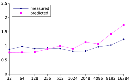
Figure 12: Precision of the statistical model.

In all cases, predicted performance is close to the actual performance. In $8$ out of $11$ data points, both lines are either above or below $1$, and the lock placement synthesized by O-Liss for these parameter values is indeed optimal.

These encouraging results experimentally justify our statistical performance model and the overall synthesis approach based on a combination of static program analysis and runtime profiling.

References

- [1] J. Alglave, D. Kroening, V. Nimal, and D. Poetzl. Don’t sit on the fence - A static analysis approach to automatic fence insertion. In CAV, pages 508–524, 2014.
- [2] Alberto Bertoni, Giancarlo Mauri, and Nicoletta Sabadini. Equivalence and membership problems for regular trace languages. In Automata, Languages and Programming, pages 61–71. Springer, 1982.
- [3] R. Bloem, G. Hofferek, B. Könighofer, R. Könighofer, S. Außerlechner, and R. Spörk. Synthesis of synchronization using uninterpreted functions. In FMCAD, pages 35–42, 2014.
- [4] P. Černý, K. Chatterjee, T. Henzinger, A. Radhakrishna, and R. Singh. Quantitative synthesis for concurrent programs. In CAV, pages 243–259, 2011.
- [5] P. Černý, E. Clarke, T. Henzinger, A. Radhakrishna, L. Ryzhyk, R. Samanta, and T. Tarrach. From non-preemptive to preemptive scheduling using synchronization synthesis. In CAV, page to appear, 2015.
- [6] P. Černý, T. Henzinger, A. Radhakrishna, L. Ryzhyk, and T. Tarrach. Efficient synthesis for concurrency by semantics-preserving transformations. In CAV, pages 951–967, 2013.
- [7] P. Černý, T. Henzinger, A. Radhakrishna, L. Ryzhyk, and T. Tarrach. Regression-free synthesis for concurrency. In CAV, pages 568–584. 2014. https://github.com/thorstent/ConRepair.
- [8] S. Cherem, T. Chilimbi, and S. Gulwani. Inferring locks for atomic sections. In Proceedings of the ACM SIGPLAN 2008 Conference on Programming Language Design and Implementation, Tucson, AZ, USA, June 7-13, 2008, pages 304–315, 2008.
- [9] J. Deshmukh, G. Ramalingam, V. Ranganath, and K. Vaswani. Logical Concurrency Control from Sequential Proofs. In Programming Languages and Systems, pages 226–245. 2010.
- [10] P. Diniz and M. Rinard. Lock coarsening: Eliminating lock overhead in automatically parallelized object-based programs. J. Parallel Distrib. Comput., 49(2):218–244, 1998.
- [11] M. Emmi, J. Fischer, R. Jhala, and R. Majumdar. Lock allocation. In POPL, pages 291–296, 2007.
- [12] A. Gupta, T. Henzinger, A. Radhakrishna, R. Samanta, and T. Tarrach. Succinct representation of concurrent trace sets. In POPL15, pages 433–444, 2015.
- [13] G. Jin, W. Zhang, D. Deng, B. Liblit, and S. Lu. Automated Concurrency-Bug Fixing. In OSDI, pages 221–236. 2012.
- [14] Memcached distributed memory object caching system. http://memcached.org.
- [15] A. Solar-Lezama, C. Jones, and R. Bodík. Sketching concurrent data structures. In PLDI, pages 136–148, 2008.
- [16] T. Usui, R. Behrends, J. Evans, and Y. Smaragdakis. Adaptive locks: Combining transactions and locks for efficient concurrency. J. Parallel Distrib. Comput., 70(10):1009–1023, 2010.
- [17] M. Vaziri, F. Tip, and J. Dolby. Associating synchronization constraints with data in an object-oriented language. In POPL, pages 334–345, 2006.
- [18] M. Vechev, E. Yahav, R. Raman, and V. Sarkar. Automatic verification of determinism for structured parallel programs. In SAS, pages 455–471, 2010.
- [19] M. Vechev, E. Yahav, and G. Yorsh. Abstraction-guided synthesis of synchronization. In POPL, pages 327–338, 2010.
- [20] Y. Zhang, V. Sreedhar, W. Zhu, V. Sarkar, and G. Gao. Minimum lock assignment: A method for exploiting concurrency among critical sections. In LCPC, pages 141–155, 2008.