Approximating W projection as a separable kernel
Abstract
W projection is a commonly-used approach to allow interferometric imaging to be accelerated by Fast Fourier Transforms (FFTs), but it can require a huge amount of storage for convolution kernels. The kernels are not separable, but we show that they can be closely approximated by separable kernels. The error scales with the fourth power of the field of view, and so is small enough to be ignored at mid to high frequencies. We also show that hybrid imaging algorithms combining W projection with either faceting, snapshotting, or W stacking allow the error to be made arbitrarily small, making the approximation suitable even for high-resolution wide-field instruments.
keywords:
techniques: interferometric – methods: numerical1 Introduction
In interferometric imaging, the relationship between sampled visibilities and the image plane is almost a Fourier transform, but with a term that depends on – the dot product of the baseline vector with the unit vector towards the phase centre. A number of approaches have been developed to deal with this troublesome term.
One of these is W projection (Cornwell et al., 2008), which converts the image-space multiplication by a phase screen into a convolution with its Fourier transform in space. This convolution is usually combined with an anti-aliasing filter, yielding a combined kernel, the Gridding Convolution Function (GCF), for which closed-form formulae are not known. Instead, the GCF is sampled in three dimensions and stored in a lookup table. Depending on the desired accuracy, these kernels can become excessively large. Apart from requiring large amounts of memory or disk space to store, this can also reduce performance as the samples are moved in and out of caches.
Our contribution is to recognize that the phase screen for a particular value of , and hence its Fourier transform, is very close to being separable, i.e., an outer product of two one-dimensional functions. By approximating the phase screen in this way, we can drastically reduce the storage required for lookup tables. Conversely, it allows for much finer sampling of the kernel in the same amount of memory, potentially improving accuracy.
Sec. 2 recaps the basics of W projection, and introduces the notation we use. In Sec. 3 we describe our separable approximation, and provide a theoretical analysis of the error. The error in position scales with the fourth power of the field of view, and so is acceptable for small to medium fields of view.
W projection can be combined with other imaging techniques, which we discuss in Sec. 4. We show that this allows the error to be reduced further, allowing our approach to be used even for wide fields of view. Sec. 5 discusses the effect on computation cost, and our conclusions are presented in Sec. 6.
2 Background and notation
We will focus mainly on transforming from sampled visibilities to a dirty image. Nevertheless, the same techniques and analysis apply to prediction of visibilities from a model image.
As usual, are baseline coordinates in a fixed coordinate system with in the direction of the phase centre. We measure in wavelengths rather than units of distance. The corresponding direction cosines are denoted , with . For compactness of notation, we will also use and interchangeably.
We will ignore direction-dependent effects, and assume a time- and baseline-independent perceived brightness distribution . Let the th visibility have coordinates , visibility value and weight . The dirty image is given by
| (1) |
The corresponding prediction of visibilities from a model is
| (2) |
Let and be its Fourier transform, and let . Then
| (3) | ||||
This is typically combined with an antialiasing kernel (with inverse Fourier transform ) to give
| (4) |
The two convolution kernels and are combined into a gridding convolution function (GCF) by multiplying their inverse Fourier transforms and , and taking the Fourier transform of the result.
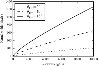
Generating a kernel is expensive, so usually they are either fully precomputed, or are generated on-demand then cached. The storage size is thus an important consideration. The antialiasing kernel is typically small (e.g., pixels), so the support of the GCF is dominated by the support of . The support (in -plane pixels) necessary to represent the function out to the fraction of the peak is (Mitchell & Bernardi, 2014)
| (5) |
Fig. 1 shows typical values of this function for .
Kernels can be hundreds of pixels across, even for baselines of a few kilometres. What is worse, they must be oversampled to avoid aliasing effects. A typical oversampling factor is 8 (Romein, 2012), which means that a single kernel may require millions of samples and thus consume tens of megabytes.
Cornwell et al. (2012) suggest that the number of planes should be
| (6) |
where is the tolerable loss of amplitude in the image plane due to decorrelation effects. This can easily reach at low elevations with , and storing all the kernels can require tens or even hundreds of gigabytes. Our method can reduce memory usage by a factor of 1000 or more, making precomputation practical.
3 Derivation and analysis
We aim to approximate as a separable function. We assume that the antialiasing function is separable, and hence it suffices to approximate as a separable function.
Recall that and . Using the Taylor expansion , we get
| (7) |
The first few terms of the phase depend on either or , but not both, and these are the dominant terms when . This is what makes approximately separable. Let
| (8) | ||||
| (9) |
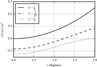
where is a tuning parameter we will discuss later. We approximate by . This approximation introduces an image-space phase error of
| (10) | ||||
Denote the factor inside the square brackets by . We would like to minimize over the image. The largest values will clearly be along the edges. Fig. 2 shows how varies along an edge for several values of . Ignoring the term, the value minimizes the maximum error at , while favors accuracy on the and axes and pushes the error into the corners.
We will now approximate the array as instantaneously co-planar (ignoring the slight curvature due to the shape of the Earth), so that can be computed as for some time-varying d. Note that ( being the elevation angle), so it is bounded by the minimum elevation. This allows us to recast the phase error as an instantaneous position error. When substituting the approximation into (3), we get
| (11) | ||||
If we can find such that
| (12) |
then the phase error is equivalent to shifting in the correct dirty image to l in the approximated dirty image. In other words, at a single point in time the approximation will cause a distortion in the image; as the Earth rotates, d will change, causing sources to be smeared out.
If is sufficiently small, then this error can reasonably be ignored. Cornwell et al. (2012) show that the relative loss in amplitude at l is proportional to , assuming a parabolic dirty beam, where is the resolution; it is thus desirable that . While (12) can be solved exactly (see Appendix A), we can obtain more insight from the approximation
| (13) |
which suggests that is sufficient.
We can translate this into a relationship between parameters of the instrument. The field of view is given by , where is the wavelength, is the antenna/station diameter, and is a constant that depends on the antenna (e.g., illumination tapering) and the desired field of view relative to the primary beam size. For example, gives an image that encloses the first null of an ideal Airy disk (Taylor et al., 1999, p. 41). For resolution we use the rule of thumb , where is the length of the longest baseline; the actual constant factor depends on the coverage and imaging weights (Taylor et al., 1999, p. 131). As noted above, . Thus,
| (14) |
To provide an example, let us consider some worst-case values for MeerKAT (Karoo Array Telescope) (SKA South Africa, 2015, 2014): (), , , gives , allowing for a large without problems.
Phase 1 of Square Kilometre Array mid-frequency instrument (SKA1-MID) will support lower frequencies and much longer baselines (SKA Organisation HQ, 2015): , , (). In this case, (14) gives , assuming the same minimum elevation as for MeerKAT. This means that the position error is of the same order as the beam size, which over time will cause decoherence at the edges of the image.
Due to the cubic dependence on , our basic approach is applicable at mid and high frequencies, but breaks down at lower frequencies. In general, we see limited value to the basic approach below about , at least for arrays of small dishes. However, combining W projection with other imaging approaches allows the error to be made arbitrarily small, making our approach suitable even at low frequencies. This is discussed further in Sec. 4.
It is interesting to note that the analysis above applies to other phase errors of the form . In particular, if no correction for W is done at all, then . Surprisingly, (13) does not depend on the array diameter or largest value, even though effects are conventionally associated with long baselines (Cornwell et al., 2008). Long baselines play an indirect role, in that they give high resolution and hence position errors are larger relative to the synthesized beam.
4 Combination with other techniques
W projection is only one approach to dealing with the term, and hence allowing Fast Fourier Transforms to be used to accelerate imaging. Others include faceting, snapshot imaging, and W stacking. In each case, it is possible to hybridize the algorithm with W projection to combine the computational strengths of both. W projection’s strength is in handling small values very accurately (limited only by sampling resolution), but it becomes computationally very costly to handle large values as the necessary support of the GCF grows. Hybrid techniques use alternative methods to make coarse phase corrections, with the finer corrections left to W projection.
Since the phase error in our method scales with , it seems likely that these hybrid methods would be particularly suitable since the values involved would be reduced. The following subsections show that this is indeed the case.
4.1 Faceting
Faceting has a number of advantages for imaging: each facet requires less working memory, and the reduction in field of view allows effects to be ignored or to be corrected more easily. Here we will discuss faceting in which the field of view of each facet is small, but not so small that effects can be completely ignored. This is an important domain, because there is a fixed cost per facet to adjust and grid the visibilities, and hence a large number of tiny facets can be computationally costly.
In classical faceting, the coordinate system is rotated and the phase of visibilities is adjusted so that each facet has its own phase centre. In terms of effects, each facet behaves as an independent image with a narrower field of view. Since the error scales with the fourth power of field of view, using even a small number of facets will greatly reduce the errors.
More recently, ‘image-plane’ faceting (Kogan & Greisen, 2009) applies a non-orthogonal change of coordinate system so that the facets are all part of a single plane tangent to the celestial sphere at the original phase centre, rather than each being tangent at the facet centre. This simplifies generation of a single image from the facets, but complicates our analysis.
Kogan & Greisen (2009) derive the equations for image-plane faceting using only a first-order Taylor approximation to the factor. In their derivation, all effects are corrected by suitable adjustments to u. For a hybrid W-projection/faceting algorithm, we must compute a second-order approximation.
Let , let be the facet centre, with , and let l refer to the position relative to the facet centre, such that the position relative to the original phase centre is . The modified correction is
| (15) |
We now approximate using a Taylor polynomial about :
| (16) | ||||
The initial term is absorbed into the coordinate transformation . The next two terms can be handled by a separable kernel, while the final term is not separable. We replace (9) by
| (17) | ||||
| (18) | ||||
| (19) |
There are a few noteworthy differences from the case of classical faceting. First, the component functions are now facet-dependent, and different for and . We have also used a lower-order approximation, because without being able to incorporate the term, there is little point in trying to compute higher-order terms. This also means that for a given total field of view, the error now only scales with the square rather than the fourth power of the facet width.
Fig. 3 shows the position error at elevation and a field of view, using and grids of facets. In the case, the error is reduced by an order of magnitude compared to the unfaceted approach. However, the discontinuities at the boundaries between facets may be problematic, since a source on a boundary will appear in different positions in the two facets.
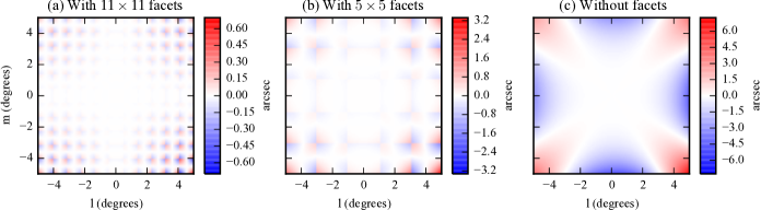
Our claim that the error scales quadratically with facet size holds between 3a and 3b, but 3c does not follow the same scaling. This is for two reasons. Firstly, 3c uses (9) rather than (19), and the former partially corrects for fourth-order errors. Secondly, the claim only holds for facets with the same centre; since 3c has the facet centre at the phase centre, the errors are smaller.
4.2 W snapshots
Snapshot imaging corrects the position error introduced by terms in image space. Since the position error is time-varying, an image is created for a small window of time, then reprojected to correct the distortions. Over a longer observation, many images are made and added together. For each snapshot, a single value is found such that , and then after creating the image, the image is reprojected so that is mapped to l.
W snapshots (Cornwell et al., 2012) is a hybrid method combining snapshot imaging with W projection. The snapshot warping corrects for an average position error over the snapshot duration, while W projection fixes up residual errors caused by long snapshots or by non-planar arrays. This allows the snapshot duration to be much longer than for traditional snapshot imaging, while still reducing the gridding costs by keeping values small.
The component of the phase is absorbed into the reprojection, leaving a residual of to be handled by W projection111For analysis we will assume a coplanar array, but deviations from planarity will also appear in the residual.. It follows that the remaining position error from using a separable kernel is
| (20) |
There is another source of phase error, not discussed by Cornwell et al. (2012): W projection does not account for the reprojection222This could be fixed by generating a custom kernel for each value of . We have not analyzed this approach., and hence the actual phase correction applied is . This will introduce a phase error of
| (21) | ||||
For comparison, the phase error associated with separation of the kernel, when and , is approximately . Unless the phase centre is close to the zenith, , and so the error due to separation will be insignificant compared to this other error. Of course, both errors can be made arbitrarily small by limiting the snapshot length, although in the limit the assumption of a coplanar array will break down.
4.3 W stacking
W stacking (Offringa et al., 2014) is similar to snapshot imaging in that visibilities are partitioned, and within each partition the average effects are corrected in image space. Instead of partitioning visibilities by time, they are partitioned by , and the image-space adjustment is a phase correction rather than a reprojection. As with snapshotting, it is possible to use coarser partitioning, and hence fewer Fourier transforms, by using W projection to deal with residual terms.
Unlike in the previous cases, the projection term is no longer directly correlated with u at a point in time. The errors will thus cause smearing rather than a systematic shift in position. Let be the residual that will be adjusted by projection. If the slices are evenly spaced apart, then . With sufficiently many slices, can be treated as a uniformly-distributed random variable.
A phase error of will cause a relative amplitude loss of at the position of a point source. Hence, the expected loss of amplitude is
| (22) | ||||
Let us re-evaluate the SKA1-MID example from Sec. 3, with a field of view (corresponding very roughly to the second null of the primary beam). In this case, everywhere in the image, so provided that , the loss in amplitude will be minimal. At , the longest baseline is wavelengths, so this will not require an unreasonable number of slices.
A potential issue with a core-heavy array is that if the slice is too wide, it will contain a substantial fraction of the visibilities. These visibilities contribute to the dirty image exactly as if no W stacking was applied, and hence create a ghost source at as in equation (12). This suggests placing a large number of slices close to , with wider-spaced slices at larger values. Adapting slice width to the visibility density will also reduce computation time, because narrow slices need less support for the convolution kernel, hence speeding up gridding, but sparse regions benefit from fewer, wider slices to reduce Fourier transform costs.
5 Computation cost
With our approach, the gridding convolution function becomes a separable function . Updating the grid cell at with visibility now requires computing rather than . This would appear to require double the number of multiplications. However, the partial product depends only on and not , and hence can be computed once and reused for every value of in the support of the kernel. The number of multiplications thus only increases by a factor of , where is the width of the kernel in grid cells.
It is also important to emphasize that floating-point operations are not necessarily the bottleneck in gridding: Romein (2012) and Muscat (2014) both report that performance is limited by the memory system in their respective GPU-accelerated gridders. Muscat reports that loading the kernel data from texture memory is the limiting factor, and our smaller kernel is likely to improve cache efficiency here. Our prototype GPU gridder using a separable kernel achieves greater efficiency than the published figures for either of these implementations, but further work is required to establish whether this is due to other factors.
6 Conclusions and future work
We have demonstrated a method to approximate the GCF for W projection which reduces the lookup table from three to two dimensions, leading to a massive reduction in memory. This makes it possible to store more planes, to make better usage of caches, and possibly to keep the entire kernel in a smaller but faster level of a memory hierarchy. We have focused on dirty imaging, but the same approximation can be used for prediction, allowing for Cotton–Schwab major cycles (Schwab, 1984).
The approximation introduces a phase error, which is linear in and hence translates to an instantaneous position error for a coplanar array. The error is small, scaling with the fourth power of the field of view. The approach is thus practical for mid- and high-frequency dish arrays, even with pure W projection, provided that baselines are no more than a few tens of kilometres long. The error can also be made arbitrarily small by using faceting, snapshotting or W stacking with a sufficient number of facets, snapshots or stack slices. This allows the basic idea to be extended to higher resolutions and lower frequencies, such as is envisioned for SKA1-MID. It remains future work to investigate whether wide-field, low-frequency aperture arrays can be supported without requiring an excessively large number of facets/snapshots/slices that would harm the overall performance.
While we believe that our approach will increase performance due to reduced pressure on memory systems, we have not yet implemented both versions of the kernel in a single gridding application to provide a fair comparison.
An idea that merits further investigation is to obtain better accuracy by storing and applying the correction . This will potentially require far less support and/or sampling rate than the original GCF, and hence can be stored in a small yet full-dimension table. It may also be possible to approximate this correction as another separable function, but rotated to the original.
Another method used in interferometric imaging is A projection, in which primary beam correction is done in the plane by convolution (Bhatnagar et al., 2006). This may also be combined with W projection, and one may naturally ask whether our technique can be applied to the combination. Unfortunately this is unlikely to be as successful, as the primary beam rotates on the sky and is unlikely to be separable in all orientations. Our technique can still be used with other approaches to primary beam correction, such as image-space correction for each snapshot with W snapshots.
References
- Bhatnagar et al. (2006) Bhatnagar S., Golap K., Cornwell T., 2006, Correction of Errors due to Antenna Power Patterns during Imaging, EVLA memo 100
- Cornwell et al. (2008) Cornwell T., Golap K., Bhatnagar S., 2008, IEEE J. of Selected Topics in Signal Processing, 2, 647
- Cornwell et al. (2012) Cornwell T. J., Voronkov M. A., Humphreys B., 2012, Proc. SPIE, 8500, 85000L
- Kogan & Greisen (2009) Kogan L., Greisen E. W., 2009, Faceted imaging in AIPS, AIPS memo 113
- Mitchell & Bernardi (2014) Mitchell D., Bernardi G., 2014, Analysis of w-projection kernel size, SKA SDP Consortium document SKA-TEL-SDP-IMG-Wkernels
- Muscat (2014) Muscat D., 2014, Master’s thesis, University of Malta
- Offringa et al. (2014) Offringa A. R., et al., 2014, MNRAS, 444, 606
- Romein (2012) Romein J. W., 2012, in Proc. 26th ACM Int. Conf. on Supercomputing. ICS ’12. ACM, New York, NY, USA, pp 321–330
- SKA Organisation HQ (2015) SKA Organisation HQ 2015, The world’s largest radio telescope takes a major step towards construction, https://www.skatelescope.org/news/worlds-largest-radio-telescope-near-construction/
- SKA South Africa (2014) SKA South Africa 2014, South Africa’s MeerKAT Radio Telescope, https://docs.google.com/a/ska.ac.za/viewer?a=v&pid=sites&srcid=c2thLmFjLnphfHB1YmxpY3xneDo3Yjg5ODU3ZGYxMjI4NDg0
- SKA South Africa (2015) SKA South Africa 2015, MeerKAT Array Releases and Specifications, http://public.ska.ac.za/meerkat/schedule
- Schwab (1984) Schwab F. R., 1984, Astron. J., 89, 1076
- Taylor et al. (1999) Taylor G. B., Carilli C. L., Perley R. A., eds, 1999, Synthesis Imaging in Radio Astronomy II Astronomical Society of the Pacific Conference Series Vol. 180
Appendix A Proof of approximation for
Here we will derive an exact solution to (12) and justify the approximation given in (13). Rearranging (12) gives
| (23) |
It is immediately clear that is a multiple of d, so let . Let
| (24) |
Then
| (25) | |||||
| (26) | |||||
| (27) | |||||
| (28) | |||||
| (29) |
This is a quadratic equation in , which can easily be solved. It is possible that both two roots satisfy (26), but we are only interested in the one with the smaller absolute value.
We now turn to approximating . To get an initial estimate, we ignore the term , giving To improve this, we note that
| (30) | ||||
where the approximation is a linear Taylor polynomial around . Substituting this back into (23) gives
| (31) |
and if we use in place of in the right-hand side, we get the improved approximation
| (32) |