Pseudo-Gauss distribution:
a reversible counterpart of the true turbulent velocity gradient distribution
A.V. Kopyev,^1,   K.P. Zybin^1,2,
1 P.N. Lebedev Institute of Physics, Theory Department, 119991 Moscow, Russia
² Higher School of Economics, Mathematical Department, 101000 Moscow, Russia

Abstract

On the grounds of both widely known experimental and numerical data of the strain-rate tensor statistical properties in the fully developed incompressible turbulent flow and the integral transformations deduced in the article, some important statistical properties of the flow, known as kinematical, are found to be dynamical (i.e. taking place purely in a turbulent flow). A new pseudo-Gauss distribution is introduced in the article and, as a consequence of these properties, a considerable feature distinguishing this distribution from the Gauss one is found to be the general feature of the turbulent statistics. Thus, the new distribution is proved to be a reversible counterpart of the true turbulent velocity gradient distribution instead of the Gauss one.

1.Introduction

The velocity field in the fully developed turbulent flow is known to be stochastic. Its statistical properties have attracted the interest of researchers in physics, mechanics and mathematics for more than a century, but the problem is still far from being solved. Previously, a new model [1], which gives a physical interpretation of the known multifractal model, was formulated. The large-scale velocity gradients play a significant role in this model. Now, we try to focus our interest on the statistical properties of the velocity gradients in the fully-developed turbulent flow.

Full velocity gradient statistical description

Velocity gradients compose the tensor, which can be defined as value $A_{ij}$ in a given point $\vec{x}_{0}$ from the following expansion of the velocity field in $\vec{x}_{0}$ neighborhood:

$$u_{i}\left(\vec{x}\right)=u_{i}\left(\vec{x}_{0}\right)+A_{ij}\left(\vec{x}_{0}\right)\left(x_{j}-{x_{0}}_{j}\right)+O\left(|\vec{x}-\vec{x}_{0}|^{2}\right)$$ (1)

This tensor is called the velocity gradient tensor and as it is evident from (1):

$$A_{ij}\left(\vec{x}_{0}\right)=\dfrac{\partial u_{i}}{\partial x_{j}}|_{\vec{x}=\vec{x}_{0}}$$ (2)

It follows from the incompressibility of the flow that the trace of the velocity gradient tensor is equal to zero:

$$A_{ii}=0$$ (3)

Under these conditions, the velocity gradient tensor has 8 independent components. It has 5 rotational invariants which are independent of the frame orientation. For instance, the invariants can be chosen as [2]:

$$Q=-\dfrac{1}{2}A_{im}A_{mi}\;\;\;\;R=-\dfrac{1}{3}A_{im}A_{mn}A_{ni}$$ (4)

$$Q_{S}=-\frac{1}{2}S_{im}S_{mi}\;\;\;\;R_{S}=-\frac{1}{3}S_{im}S_{mn}S_{ni}$$ (5)

$$V^{2}=S_{in}S_{im}\omega_{m}\omega_{n}$$ (6)

Here $S_{ij}$ is a strain-rate tensor and $\vec{\omega}$ - vorticity of the flow. They are both components of the velocity tensor and can be defined by decomposition:

$$A_{ij}=\frac{1}{2}\left(A_{ij}+A_{ji}\right)+\frac{1}{2}\left(A_{ij}-A_{ji}\right)=S_{ij}-\frac{1}{2}\epsilon_{ijm}\omega_{m}$$ (7)

Here $\epsilon_{ijm}$ is the antisymmetric tensor. Because of $SO(3)$ symmetry the probability density functions (PDFs) of velocity gradients depend on rotational invariants only [3]. It could be expressed in terms of invariants (4)-(6) or in any other five independent invariants, which are functions of invariants (4)-(6).

Symmetric velocity gradients statistical description

This article focuses on the statistical properties of the symmetrical part of decomposition (7). One can see from (5) that invariants $Q_{S}$ and $R_{S}$ are functions of strain-rate tensor $S_{ij}$ only. Due to the incompressibility and symmetrical arguments $S_{ij}$ has only two invariants which are independent of the frame orientation. Thus, the statistical properties of strain-rate tensor $S_{ij}$ can be considered independently in terms of $Q_{S}$ and $R_{S}$ invariants or in other two independent invariants, which must be functions of $Q_{S}$ and $R_{S}$. For instance, new invariants, namely, the maximum $\left(\lambda_{1}\right)$ and the minimum $\left(\lambda_{3}\right)$ eigenvalues of strain-rate tensor $S_{ij}$ could be chosen instead of $Q_{S}$ and $R_{S}$ (due to the incompressibility, the third eigen value $\lambda_{2}$, which is greater than $\lambda_{3}$ but less than $\lambda_{1}$, is equal to $-\lambda_{1}-\lambda_{3}$). The expressions of $Q_{S}$ and $R_{S}$ in terms of $\lambda_{1}$ and $\lambda_{3}$ take the form:

$$Q_{S}=-\left(\lambda_{1}^{2}+\lambda_{1}\lambda_{3}+\lambda_{3}^{2}\right)$$ (8)

$$R_{S}=\lambda_{1}\lambda_{3}\left(\lambda_{1}+\lambda_{3}\right)$$ (9)

The inverse transform to (8), (9) can be shown to be unique, but much more complicated.

There are other parameters, single PDFs of which do not give the full statistic information of the strain but are useful in considering of fluid particle deformation tendencies.

$$\beta=\dfrac{\sqrt{6}\lambda_{2}}{\sqrt{\lambda_{1}^{2}+\lambda_{2}^{2}+\lambda_{3}^{2}}}$$ (10)

$$s=\dfrac{-3\sqrt{6}\lambda_{1}\lambda_{2}\lambda_{3}}{\left(\lambda_{1}^{2}+\lambda_{2}^{2}+\lambda_{3}^{2}\right)^{\frac{3}{2}}}$$ (11)

They were introduced and analyzed in articles [4, 5] respectively. In an incompressible flow both of them can change in the interval $\left[-1;1\right]$. Each of these values gives a unique value of eigenvalues ratio $\lambda_{1}:\lambda_{2}:\lambda_{3}$ but says nothing about their absolute values. The expression coupling two parameters $\beta$ and $s$ has been given in the article [5], so they cannot be chosen as two independent parameters of $S_{ij}$ and, thus, it is surely senseless to find the joint PDF of the parameters.

Physical interpretation of velocity gradients

Note that defined tensors $A_{ij}$ and $S_{ij}$, vorticity vector $\vec{\omega}$ and the $S_{ij}$ eigen values (with the corresponding eigen vectors) have a physical interpretation in terms of fluid particles - macroscopic but small volumes of the moving flow. Let $\vec{x}_{0}$ in (2) be the position vector of the fluid particle center of mass. If the fluid particle dimensions are small enough to apply the linear expansion (1), velocity gradient tensor $A_{ij}$ entirely governs its dynamics in its center-of-mass system in a given moment: the rotation and the deformation of the particle are governed by vorticity vector $\vec{\omega}$ and strain-rate tensor $S_{ij}$ accordingly. As for the deformation of the fluid particle, three principal axes of the strain can be distinguished in the directions of $S_{ij}$ eigen vectors with the exponential rate of strain in these directions. Namely, the expansion with relative rate $\lambda_{1}$ occurs in the direction of the eigen vector corresponding to these directions, the contraction with rate $|\lambda_{3}|$ in its eigen vector direction and either the expansion or the contraction (depending on the sign of $\lambda_{2}$) with rate $|\lambda_{2}|$ take place in the corresponding eigen vector direction [6]. Hence, the ratio $\lambda_{1}:\lambda_{2}:\lambda_{3}$ (either parameter $\beta$ or $s$) characterizes the shape of the ellipsoidal deformation of an initially spherical fluid particle. For example, if $\beta=+1$ (or $s=+1$) then $\lambda_{1}:\lambda_{2}:\lambda_{3}=1:1:-2$ and the initially spherical fluid particle becomes a pancake-like. If $\beta=-1$ (or $s=-1$) then $\lambda_{1}:\lambda_{2}:\lambda_{3}=2:-1:-1$ and it tends to be a filament.

Generalization of velocity gradients on large scales

If we consider so large fluid particles that the expansion (1) becomes wrong, the velocity gradient tensor, defined in (2), fails to govern their dynamics. However, it is those particles, which are known to be of huge interest in the turbulence theory [7]. Therefore, the definition of the velocity gradient tensor (in [8] it is called ”true” velocity gradient tensor) should be generalized on different scales, for example, with the help of the following averaging:

$$A_{ij}^{R}\left(\vec{x}_{0}\right)=\dfrac{1}{V^{R}}\int_{V^{R}}A_{ij}\left(\vec{x}_{0}+\vec{r}\right)d\vec{r}$$ (12)

Where $V^{R}$ is the spherical volume with the center in the point $\vec{x}_{0}$ , which radius is equal to $R$. It is possible to split generalizing tensor $A_{ij}^{R}$ into symmetrical and antisymmetric parts $S_{ij}^{R}$ and $-\frac{1}{2}\epsilon_{ijm}\omega_{m}^{R}$ analogous to $A_{ij}$ (7). The traces of tensors $A_{ij}^{R}$ and $S_{ij}^{R}$ are obviously equal to zero, so it has five and two nonzero orientation invariants respectively, which are defined in the same way as it was done previously. Therefore, general statistical analysis is analogous for both true and generalized gradient tensors. Due to this, the results deduced in the article are valid for both tensors.

Short overview of the previous results

All above discussed quantities were calculated in many direct numerical simulations (DNS) and were measured in a wide range of experiments (see the overview [9] and the references in it). There are also many phenomenological theoretical models for these quantities (see the overview [2] and the references in it). Note that most of numerical, experimental and theoretical articles on the velocity gradients deal with joint PDF of $Q$ and $R$ velocity gradient tensor invariants ([2, 9] and references).

Concerning strain-rate tensor invariants, note that DNS are usually focused on the joint PDF of invariants $Q_{S}$ and $R_{S}$ (e.g. [10, 11]) and, on the contrary, in experiments researchers usually prefer to measure single distributions of $\lambda_{1}$, $\lambda_{2}$ and $\lambda_{3}$ (e.g. [12, 13]). Single $\beta$ and $s$ PDFs were measured and calculated in a considerable amount of various fully developed incompressible and slightly compressible flows. Their properties has been investigated since they were calculated with low Reynolds numbers ($\beta$ [4, 5, 14, 15], $s$ [5]) and measured by hot-wire probes ($\beta$ [16]). There are modern precise calculations ($\beta$ [8, 17], $s$ [17]) and measurements by both hot-wire probes ($\beta$ and $s$ [17]) and PIV methods ($\beta$ [8]). The important property of $\beta$ PDF is that it vanishes at the end points of its domain (i.e. at points $\beta=\pm 1$). It can be shown [5] that this means $s$ PDF boundedness at $s=\pm 1$, which are end points of its domain.

Present article results

In contradiction to the known results of the article [5], we will show that the properties of single $\beta$ and $s$ PDFs give non-trivial information about turbulent statistics (see section 4). Before this, in section 3, we will show that in case of the Gauss velocity distribution these properties do not take place (i.e. $\beta$ PDF does not vanish at $\beta=\pm 1$ and $s$ PDF tends to infinity in $s=\pm 1$) and will give the reversibility analog of the Gauss distribution that we have called the pseudo-Gauss distribution, for which these properties take place. All the results will be found by means of the integral transformations between different PDFs that we will deduce in section 2. Note that it is convenient to give the resulting property of turbulent statistics not only in terms of invariants $Q_{S}$ and $R_{S}$ but also via ”shuffled” eigenvalues of the strain-rate tensor and their joint PDF, which we will introduce in section 2.

In our opinion, the contradiction of our results with the previous ones is associated with our account of pre-exponential factor in the joint PDF of invariants $Q_{S}$ and $R_{S}$ in Gauss case, which has not been accounted before (see section 3).

2.Joint and single PDFs of different strain-rate tensor invariants and relations between them

”Shuffled” and ”ordered” eigen values

Let $\lambda_{1}$, $\lambda_{2}$ and $\lambda_{3}$ be eigen values of the strain-rate tensor $S_{ij}$ ordered by the condition $\lambda_{1}\geq\lambda_{2}\geq\lambda_{3}$ as they are defined in the introduction. Let us introduce the procedure, which we call ”shuffling”. This means that we set the ”ordered” eigenvalues $\lambda_{1}$, $\lambda_{2}$ and $\lambda_{3}$ into one-to-one correspondence with so-called ”shuffled” eigenvalues $\mu_{1}$, $\mu_{2}$ and $\mu_{3}$ letting each be equal to one of three $\lambda_{i}$ with the same probability $\frac{1}{3}$. Due to the one-to-one correspondence, it is evident that the shuffled eigenvalues hold the incompressibility condition $\mu_{1}+\mu_{2}+\mu_{3}=0$, too. Moreover, two of the shuffled eigen values (e.g. $\mu_{1}$ and $\mu_{2}$) can be marked as new strain-rate tensor invariants like $Q_{S}$ and $R_{S}$ or $\lambda_{1}$ and $\lambda_{3}$. Thus, as we have mentioned in introduction, PDFs of the functions depending on the strain-rate tensor can be expressed in terms of shuffled eigen values.

Joint PDFs of the shuffled eigen values ($\mu$ PDFs)

Let us denote the joint PDF of the shuffled eigen values $\mu_{i}$ and $\mu_{j}$ ($i\neq j$) $f_{ij}\left(x,y\right)$. By the construction of the procedure we have 4 simple properties for $\mu$ PDFs:

• $\mathrm{Domain}\left[f_{ij}\left(x,y\right)\right]=\mathbb{R}^{2}$

• $f_{ij}\left(x,y\right)=f_{ji}\left(x,y\right)$

• $f_{12}\left(x,y\right)=f_{23}\left(x,y\right)=f_{13}\left(x,y\right)$

• $f_{ij}\left(x,y\right)=f_{ij}\left(y,x\right)=f_{ij}\left(x,-x-y\right)$

These properties make ”shuffled” eigenvalues more convenient than the ordered ones and we will use them and their joint PDF hereafter. The inverse relations between the shuffled eigen values and the ordered ones are explicit and are given by the formulas:

$$\lambda_{1}=\max\left(\mu_{1},\mu_{2},-\mu_{1}-\mu_{2}\right)$$ (13)

$$\lambda_{3}=\min\left(\mu_{1},\mu_{2},-\mu_{1}-\mu_{2}\right)$$ (14)

Thus, the given procedure is reversible. The four properties of the $\mu$ PDFs can be taken into account by only considering the following functions:

$$f_{ij}\left(x,y\right)=\phi\left(-\left(x^{2}+xy+y^{2}\right),xy(x+y)\right)$$ (15)

where $\left(x;y\right)\in\mathbb{R}^{2}$.

Joint $Q_{S}$ and $R_{S}$ PDF

Let us find the relation between introduced PDF $f_{ij}\left(x;y\right)$ and joint $Q_{S}$ and $R_{S}$ PDF $f_{Q_{S}R_{S}}$ . Invariants $Q_{S}$ and $R_{S}$ are expressed by $\mu_{i}$ and $\mu_{j}$ for any $i$ and $j$ ($i\neq j$) in the following way:

$$\left\{\begin{aligned} Q_{S}&=-\left(\mu_{i}^{2}+\mu_{i}\mu_{j}+\mu_{j}^{2}\right)\\ R_{S}&=\mu_{i}\mu_{j}\left(\mu_{i}+\mu_{j}\right)\end{aligned}\right.$$ (16)

One can show that exactly six pairs of $\mu_{i}$ and $\mu_{j}$ correspond to one pair of values $Q_{S}$ and $R_{S}$. This divides the space $\left(\mu_{i};\mu_{j}\right)$ in 6 independent sectors, separated from each other by the lines on which two of the three eigenvalues are equal:

$$\left\{\begin{aligned} &\mu_{i}=\mu_{j}\\ &\mu_{i}=-\mu_{i}-\mu_{j}\\ &\mu_{j}=-\mu_{i}-\mu_{j}\end{aligned}\right.$$ (17)

The domain of $Q_{S}$ and $R_{S}$ ($D_{Q_{S}R_{S}}$), which is shown in Fig.1, is bounded by the curves $R_{S}=\pm\frac{2}{3\sqrt{3}}\left(-Q_{S}\right)^{\frac{3}{2}}$ in the lower half plane [10, 11]. To find the relation between the introduced joint PDF and the joint PDF of $Q_{S}$ and $R_{S}$ invariants the Jacobian of the transformation (16) is needed. Then:

$$f_{Q_{S}R_{S}}\left(q;r\right)=6\cdot\phi\left(q;r\right)\begin{Vmatrix}\dfrac{\partial\left(\mu_{i},\mu_{j}\right)}{\partial\left(Q_{S},R_{S}\right)}\end{Vmatrix}_{Q_{S}=q;R_{S}=r}=\dfrac{6\cdot\phi\left(q;r\right)}{\sqrt{-4q^{3}-27r^{2}}}$$ (18)

Where 6 is the number of $\mu_{i}$ and $\mu_{j}$ pairs, which correspond to the pair of values $Q_{S}$ and $R_{S}$ from (16). Also note that $\left(Q_{S};R_{S}\right)\in D_{Q_{S}R_{S}}$.

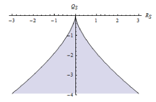
Figure 1: $D_{Q_{S}R_{S}}$: the domain of $Q_{S}$ and $R_{S}$ invariants

Hence, knowing $\mu$ PDF we can find the $Q_{S}$ and $R_{S}$ PDF by applying (18). From (16) and (18) we get the inverse relation:

$$f_{ij}\left(x;y\right)=\\ =\dfrac{|\left(x-y\right)\left(2x+y\right)\left(x+2y\right)|}{6}f_{Q_{S}R_{S}}\left(-\left(x^{2}+xy+y^{2}\right),xy(x+y)\right)$$ (19)

where $\left(x;y\right)\in\mathbb{R}^{2}$.

Single $s$ PDF

Using (11), it is possible to get $s$ PDF $f_{s}$ from $f_{Q_{S}R_{S}}$. It can be done by the integral transformation:

$$f_{s}\left(y\right)=\int_{-\infty}^{0}dq\int_{-\frac{2}{3\sqrt{3}}\left(-q\right)^{\frac{3}{2}}}^{\frac{2}{3\sqrt{3}}\left(-q\right)^{\frac{3}{2}}}f_{Q_{S}R_{S}}\left(q;r\right)\delta\left(y-\dfrac{3\sqrt{3}r}{2\left(-q\right)^{\frac{3}{2}}}\right)dr$$ (20)

Here $\delta\left(y-g\left(q;r\right)\right)$ is Dirac delta function on the surface $g\left(q;r\right)$ [24] convoluting with $f_{Q_{S}R_{S}}$ in its domain $D_{Q_{S}R_{S}}$, which is shown in Fig. 1. The calculation (20) could be reduced to the following expression:

$$f_{s}\left(y\right)=\frac{4}{3\sqrt{3}}\int_{0}^{+\infty}f_{Q_{S}R_{S}}\left(-t^{2};t^{3}\frac{2y}{3\sqrt{3}}\right)t^{4}dt$$ (21)

where $s\in\left[-1;1\right]$. From the transformation (21) and (18) the similar transformation between the $s$ PDF and the $\mu$ PDF could be determined:

$$f_{s}\left(y\right)=\frac{4}{\sqrt{3}\sqrt{1-y^{2}}}\int_{0}^{+\infty}\phi\left(-t^{2};t^{3}\frac{2y}{3\sqrt{3}}\right)tdt$$ (22)

Single $\beta$ PDF

Now, let us find analogous integral transformations for parameter $\beta$. To do it, let us use the explicit relations between parameters $\beta$ and $s$ given in [5]:

$$\left\{\begin{aligned} &\beta=2\sin{\left(\frac{1}{3}\arcsin{s}\right)}\\ &s=\beta\left(3-\beta^{2}\right)/2\end{aligned}\right.$$ (23)

Determining the Jacobian of transformation (23) and using (21) we can find:

$$f_{\beta}\left(z\right)=f_{s}\left(\frac{z\left(3-z^{2}\right)}{2}\right)\begin{vmatrix}\dfrac{ds}{d\beta}\end{vmatrix}_{\beta=z}=\\ =\frac{2}{\sqrt{3}}\left(1-z^{2}\right)\int_{0}^{+\infty}f_{Q_{S}R_{S}}\left(-t^{2};t^{3}\frac{z\left(3-z^{2}\right)}{3\sqrt{3}}\right)t^{4}dt$$ (24)

where $z\in\left[-1;1\right]$. Analogously we can determine the integral transformation from joint PDF $\phi$ to PDF $f_{\beta}$:

$$f_{\beta}\left(z\right)=\frac{4\sqrt{3}}{\sqrt{4-z^{2}}}\int_{0}^{+\infty}\phi\left(-t^{2};t^{3}\frac{z\left(3-z^{2}\right)}{3\sqrt{3}}\right)tdt$$ (25)

3. Gauss and pseudo-Gauss distribution

Gauss distribution case

Let us consider the random velocity field with Gauss statistics. In the article ([25] Appendix B) it was shown that from the Gaussian distribution of the flow velocity follows the Gaussian distribution of the velocity gradient tensor elements. From the form given in [25] one can write for the strain-rate tensor eigen values PDF:

$$f_{ij}\left(x;y\right)=\phi\left(-\left(x^{2}+xy+y^{2}\right)\right)=\frac{\sqrt{3}}{2\pi M^{2}}\exp{\left(\dfrac{-x^{2}-xy-y^{2}}{M^{2}}\right)}$$ (26)

Here $M$ is a parameter characterizing the distribution dispersion, which in the incompressible case is governed only by the mean value of squared vorticity $\omega^{2}$ [25]. To find $Q_{S}$ and $R_{S}$ joint PDF let us take into account (18):

$$f_{Q_{S}R_{S}}\left(q;r\right)=\dfrac{3\sqrt{3}\exp{\left(q/M^{2}\right)}}{\pi M^{2}\sqrt{-4q^{3}-27r^{2}}}$$ (27)

Substitution (26) in (25) and (22) gives $\beta$ and $s$ PDFs for the Gauss velocity distribution:

$$f_{\beta}\left(z\right)=\dfrac{3}{\pi\sqrt{4-z^{2}}}$$ (28)

$$f_{s}\left(y\right)=\dfrac{1}{\pi\sqrt{1-y^{2}}}$$ (29)

These PDFs are shown in Fig. 2. We see that in this case $f_{\beta}$ does not vanish at the points $\pm 1$ as it was concluded in [5] (see figure 1 from [5]). Moreover, in contrast with [5] $f_{s}$ becomes infinity in the points $\pm 1$. In our opinion, this contradiction is associated with our account of pre-exponential factor $\left(-4q^{3}-27r^{2}\right)^{-1/2}$ in (27), which was not accounted before. To prove this statement we now consider $Q_{S}$ and $R_{S}$ joint PDF without the pre-exponential factor.

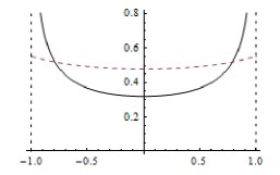
Figure 2: PDFs $f_{s}$ (the full curve with the vertical asymptotes) and $f_{\beta}$ (the dotted curve) in case of Gauss velocity field.

Pseudo-Gauss distribution case

Now let us consider the case of symmetric exponential distribution $f_{Q_{S}R_{S}}$ (without the pre-exponential factor) that we have called a pseudo-Gauss distribution:

$$f_{Q_{S}R_{S}}\left(q;r\right)=\dfrac{\sqrt{3}\exp{\left(q/A^{2}\right)}}{\sqrt{\pi}A^{5}}$$ (30)

In contrast to $M$ from (26), parameter $A$ still has no intuitive physically meaningful interpretation because we do not have the pseudo-Gauss distribution as a consequence of any specific velocity field like in the previous subsection. The inverse problem of finding the velocity distribution from distribution (30) is not considered in the present article and the question still remains open.

By substituting (30) in (19) we have:

$$f_{ij}\left(x;y\right)=\dfrac{\sqrt{3}\left|\left(x-y\right)\left(2x+y\right)\left(2y+x\right)\right|}{6\sqrt{\pi}A^{5}}\exp{\left(\dfrac{-x^{2}-xy-y^{2}}{A^{5}}\right)}$$ (31)

One can see that this $f_{ij}$ has a very specific shape as it vanishes on the lines $x=y$, $x=-x-y$ and $y=-x-y$, that is, when two of three strain-rate eigenvalues are equal $\beta=\pm 1$ (or $s=\pm 1$). Using (21), (24) and (30) after some developments, we have:

$$f_{\beta}\left(z\right)=\frac{3}{4}\left(1-z^{2}\right)$$ (32)

$$f_{s}\left(y\right)=\frac{1}{2}$$ (33)

Derived PDFs $f_{\beta}$ and $f_{s}$ (Fig. 3) are exactly the same as the ones in figure 1 in the article [5].

Figure 3: PDFs $f_{s}$ (the full curve) and $f_{\beta}$ (the dotted one) in case of pseudo-Gauss velocity field.

$Q$-distribution cases

Let us notice that there is no parameter $M$ in expressions (28) and (29), so, $f_{\beta}$ and $f_{s}$ are independent of the dispersion in (26). We now show that, moreover, the distributions (28) and (29) are valid not only for the Gauss distribution case, but for all symmetric PDFs $f_{ij}$.

Statement 1. If $\phi\left(q;r\right)=\phi\left(q\right)$, then $f_{s}\left(y\right)=1/{\pi\sqrt{1-y^{2}}}$ and $f_{\beta}\left(z\right)=3/{\pi\sqrt{4-z^{2}}}$

Indeed, it follows from (22):

$$f_{s}\left(y\right)=\frac{4}{\sqrt{3\left(1-y^{2}\right)}}\int_{0}^{+\infty}\phi\left(-t^{2}\right)tdt$$ (34)

Since the integral from the right side does not depend on $y$ and PDF $f_{s}\left(y\right)$ is normalized, the integral must fail to be governed by function $\phi\left(q\right)$:

$$\int_{0}^{+\infty}\phi\left(-t^{2}\right)tdt=\frac{\sqrt{3}}{4}\left(\int_{-1}^{1}\dfrac{dy}{\sqrt{1-y^{2}}}\right)^{-1}=\frac{\sqrt{3}}{4\pi}$$ (35)

This leads to the equation for $f_{s}\left(y\right)$. In the same manner, from (25) we easily can prove the one for $f_{\beta}\left(z\right)$:

$$f_{\beta}\left(z\right)=\frac{4\sqrt{3}}{\sqrt{4-z^{2}}}\int_{0}^{+\infty}\phi\left(-t^{2}\right)tdt=\frac{3}{\pi\sqrt{4-z^{2}}}$$ (36)

The analogous notation can be made about parameter $A$ in (30) and distributions (32) and (33), which are independent of it. Let us prove that distributions (32) and (33) take place not only in the pseudo-Gauss case but also for all symmetric PDFs $f_{Q_{S}R_{S}}$:

Statement 2. If $f_{Q_{S}R_{S}}\left(q;r\right)=f_{Q_{S}R_{S}}\left(q\right)$, then $f_{s}\left(y\right)=1/2$ and $f_{\beta}\left(z\right)=3/4\cdot\left(1-z^{2}\right)$

From (21) we can write:

$$f_{s}\left(y\right)=\frac{4}{3\sqrt{3}}\int_{0}^{+\infty}f_{Q_{S}R_{S}}\left(-t^{2}\right)t^{4}dt$$ (37)

The same method of $f_{s}$ normalization provides:

$$\int_{0}^{+\infty}f_{Q_{S}R_{S}}\left(-t^{2}\right)t^{4}dt=\frac{3\sqrt{3}}{8}$$ (38)

This proves the first part of the statement. Finally, from (24) it turns out:

$$f_{\beta}\left(z\right)=\frac{2}{\sqrt{3}}\left(1-z^{2}\right)\int_{0}^{+\infty}f_{Q_{S}R_{S}}\left(-t^{2}\right)t^{4}dt=\frac{3}{4}\left(1-z^{2}\right)$$ (39)

Note that (35) and (38) are deduced by $f_{s}$ normalization instead of $f_{ij}$ and $f_{Q_{S}R_{S}}$ normalization. The direct proof is more complicated and is given in Appendix 2.

4. Zeroes structure of the shuffled eigen values PDF

Let us deduce the properties of the turbulent flow that governs the specific shape of distributions $f_{\beta}$ and $f_{s}$, which can be seen from figure 1 in [5] and written as:

$$f_{\beta}\left(\pm 1\right)=0\;\;\;\;f^{\prime}_{\beta}\left(\pm 1\right)\neq 0\;\;\;\;f_{s}\left(\pm 1\right)\neq 0\;\;\;\;f_{s}\left(\pm 1\right)\neq\infty$$ (40)

Not all of these properties are independent. The dependence of the first and the fourth properties is shown in the article [5]. It is easy to show that the second and the third ones are identical, too. In fact, relation (23) enables to represent statistical properties of the flow in terms of $f_{\beta}$ and $f_{s}$, equivalently (the similar fact emerges for $f_{ij}$ and $f_{Q_{S}R_{S}}$ expressing each other via (16), (18) and (19)). To formulate one of the properties in a convenient way let us introduce a secondary function $g_{ij}$ by the following expression:

$$f_{ij}\left(x;y\right)=\left|\left(x-y\right)\left(2x+y\right)\left(2y+x\right)\right|g_{ij}\left(x;y\right)$$ (41)

Statement 3. If conditions (40) hold, then

• $f_{Q_{S}R_{S}}\left(q;r\right)$ is limited on the curve $-4q^{3}-27r^{2}=0$, however, it is not identical to be equal to zero on it.

• $g_{ij}\left(x,y\right)$ is limited on the lines $x=y$, $x=-2y$ and $2x=-y$, however, it is not identical to be equal to zero on them.

$\phi\left(q;r\right)$ can be represented uniquely in the form:

$$\phi\left(q;r\right)=\left(-4q^{3}-27r^{2}\right)^{\epsilon}\gamma\left(q;r\right)$$ (42)

where $\gamma\left(q;r\right)$ is not equal to zero on the curve $-4q^{3}-27r^{2}=0$ and does not tend to infinity on it. By substituting the latter expression in (22) and taking into consideration relations (40) one can get $\epsilon=1/2$. Applying conditions (18) and (19), we finally prove the statement.

Therefore, shuffled eigenvalues PDF, which has the Gaussian shape in case of Gauss normal velocity distribution, in fact, vanishes on the lines $x=y$, $x=-2y$ and $2x=-y$ corresponding to axisymmetric extension $\beta=+1$ (or $s=+1$) and axisymmetric contraction $\beta=-1$ (or $s=-1$).

5. Conclusions

Comparison of the article results with the previous ones

Let us start our conclusions with considering some important difference between the results of our article and the results of the article [5], which are believed to be right in a wide range of articles following [5] (see the second footnote).

The key distinction is that we deduce PDF $f_{\beta}$ of the dimensionless parameter $\beta$ (10) (in section 3) to be nonzero in the ends of the function domain in the Gauss distribution case. Likewise, PDF $f_{s}$ of parameter $s$ (11) in our article is deduced (in section 3) to tend to infinity in the ends of its domain, but in [5] it was found to be constant on its domain $\left(f_{s}=1/2\right)$. The fact that $f_{s}$ is uniform for the Gauss distribution was believed to be the reason for choosing $f_{s}$ as the most convenient single PDF to illustrate the tendencies of the fluid particles strain in the turbulent flow [2, 5]. Following this logic it should be mentioned that $\beta$ PDF, which is not constant in the case of the Gauss velocity distribution (see Fig. 2) is more preferable, because it is quite close to be constant (it can possess values from only $f_{\beta}\left(0\right)\simeq 0.48$ to $f_{\beta}\left(\pm 1\right)\simeq 0.55$). As for $s$ PDF, it tends to infinity at the ends of its domain in the Gauss case (see Fig. 2) and, thus, is far from being constant.

From the physical point of view this agrees with the article [4] conclusions that the axisymmetric extension and contraction of fluid particles ($\beta=\pm 1$ or $s=\pm 1$) do not exist in the turbulent flow. It should be mentioned that the absence of $\beta=\pm 1$ ($s=\pm 1$) particles surely does not mean the prevalence of filament structures because the whole interval of values $0<\beta\leq 1$ leads to the pancake shape and as can be seen from the experimental and numerical results for $f_{\beta}$ (e.g. figure 1 in [5]):

$$\ \int_{0}^{1}f_{\beta}\left(z\right)dz>\int_{-1}^{0}f_{\beta}\left(z\right)dz$$ (43)

Pseudo-Gauss distribution and statement 3

In the present article we found the class of distributions (statement 2 in section 3), for which $f_{\beta}$ and $f_{s}$ have the form that they seemed to have in case of the Gauss distribution (see [5] and the articles from the second footnote on page 3). We called the exponential distribution from this class (30) the pseudo-Gauss distribution and it differs from the Gauss distribution in the absence of the pre-exponential factor $\left(-4q^{3}-27r^{2}\right)^{-1/2}$ , which, as we concluded, was not accounted before. This pre-exponential factor leads to the vanish of pseudo-Gauss PDF $f_{ij}$ (31) on the lines corresponding to axisymmetric extension and contraction. Thus, it dramatically differs from the Gauss distribution, which vanishes nowhere. We saw in section 4 that such structure is the result of vanishing $f_{\beta}$ at $\pm 1$ and, thus, the latter property is not a trivial one (i.e. kinematical in terms of [5, 25]), but an essential property of the turbulent statistics (i.e. dynamical).

Let us pay attention to the fact that has a physical meaning. An energy cascade from large to small scales is known to arise in the turbulent flow [7] that means macroscopic irreversibility of the turbulent processes. One can conclude that the irreversibility of fluid dynamics appear due to skewness of its PDF as a result of the prevalence of direct processes over the inverse ones. For instance, the Gauss velocity distribution (26) is symmetric and, thus, free of the irreversibility. This is believed to be the keynote distinction between the Gauss and real turbulent velocity distributions. Similarly, via its symmetry, the pseudo-Gauss distribution (31) corresponds to the reversible process and does not contain the irreversible energy cascade. We showed in section 3 that the pseudo-Gauss distribution is qualitatively more suitable for the real turbulent statistics and we generalized this fact in statement 3 (in section 4) on any $f_{ij}$, deducing $f_{ij}$ to vanish on these lines to satisfy conditions (40). Hence, we find a new (”reversible”) reason for the turbulent velocity field nongaussianity.

However, statement 3 is not deduced from the first principles. In fact, it is the consequence of experimental and DNS results (40). Although there are no significant doubts that such a great number of the concordant data gives real information about turbulent statistics, the fundamental reasons and consequences of the unexpected nongaussianity need to be explored in the future.

The first step in this way can be done by finding the example of reversible velocity field statistics, which governs the pseudo-Gauss distribution or any distribution from the class concerned in statement 2. Unfortunately, we have not found it yet.

Joint PDFs of the shuffled eigen values and integral transformations

We think that the PDF of the strain-rate tensor eigen values $f_{ij}$, which was introduced in section 2, will be convenient for the further research of the tensor statistical properties (especially, in their theoretical investigations) due to its unbounded domain and symmetric properties.

The transformations (18)-(25) that we found in section 2 by means of $f_{ij}$ were useful in deducing the article statements. We believe that these transformations will be useful not only in future theoretical investigations but also for the validation of numerical calculations and experimental results. We also think that the method of finding the exact transformations could give many fruitful results about the velocity gradient tensor, too. In fact, there are many other dimensionless parameters depending also on the vorticity vector (e.g see [2, 8, 9, 21]) and one may hope that deduction of analogous transformations for them could give further nontrivial conclusions about turbulent velocity gradient statistics.

6. Appendix

1. Ordered eigen values and their joint PDF

There are three pairs of independent ordered eigenvalues. They can be chosen as $\lambda_{1}$ and $\lambda_{2}$ ; $\lambda_{1}$ and $\lambda_{3}$ ; $\lambda_{2}$ and $\lambda_{3}$. Thus, there are six different joint PDFs of ordered eigen values: $f_{\lambda_{1}\lambda_{2}}$ and $f_{\lambda_{2}\lambda_{1}}$, $f_{\lambda_{1}\lambda_{3}}$ and $f_{\lambda_{3}\lambda_{1}}$, $f_{\lambda_{2}\lambda_{3}}$ and $f_{\lambda_{3}\lambda_{2}}$. The functions domains given in Fig. 4 have intersections only on lines $x=y$, $x=-x-y$ and $y=-x-y$, that correspond to axisymmetric extension or contraction.

Figure 4: The ordered eigen values PDF domains: $i\&j$ of $\lambda_{i}$ and $\lambda_{j}$.

Due to statement 3 it is those lines, on which $f_{ij}$ is equal to zero. The relations between these functions and shuffled eigenvalues PDF are very simple and PDFs of any values $\lambda_{i}$ and $\lambda_{j}$ $\left(i\neq j\right)$ can be expressed (in their domain!) by the fully identical formulas:

$$f_{\lambda_{i}\lambda_{j}}\left(x;y\right)=6f_{ij}\left(x;y\right)$$ (44)

Hence, by virtue of statement 3 each function $f_{\lambda_{i}\lambda_{j}}\left(x;y\right)$ vanishes on the bound of its domain. Despite the simplicity of the latter relation, we consider our PDF of shuffled eigenvalues more useful, especially in theoretical research, since it has an unbounded domain and symmetric properties.

Another deduction of the statement 1.

Since the deductions of statements 1 and 2 are almost similar we give direct deduction of statement 2 only. By condition of statement 2 we have:

$$f_{Q_{S}R_{S}}\left(q;r\right)=f_{Q_{S}R_{S}}\left(q\right)$$ (45)

It provides from the normalization of $f_{Q_{S}R_{S}}$ that:

$$1=\iint_{D_{Q_{S}R_{S}}}f_{Q_{S}R_{S}}\left(q\right)dqdr=\\ =\int_{-\infty}^{0}f_{Q_{S}R_{S}}\left(q\right)dq\int_{-\frac{2}{3\sqrt{3}}\left(-q\right)^{3/2}}^{\frac{2}{3\sqrt{3}}\left(-q\right)^{3/2}}dr=\frac{4}{3\sqrt{3}}\int_{-\infty}^{0}\left(-q\right)^{3/2}f_{Q_{S}R_{S}}\left(q\right)dq$$ (46)

Finally, using (21) we have:

$$f_{s}\left(y\right)=\frac{4}{3\sqrt{3}}\int_{0}^{+\infty}f_{Q_{S}R_{S}}\left(-t^{2}\right)t^{4}dt=\\ =\frac{4}{3\sqrt{3}}\int_{-\infty}^{0}\left(-q\right)^{2}f_{Q_{S}R_{S}}\left(q\right)\frac{dq}{2\left(-q\right)^{1}/2}=\frac{1}{2}$$ (47)

Statement 1 can be proved identically using (18), (22), (25).

References

- [1] K.P. Zybin, V.A. Sirota ”Stretching vortex filaments model and the grounds of statistical theory of turbulence”, Phys. Usp. 58 556–573 (2015)
- [2] C.Meneveau ”Lagrangian Dynamics and Models of the Velocity Gradient Tensor in Turbulent Flows”, Annu. Rev. Fluid Mech. 43 219-245 (2010)
- [3] A.S. Il’yn, K.P. Zybin ”Material deformation tensor in time-reversal symmetry breaking turbulence”, Phys. Letters A, 379 650–653 (2015)
- [4] W.T.Ashurst et al. ”Alignment of vorticity and scalar gradient with strain rate in simulated Navier-Stokes turbulence”, Phys.Fluids, 30(8) 2343-2353 (1987)
- [5] T.S.Lund and M.M.Rogers ”An improved measure of strain state probability in turbulent flows”, Phys. Fluids, 6(5) 1839-1847 (1994)
- [6] L.G. Loyzansky ”Fluid and gas mechanics”, Moscow ”Nauka” (1978)
- [7] U.Frisch ”Turbulence: the legacy of A.N. Kolmogorov”, Cambridge University Press (1995)
- [8] A.Pumir et al., ”Tetrahedron deformation and alignment of perceived vorticity and strain in a turbulent flow”, Phys. Fluids, 25(3) (2013)
- [9] J.M.Wallace, ”Twenty years of experimental and direct numerical simulation access to the velocity gradient tensor: What have we learned about turbulence?”, Phys. Fluids, 21 (2009)
- [10] A.Ooi et al. ”A study of the evolution and characteristics of the invariants of the velocity-gradient tensor in isotropic turbulence”, J. Fluid. Mech., 381 141-174 (1999)
- [11] J.Soria et al. ”A study of the finescale motions of incompressible timedeveloping mixing layers”, Phys. Fluids, 6 871-884 (1994)
- [12] B.Luthi et al. ”Lagrangian measurment of vorticity dynamics in turbulent flow”, J. Fluid. Mech. 528 87-118 (2005)
- [13] G.Gulitski et al. ”Velocity and temperature derivatives in high-Reynolds-number turbulent flows in the atmospheric surface layer. Part 1. Facilities, methods and some general results”, J. Fluid. Mech, 589 57-81 (2007)
- [14] R.M.Kerr ”Histograms of helicity and strain in numerical turbulence”, Phys. Rev. Lett. 59(7) 783-786 (1987)
- [15] Z.-S.She et al. ”Structure and dynamics of homogeneous turbulence: models and simulations”, Proc. R. Soc. Lond. A, 434 101-124 (1991)
- [16] A.Tsinober et al. ”Experimental investigation of the field of velocity gradients in turbulent flows” J. Fluid Mech. 242 169-192 (1992)
- [17] O.R.H.Buxton et al. ”The effects of resolution and noise on kinematic features of fine-scale turbulence”, Exp. Fluids 51(5) (2011)
- [18] B.Tao et al. ”Statistical geometry of subgrid-scale stresses determined from holographic particle image velocimetry measurments”, J. Fluid Mech., 457 35-78 (2002)
- [19] C.W.Higgins et al. ”Alignment trends of velocity gradients and subgrid-scale fluxes in the turbulent atmospheric boundary layer”, Bound-lay meteorol, 109 59-83 (2003)
- [20] H.S.Kang and C.Meneveau ”Effect of large-scale coherent structures on subgrid-scale stress and strain-rate eigenvector alignments in turbulent shear flow”, Phys. Fluids 17 1-20 (2005)
- [21] M.Chamecki et al. ”The Local Structure of Atmospheric Turbulence and Its Effect on the Smagorinsky”, JAS, 64 1941-1958 (2007)
- [22] L.Chevillard and C.Meneveau ”Lagrangian dynamics and statistical geometric structure of turbulence”, Phys. Rev. Lett., 97 1-4 (2006)
- [23] S.G.Chumakov ”Statistics of subgrid-scale stress states in homogeneous isotropic turbulence”, J. Fluid Mech. 562 405-414 (2006)
- [24] I.M. Gel’fand and G.E. Shilov ”Generalized functions. Vol. I: Properties and operations”, Boston, MA: Academic Press (1964)
- [25] L. Shtilman et al. ”On some kinematic versus dynamic properties of homogeneous turbulence”, J. Fluid Mech., 247 65-77 (1993)