The Global Implications of the Hard Excess II: Analysis of the Local population of Radio Quiet AGN

Abstract

Active galactic nuclei (AGN) show evidence for reprocessing gas, outflowing from the accreting black hole. The combined effects of absorption and scattering from the circumnuclear material likely explains the ‘hard excess’ of X-ray emission above 20 keV, compared with extrapolation of spectra from lower X-ray energies. In a recent Suzaku study, we established the ubiquitous hard excess in hard X-ray-selected, radio-quiet type 1 AGNs to be consistent with reprocessing of the X-ray continuum an ensemble of clouds, located tens to hundreds of gravitational radii from the nuclear black hole. Here we add hard X-ray-selected, type 2 AGN to extend our original study and show that the gross X-ray spectral properties of the entire local population of radio quiet AGN may be described by a simple unified scheme. We find a broad, continuous distribution of spectral hardness ratio and Fe K$\alpha$ equivalent width across all AGN types, which can be reproduced by varying the observer’s sightline through a single, simple model cloud ensemble, provided the radiative transfer through the model cloud distribution includes not only photoelectric absorption but also 3D Compton scattering. Variation in other parameters of the cloud distribution, such as column density or ionisation, should be expected between AGN, but such variation is not required to explain the gross X-ray spectral properties.

1 Introduction

X-ray production in Active Galactic Nuclei (AGN) is thought to arise from a corona of relativistic electrons situated above an accretion disk within tens of gravitational radii (r_g = GM/c²) of the black hole, enabling the observer to probe AGN on the smallest scales currently possible (e.g. Rees, 1977). These continuum photons would be emitted quasi-isotropically, depending on the shape and optical depth of the corona. Some of the continuum X-ray photons could pick up the imprint of gas along the line-of-sight or could illuminate and reflect from material out of the line-of-sight before reaching the observer. Either scenario results in broadband X-ray spectra comprising a combination of primary and reprocessed photons. In practice, separating the primary continuum and the reprocessed photons in X-ray data proves difficult with current observational data. In addition, the large uncertainties as to the form of the continuum, a result of not knowing the coronal conditions (see, e.g. Fabian 1994, and references therein), make the primary continuum difficult to isolate.

There is a large amount of evidence showing that a complex absorber covers some of the sight-lines to local AGN. High resolution UV spectroscopy has revealed multi-layered, complex absorption to be a common phenomenon in AGN (see Crenshaw et al., 2003, for a review). The detection of absorption features, such as H- and He-like species of C, N, O, Ne, Mg, Al, Si, and S (e.g., Kaspi et al. 2002), has shown that the signatures of complex absorption extend into the X-ray regime. The detection of deep Fe xxv and Fe xxvi absorption lines expanded the known range of X-ray absorbing column density in the local AGN population up into the Compton-thick regime (e.g., Pounds et al., 2003; Miller et al., 2007; Turner et al., 2008). Further study of these absorption signatures in radio-quiet AGN revealed Fe xxv and Fe xxvi absorption lines to be common, in $\sim$40% of the sources studied, with velocities up to 0.3 c and column densities ranging from 21.5 $<$ log(N_H/ cm^-2) $<$ 24.0 (e.g., Tombesi et al., 2010; Gofford et al., 2013). Supporting this picture of a Compton-thick, reprocessing wind, Tatum et al. (2012) found, in a small sample of Seyfert 1 galaxies with little intrinsic absorption, that the moderately broad Fe K$\alpha$ emission line profile was consistent with production in a Compton-thick, accretion-disk wind of Solar abundances, arising tens to hundreds of r_g from the black hole.

Interestingly, changes in covering fraction of the X-ray absorber have been invoked to explain the marked spectral variability in some sources. For example, in a study of NGC 3516, Turner et al. (2008) found that the emission and absorption features detected in Chandra HETG data confirmed the presence of four distinguishable zones of gas. The spectral variability in this source, observed on a timescale of $\sim$ 30 ks, was attributed to variations in the covering fraction of a layer of gas having column density N_H $\sim$ 2 $\times$ 10²³ cm^-2 and ionization parameter log $\xi$ $\sim$ 2.2.

Additional evidence for complex absorption has come from Suzaku. The Suzaku observations of NGC 4051, 1H 0419–577, PDS 456 and NGC 1365 revealed a marked excess of flux above 20 keV, compared to that predicted from fits to data below 10 keV, dubbed a ‘hard excess’ (Terashima et al., 2009; Turner et al., 2009; Reeves et al., 2009; Risaliti et al., 2009, respectively). In these sources, the high PIN-band flux (15–50 keV) was explained by the presence of a low ionization, Compton-thick absorber covering $>$ 70% of the continuum source along the line-of-sight, extending the absorber complex to low ionization parameter, high column density zones. In order to obtain the true intrinsic X-ray luminosity of these sources, one must apply significant corrections for absorption and for Compton-scattering losses (e.g. Turner et al., 2009; Reeves et al., 2009).

Risaliti et al. (2013) claimed to have ruled out absorption-dominated models in the NuSTAR observation of NGC 1365. However, in the Compton-thick gas scenario, the amount of transmitted and scattered light from the Compton-thick, partial-covering gas has a significant effect in the X-ray band and is highly geometry-dependent. Miller & Turner (2013) showed, using 3D radiative transfer calculations, that even simple considerations of the geometry of the partial-covering absorber can have a significant effect on X-ray spectra and that the simple slab models used by Risaliti et al. (2013) did not form a valid basis for ruling out absorption models as a class.

Tatum et al. (2013, hereafter T13) conducted an exploratory study of the strong excess of flux at energies $\gtrsim$ 20 keV in the local type 1 AGN population, using the Swift Burst Alert Telescope (BAT) 58-month catalog (Baumgartner et al., 2010). The bandpass of BAT ($\sim$ 15-150 keV) allows a relatively unbiased survey of the X-ray sky for column densities up to $\sim$ 10²⁴ cm^-2. T13 selected all type 1 AGN, including intermediates up to type 1.9 and excluding known radio sources and LINERS, from the 58-month BAT catalog. This source list was cross-correlated with the sources in the Suzaku public archive, in order to obtain simultaneous medium (2–10 keV) and hard ($>$10 keV) X-ray data. Simultaneous data is required to avoid cross-calibration issues, as some AGN are known to vary above 10 keV (e.g. Miller et al., 2008; Turner et al., 2008). Only sources extracted from the Suzaku public archive were used in the T13 analysis. These selection criteria yielded a sample of 76 observations of 43 objects: 24 objects were classified as type 1-1.2, 16 objects were classified as type 1.5, and 3 objects were classified as type 1.8-1.9. Sources with multiple observations were reduced and analyzed individually.

T13 extracted the 15-50 keV and 2-10 keV energy flux ratio and Fe K$\alpha$ equivalent width (EW, calculated against the total continuum) for each observation, to characterize the gross spectral properties of the sample, and concluded that the joint consideration of the spectral hardness and EW of Fe K$\alpha$ emission for the local type 1 AGN population in their sample, and the deep, sharp Fe K absorption edges present in the hardest sample objects were consistent with reprocessing by a quasi-spherical distribution of Compton-thick (N_H $>$ 10²⁴ cm^-2) clouds. Simple considerations suggested that the absorbers are likely located within the broad-line region (BLR).

In this paper, we investigate the role of the Compton-thick absorber across the entire local radio-quiet AGN population. Specifically, we test our Monte Carlo Radiative Transfer (MCRT) absorption model against the sample, to determine whether such a model is able to account for the properties of the local AGN population.

2 The Sample Selection

We expand the sample set of T13 by adding the type 2 AGN in the 58-month BAT catalog that have available observations in the public domain of Suzaku. Following the selection criteria of T13, we applied a cut-off for the archived data of 2011 December 20 and a redshift limit of z $\lesssim$ 0.1, we restricted our study to radio quiet objects and excluded LINERS. This sample expansion yielded an additional 43 observations of 28 objects compared to the T13 sample. Details concerning the observations and data are presented in Table 1. We note that T13 omitted NGC 4138 from their analysis. The omission of this source does not change the conclusions of T13 as the source is within the average of the spectral properties in the T13 sample. We have added NGC 4138 in our study for completeness.

3 The Observational Data

Suzaku has four X-ray telescopes, each containing a silicon CCD within its focal plane forming the X-ray Imaging Spectrometers (XIS) suite. XIS0, XIS2 and XIS3 are front-illuminated (FI), providing data over a usable range of 0.6-10.0 keV with an energy resolution FWHM $\sim$ 130 eV at 6.0 keV. In November 2006, a charge leak was discovered in XIS2, making XIS0 and XIS3 the only operational FI chips. XIS1 is back-illuminated. The back-illuminated configuration extends the soft band to $\sim$0.2 keV; however, it also results in a lower effective area and higher background rate in the Fe K regime, compared to the FI chips. Consequently, XIS1 is excluded from our spectral analysis. Suzaku also carries the Hard X-ray Detector (HXD) that contains a silicon PIN diode detector covering a range of $10-100$ keV with a usable energy range of 15–50 keV.

The data were reduced using HEAsoft v.6.10. The XIS cleaned event files were screened in XSELECT to exclude data during passage through the South Atlantic Anomaly and also excluding data starting 500 s before entry and up to 500 s after exit. In addition, we excluded data having an Earth elevation angle $<$ 10^∘ and a cut-off rigidity $>$ 6 GeV. CCDs were in 3 x 3 and 5 x 5 edit modes, with normal clocking mode. Good events were selected, having grades 0, 2, 3, 4, and 6, while hot and flickering pixels were removed using the SISCLEAN script. The spaced-row charge injection was utilized. XIS spectra were extracted from circular regions of 3.0$\arcmin$ radius centered on the source, while the background was extracted from a region of the same size offset from the source and from the corners of the chip that register calibration data.

The cleaned PIN data were reduced utilizing the ftool hxdpinxbpi. This tool calculates good time intervals (GTIs) of the non X-ray instrumental background (NXB, using model ’D’ released 2008 June 17 ) data that overlap with the source data and extracts both the source spectrum and NXB background spectrum through that common GTI. A simulated cosmic X-ray background (CXB) spectrum is calculated, based on the CXB spectrum reported in Boldt (1987) and renormalized to the 35^′ $\times$ 35^′ field of view of the PIN instrument. This is then combined with the NXB spectrum to produce a total PIN background spectrum for the observation. A dead-time correction typically 4-5% is applied to the source spectrum using the ftool hxddtcor. Finally, the PIN data have a known 1$\sigma$ systematic uncertainty of 1.3%, which was applied to the PIN data as a quadrature sum of the systematic error and the statistical error using grppha.

During spectral fitting, we scaled the PIN part of the model by an energy-independent constant, as appropriate for the XIS or HXD nominal aim point used, 1.16 or 1.18, respectively, with the exception of Fairall 9 OSBID 705063010. Due to calibration issues during that observation of Fairall 9, we used an energy-independent constant of 1.30 (c.f. Lohfink et al. 2012). The scaling factors accounts for the cross-calibration constant required to correctly reconcile the XIS and PIN data based on the calibration of the Crab Nebula (Maeda et al., 2008).

4 Spectral Analysis and Sample Results

4.1 Estimation of Fe K$\alpha$ equivalent width and spectral hardness ratio

To estimate the line equivalent widths and spectral hardness ratios, we fitted the 2-50 keV bandpass of each observation with simple phenomenological models, using XSPEC v 12.5. The model used was a powerlaw partially-covered by a neutral Compton-thick absorber, parameterized by using the tbabs model (Wilms et al., 2000), fixing the column density to N_H = 2 $\times$ 10²⁴ cm^-2. We allowed a Gaussian emission component at $\sim$ 6.4 keV fit with a freely varying width ($\sigma$), normalization and energy. We included a full-covering column screen of gas representing the Galactic line-of-sight absorption, parameterized using tbabs (Wilms et al., 2000) and fixed to the weighted average N_H in the Dickey and Lockman survey (Dickey & Lockman, 1990). This model was not intended to provide a physically meaningful description of the data but rather a simple parameterization from which fluxes can be measured for the different wavebands of interest.

Following T13, we then extracted the total observed energy fluxes (ergs cm^-2 s^-1) for the 2-10 keV and 15-50 keV bandpasses for the type 2 AGN in the sample to determine the hardness ratio, Flux${}_{15-50\,\textnormal{keV}}$/Flux${}_{2-10\,\textnormal{keV}}$, for each observation. Hereafter, all fluxes and luminosities are the observed values, unless otherwise noted. These bandpasses were chosen as the most meaningful and practical for determination of the hardness of the X-ray spectrum associated with the active nucleus. In this field, the 2-10 keV band has become a standard bandpass over which to quote a flux, this is partly because many previous X-ray detectors covered this bandpass (e.g. the EXOSAT ME, ASCA SIS and GIS, XMM EPIC CCDs and the Suzaku XISs). Prior to NuSTAR there have been no reliable data available between $10-15$ keV. On the high end, the upper limit was chosen based on the limited sensitivity of the PIN above 50 keV. In determining the energy-band fluxes, the Galactic absorption had a negligible effect on the $2-10$ keV and $15-50$ keV flux measurements for the entire sample. Extending on the work of T13, we fit the $0.5-2$ keV bandpass of each observation with a powerlaw plus multiple Gaussian emission components, where required. We extracted the $0.5-2$ keV energy flux for the sample and corrected for Galactic absorption. The Galactic absorption had a non-negligible effect on the $0.5-2$ keV flux.

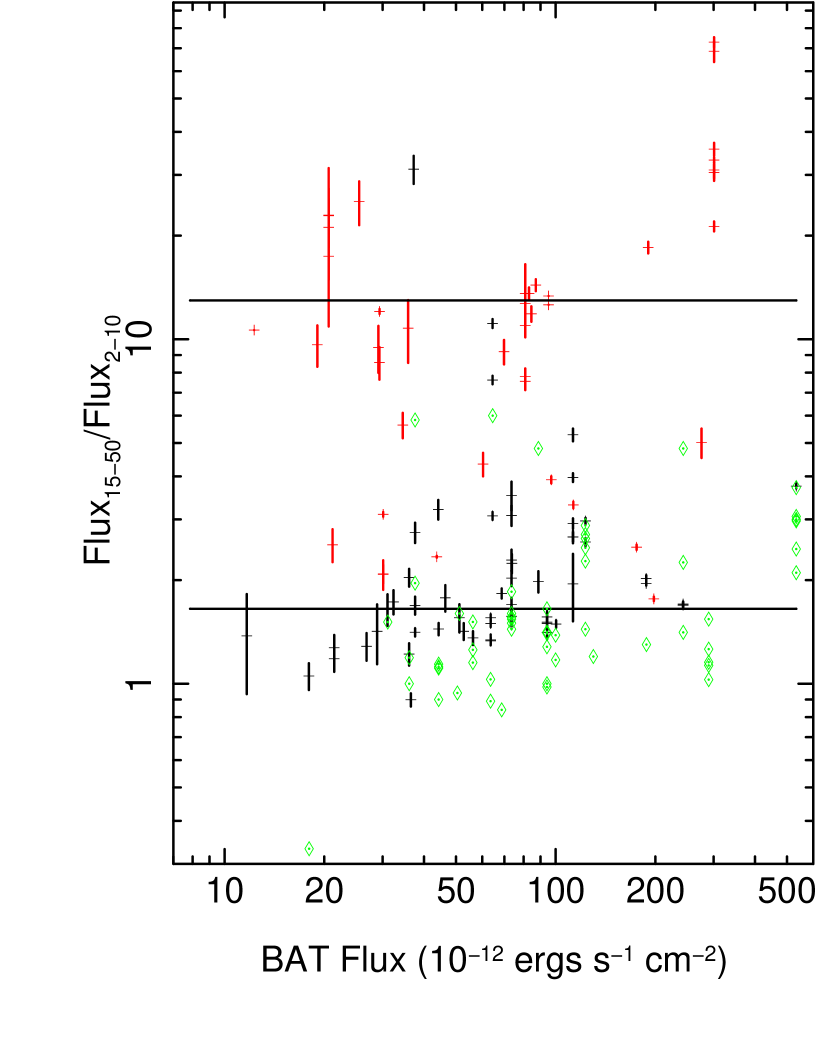
Figure 1: The hardness ratio, Flux${}_{15-50\,\textnormal{keV}}$/Flux${}_{2-10\,\textnormal{keV}}$, plotted against the Swift BAT flux, including both the type 1 (black markers) and type 2 (red markers) AGN observed using Suzaku. Overlaid are the hardness ratios we have extracted from the D07 sample points observed using BeppoSax (green). Solid lines represent the weighted hardness ratio mean of the type 1 (lower black line) and type 2 sources (upper black line) from the Suzaku sample analysis.

Following T13, for each observation in our sample, we plotted the Flux${}_{15-50\,\textnormal{keV}}$/Flux${}_{2-10\,\textnormal{keV}}$ against the BAT flux (Figure 1). The lower and upper solid black lines are the weighted mean Flux${}_{15-50\,\textnormal{keV}}$/Flux${}_{2-10\,\textnormal{keV}}$ for the type 1 ($1.73$) with variance 0.42 and type 2 AGNs ($10.02$) with variance 22.75, respectively. We found the weighted mean hardness ratios by fitting the type 1 and type 2 AGN datasets with a constant model line. The hardness ratio distribution of the type 2 AGN overlaps with the type 1 AGN distribution, suggesting a continuous distribution of spectral hardness across the AGN population (Figure 1).

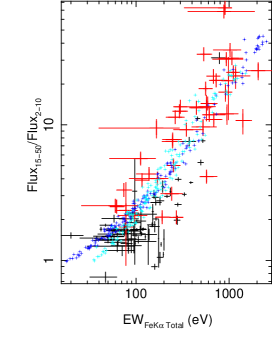
Figure 2: The hardness ratio plotted against the total Fe K$\alpha$ equivalent width, including both type 1 AGN (black markers) and type 2 AGN (red markers). Model overlaid are MCRT calculations assuming 1000 clouds in the spherical distribution, an inner radius of 10 units, an outer radius of 20 units, $\Gamma$=2.0, sin($\theta$) cloud distribution, and N_H = 9 x 10²³ (cyan crosses) and 2 x 10²⁴ cm^-2 (blue crosses).

T13 also plotted the Flux${}_{15-50\,\textnormal{keV}}$/Flux${}_{2-10\,\textnormal{keV}}$ against the EW of the total Fe K$\alpha$ emission line (measured against the total observed continuum). The addition of the type 2 AGN is shown in Figure 2, it reveals a continuous distribution of spectral hardness and line EW across the AGN population.

4.2 Comparison to BeppoSAX

It is instructive to compare the above results with those obtained previously from BeppoSAX observations. BeppoSAX (Boella et al., 1997) was the first X-ray mission to cover three orders of magnitude in energy (0.1–300 keV) and comprised the Medium Energy Concentrator Spectrometer and the Photoswich Detection System, covering the 1.3–10 keV and 15–300 keV bandpasses, respectively. The broad bandpass of BeppoSAX allowed for simultaneous soft, medium, and hard X-ray data.

Utilizing this broadband capability, Dadina (2007, hereafter D07) and Dadina (2008, hereafter D08) conducted an archival study of the Seyfert galaxies (type 1-1.9 and type 2) at z $\leq$ 0.1 observed with BeppoSAX. The sample overlaps our own, although we note that the selection criteria were different: D07 did not select the sources on hard X-ray flux and did allow inclusion of some radio-loud AGN. D07 fitted these sources with a template model consisting of a powerlaw, a gaussian component and a reflection component, with more complex components added when statistically required. During spectral fitting, D07 allowed the photon index to float, finding some relatively flat indices in the sample. D07 also allowed the Fe K$\alpha$ emission line and the reflection continuum to be modeled independently. D08 statistically analyzed the D07 results to understand the characteristics of the nearby Seyfert population and found R = 1.23 $\pm$ 0.11, suggesting that the hard excess phenomenon is not ubiquitous in AGN, in contrast to the results of Tatum et al. (2013).

To understand this discrepancy, we cross-correlated the T13 sample with the D07 sample and calculated the ratio Flux${}_{15-50\,\textnormal{keV}}$/Flux${}_{2-10\,\textnormal{keV}}$ for the overlapping sources and overlaid them on our Suzaku sample. The BeppoSAX data show very hard X-ray spectral forms for the D07 sample (Figure 1) with a mean hardness ratio 1.87. While our sample and that of D07 span the local AGN population, it is not surprising that our sample shows a greater number of hard sources, as our sample was hard X-ray selected.

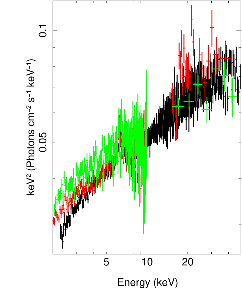
Figure 3: Spectra of the August 12, 2012 NuSTAR observation (black), the August 1, 2007 Suzaku observation (red) and the July 21, 1998 BeppoSAX observation (green) of IC4329A.

As a more stringent test of our hardness result we compared the IC4329A spectra from BeppoSAX (July 21, 1998), Suzaku (August 1, 2007) and NuSTAR (August 12, 2012) observations. NuSTAR is the first hard X-ray imaging telescope (FWHM angular resolution $\sim$ 17$\arcsec$), covering the 5-80 keV bandpass. The focusing optics and CZT detectors allow for low background rates and sensitivity two orders of magnitude better than previous hard X-ray missions (Harrison et al., 2010). As shown in Figure 3, the spectral shape is consistent among all the observations, showing the same result is obtained from all broad-band detectors.

If we apply the spectral models of D07 to our Suzaku spectra, we get broad agreement with D07. However, we believe our modeling approach is well justified. Large sample studies such as that of Scott et al. (2011) have found $\Gamma=1.99\pm 0.01$, in agreement with detailed analysis of high quality data for some well-studied objects (e.g. $\Gamma\sim$ 2.1 for MCG-06-30-15 Miller et al., 2008). Such an analysis involved inclusion of a complex, multi-zoned absorber into the spectral model. Continuum slopes around $\Gamma\sim 2$ are steeper than those fitted by D07, and if such an index was fixed in the D07 fits then the reflection contributions returned by the BeppoSAX data would necessarily be higher than those tabulated by D07. The D07 modeling approach returned not only flat photon indices, but also required the photon index to vary over a large range of values ($\Delta\Gamma\sim 0.3$) in some individual sources, on timescales of weeks to months. Such drastic changes in spectral shape within observations of an individual object may be explained better by variations in the absorber along the line of sight rather than large changes in the continuum form (e.g. Miller et al., 2008). We conclude that the lack of any strong hard components in the fit results from the D07 analysis is attributable to the different approach used for spectral fitting. We move forward by analyzing the data in the context of our preferred model.

5 Monte-Carlo Radiative Transfer Calculation

Our aim in this paper is to test whether we may explain the gross X-ray spectral properties of the local AGN population with a simple, but physically self-consistent, model of reprocessing by circumnuclear material. To this end we use a simple Monte-Carlo Radiative Transfer (MCRT) code, which was originally presented in T13. We present here a general overview and refer the reader to T13 for specific details.

The MCRT calculation presented in T13 uses a simple model of a partial covering atmosphere. At every point this atmosphere is assumed to be a strict two-phase medium which is either vacuum or cold, neutral gas at constant density. In reality the atmosphere is likely to be hot and ionized, however to explore a wide range of parameter space, the model presented here makes the simplifying assumption of cold gas clouds, such that all ions heavier than H are neutral, but with H ionized, so that the number of free scattering electrons equals the number of H atoms. An inhomogeneous model atmosphere is created by randomly placing a set of spherical gas clouds within a spherical annulus centered on the primary source, with the annulus having a defined inner and outer radius. The results are independent of any scale size for the cloud distribution, as all length scales are relative to an individual sphere’s radius. The probability density distribution from which these points are drawn is symmetric azimuthally, but may have some dependence on polar angle. If two (or more) spheres overlap, the density is not doubled, but remains at the same value as elsewhere in the gas phase. For distributions with a high density of points, the spheres heavily overlap, and the resulting gas distribution does not then resemble a set of individual blobs, but rather a sponge-like topology. It is assumed that the intrinsic X-ray continuum source is relatively compact and likely associated with an accretion disk corona. For the radiative transfer calculation, the spherical distribution is assumed to be bisected by an infinite, thin accretion disk, that absorbs photons but does not itself radiate at X-ray energies, so that the scattered light received by the observer is reduced by a factor two compared with the optically-thin case without the disk. The reason for setting the accretion disc as being a black absorber is to show that any results we obtain are due entirely to the cloud distribution. We might also expect some disc reflection, and more sophisticated modeling could include that. However, the main objective in using MCRT is not to carry out a detailed and realistic modeling of X-ray spectra, but rather to determine if a simple model that nonetheless has some self-consistent radiative transfer physics can explain the broad spectral properties of the entire AGN population.

As photons propagate through the distribution they may be either absorbed by the gas, or be Compton scattered. After absorption, there may be resulting Fe K fluorescent line emission. This is implemented by calculating the mean free path for the photon in the gas due to three processes:

1. Compton scattering, using the full energy-dependent Klein-Nishina cross-section, integrated over all scattering angles.

2. Absorption by elements other than K-shell transitions of Fe, in which case the photon disappears from the calculation (i.e. line emission from elements other than Fe K-shell transitions, primarily in the soft X-ray band, is neglected).

3. Absorption by an Fe K-shell transition, which may be followed by Fe K$\alpha$ or Fe K$\beta$ fluorescent line emission.

5.1 Modifications to MCRT

The MCRT code used in T13 generated spectra by summing the observed photons over a large number of sightlines, effectively producing a spectrum averaged over many sightlines for a given input atmosphere. However, one expects considerable variations between spectra generated for different sightlines within the same atmosphere, considering the highly inhomogeneous nature of this partial covering model, and in this paper we investigate whether the dispersion in the observed properties of AGN may be attributed to natural variation between differing sightlines. In order to sample the range of sightlines produced by a single atmosphere, this code was modified to generate spectra binned over a full range of both azimuthal and polar angles. Taken together, they covered the full 2$\pi$ sr. The hemisphere was divided into regions of equal solid angle, each covering a small range in both the polar angle ($\theta$) and azimuthal angle ($\phi$), and each corresponding to a potential observed sightline.

In each spectrum, an effective observed solid angle was determined by requiring it to be sufficiently large such that the majority of sightlines are partially covered and sufficiently small to produce variation between sightlines. In choosing the solid angle of a sightline, we effectively estimate the ratio between the characteristic size of the atmosphere and the size of the X-ray emitting region. We expect the scale of the source and the cloud structure might be similar (Turner & Miller, 2009); therefore, we divided the polar angle into bin sizes equaling the angle subtended by one radius at the inner edge of the spherical distribution, approximately 10^o. Each bin was then subdivided into azimuthal bins with the same size criterion.

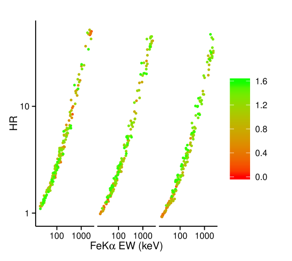
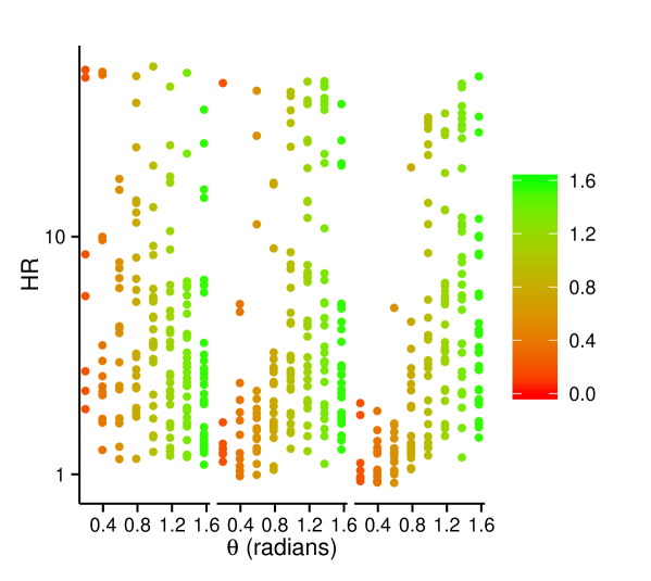
Figure 4: : MCRT simulated hardness ratio (HR) plotted against Fe K$\alpha$ equivalent width (EW) (top) and the MCRT simulated hardness ratio plotted against polar viewing angle ($\theta$) (bottom) with varying degrees of anisotropy. The spatial density of cloud centers is proportional to constant (left), sin$\theta$ (middle), and sin²$\theta$ (right), and the colors indicate the polar angle of a sightline in radians.

In order to investigate the effects of anisotropy in the AGN atmosphere, we further modified the code to allow the clouds to be placed with a spatial density that is either constant, proportional to sin($\theta$), or proportional to sin²($\theta$), allowing the potential for the cloud density to be preferentially aligned along the plane of the accretion disk. Figure 4 displays the results of three such simulations. Note that only the number of clouds per unit volume changed, while the density of the gas remained constant. The hardness ratio and equivalent width distribution has a dependence on geometry. The HR-EW relationship for constant cloud density is consistent with any polar viewing angle. However, as the cloud distribution becomes more anisotropic, the higher equivalent widths and hardness ratios correspond to larger polar viewing angles, i.e., more edge-on sightlines.

Note that the MCRT model results are invariant with respect to any choice of electron density or cloud size, these parameters may be subsumed into a single model parameter, which is the column density through the diameter of one cloud. The results are also invariant with respect to the size of overall the cloud distribution, for a given column density and cloud geometry, the whole distribution may be scaled up or down in size without affecting the resulting spectra.

6 Interpretation of the distribution of results in the hardness ratio - Fe K$\alpha$ plane

We compared our observational result with calculations from the modified MCRT code. The calculations in Figure 2 were performed assuming 1000 clouds in the spherical distribution, an inner radius of 10 units, an outer radius 20 units, $\Gamma$=2.0, a sin($\theta$) cloud distribution and N_H = 9 x 10²³ and 2 x 10²⁴ cm^-2. These simulations are consistent with the type 1 and type 2 spectral properties of our sample. In the N_H=2 x 10²⁴ cm^-2 simulation, 48% and 52% of sightlines were obscured by Compton-thick (N_H $>$ 10²⁴ cm^-2) and Compton-thin (N_H $<$ 10²⁴ cm^-2) columns of gas, respectively.

As shown in Figure 2, the modified MCRT model is capable of creating a distribution of spectra that follows the general trend visible in the observational data. However, in order to make a meaningful comparison between the two, we require a statistical procedure than can quantify the similarity between the two distributions. In this case, we used the 1D Kolmogorov-Smirnoff (KS) test and treated the MCRT model as the probability distribution and the observational data as the sample.

A useful feature of the KS test is that the distribution of the test statistic is independent of the probability distribution function being tested. This allows us to perform it relatively easily, without needing to determine what the distribution of the test statistic should be for each set of model results individually. A disadvantage of the test, however, is that the statistical significance of the test statistic is unknown if model parameters are varied. In this paper, our aim is not to carry out a full statistical test of goodness-of-fit, as the model is certainly too simplistic, in that it assumes that every AGN in the sample has an identical distribution of circumnuclear gas, with only the line of sight to the nucleus differing between AGN. Hence we use the KS test only as indicative of the relative success of our choice of basic models. We performed two 1D KS tests, treating the EW and HR independently of each other. Although this approach loses information about the correlation in the data, it remains helpful as an indicator of goodness of fit. Before the model could be tested against the data, it was important to consider the experimental errors present in the observations. These errors are vastly greater than the Monte Carlo noise in the MCRT model spectra. If the model were a good description of the X-ray spectra of AGN, we would expect to observe that distribution of spectra blurred by considerable experimental errors. To meaningfully compare model and observation, we must generate the distribution of HRs and EWs that we would expect to recover with our instruments if we were to observe the spectra generated by the MCRT model. Therefore, before any KS tests were performed it was necessary to add simulated experimental errors to the model’s predictions.

One way to generate simulated experimental errors is to make use of the errors present in the observational data. Because we are treating the EW and HR as independent for the purposes of our statistical tests, a reasonable way to generate an error for the EW of a model point is to select the n closest observational data points along the EW axis and assign the model point a standard error equal to the average of the standard errors on those n data points, likewise for the HR. A blurred model distribution can then be produced by randomly generating a number of new points for each model point, with the new points drawn from a normal distribution centered on the original model point and with a standard deviation equal to the error which we have assigned to that point.

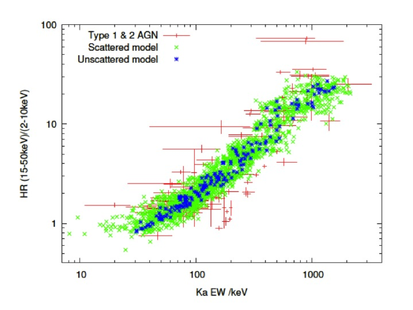
Figure 5: A subset of the MCRT model predictions with (green) and without (blue) error-scatter overlay the equivalent width distribution of the type 1 and type 2 AGN (red). The models assumed N_H = $10^{24}$ cm^-2, $\Gamma$ = 2.1 and outer radius=20 cloud radii.

In order to carry out the blurring with simulated experimental errors and the pair of KS tests, we generated 1000 scattered points for each original model point, with errors derived by averaging those of the nearest 10 observational data points in logarithmic space. This resulted in error-scattered distributions with low Monte Carlo noise, which reduced to approximately continuous cumulative density functions along both EW and HR axes (a requirement of the KS testing process). We then performed a pair of 1D KS tests treating the two variables as independent. An example of a model distribution which has been scattered in this way can be seen in Figure 5.

The results of performing the KS tests were dependent on the assumed input parameters, with particularly high dependence on the column density per cloud (N_H). We obtained the highest p-values, p_EW = 0.75 and p_HR = 0.046 for the EW and HR 1D KS tests, assuming N_H = 10²⁴ cm^-2, $\Gamma$ = 2.1, cloud density distribution proportional to sin$\theta$, and outer radius= 20 cloud radii.

With values of up to 0.75 for p_EW, the MCRT model appears to generate a very similar distribution of EWs to that observed in both type 1 and type 2 Seyfert galaxies. Examination of Figures 2 and  5 shows the model predictions include a tail of very low hardness ratios that represent the least obscured sight-lines, where a direct view to the source results in no absorption of soft X-rays and hence no excess hardness in the spectrum. Indeed, several so-called ’bare’ Seyfert galaxies have been reported in the literature (e.g. Ark 120 and Fairall-9, Patrick et al. 2011). Overall, the distribution of simulated spectra and those in our observed population are consistent, suggests that partial covering atmospheres of Compton thick gas may play an important part in the unified model of AGN X-ray spectra.

7 X-ray Luminosity Correlation

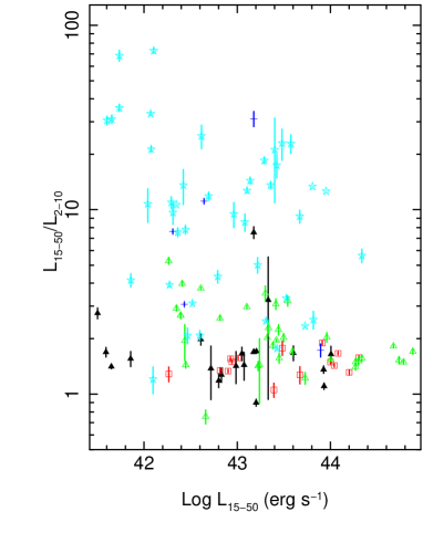
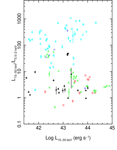
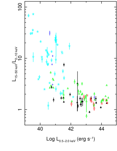
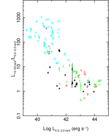
Figure 6: Top: the 15-50/2-10 keV luminosity ratio (left) and 15-50/0.5-2 keV luminosity ratio (right) plotted against the 15-50 keV luminosity. Bottom: the 15-50/2-10 keV luminosity ratio (left) and 15-50/0.5-2 keV luminosity ratio (right) plotted against the 0.5-2 keV luminosity. With type 1 (filled black triangles), type 1.2 (red squares), type 1.5 (open green triangles), type 1.8-1.9 (dark blue crosses) and type 2 AGN (aqua stars).

Next we investigated the relationship between the luminosities in different X-ray bands, with the goal of improving our understanding of the reprocessor. Figure 6 shows the 15–50 keV / 2-10 keV luminosity ratio and the 15-50/0.5-2 keV luminosity ratio plotted against both the 15-50 keV luminosity and 0.5-2 keV luminosity. It is evident (top panels) that the type 2 AGN have the same hard-band (15-50 keV) luminosity distribution as the rest of the AGN population. This supports the expectation, from Unified Models, that the different optical classes should harbor nuclei of the same power. The uniformity of luminosity distributions for type 1 and type 2 AGN is indicative that the 15-50 keV luminosity is a fair representation of the true intrinsic continuum luminosity.

It is also clear that the type 2 AGN (aqua stars) have systematically lower soft-band luminosities than the rest of the population (lower panels): this is already well known and thought to be due to the relatively high obscuration of the primary continuum for type 2 AGN versus type 1 AGN in this soft energy band (Halderson et al., 2001). A few intermediate type AGN appear at low soft-band luminosities, as expected from our cloud model, where the obscuration is a probability function across the AGN optical types and also varies with time for an individual object.

The type 2 AGN show a broader distribution of hardness ratios relative to type 1 sources, again, consistent with our view that the absorber is clumpy and has a polar angle dependence for the cloud distribution. Type 2 AGN are viewed through the largest number of clouds (‘edge-on to the distribution’) and can therefore produce the hardest spectra. However, the Type 2’s also have the greatest potential to exhibit a large range of hardness, as these clouds move in and out of the line-of-sight.

8 Discussion

We have extended the work of T13 to consider the broad properties of a hard X-ray selected set of local AGN, thought to provide an unbiased representation of the local population. The consistency of the luminosity distributions of type 1 and type 2 AGN in the 15-50 keV band indicates that this band does indeed provide a relatively unbiased selection criterion. The spectral hardness and Fe K$\alpha$ have once again been used as a diagnostic of the reprocessing gas. Extending the results of T13, we have found that the local radio-quiet AGN population yields a continuous distribution of values for spectral hardness and line equivalent width. A detailed comparison shows that our Suzaku results are consistent with measurements across a similar bandpass from previous observations using BeppoSAX.

The range of X-ray spectral properties exhibited across the population can be parameterized within the context of a simple circumnuclear cloud model, calculated here using Monte Carlo radiative transfer techniques. As proof of the concept, we have fitted the sample with a model atmosphere that has a column density $N_{H}=10^{24}{\rm atoms\,cm^{-2}}$ with inner and outer radii for the shell set at 10 and 20 cloud radii, and using 1000 clouds filling our shell with a sin$\theta$ dependence of the cloud density on polar angle. The range of observed AGN types are then explained primarily by different sight-lines through the cloud ensemble to the nucleus. This shows that the obscuring material required by unified theories may be related to the X-ray absorber seen in type 1 AGN, as previously suggested from X-ray studies (e.g. Cappi et al., 2000).

There is significant short-timescale variability in the X-ray absorption of both type 1 and type 2 AGN (e.g., Turner et al., 2000; Miller et al., 2008; Risaliti et al., 2010, and references therein), which, in the most extreme cases produces a so-called ‘changing look’ AGN (e.g. Matt et al., 2003; Braito et al., 2014). A clumpy X-ray absorber is required to explain the observed X-ray absorption variability of AGN, as also suggested by Markowitz et al. (e.g 2014). The characteristic variability timescales coupled with the result of this work supports previous suggestions that the X-ray absorber is part of a massive outflow, whose presence is observed across a broad bandpass in energy (e.g., Elitzur & Shlosman, 2006; Elitzur, 2008). The clumpy nature of the torus is not only evidenced from X-ray observations, but has also been suggested based on theoretical models to explain the isotropic infrared emission coupled with the anisotropic obscuration of AGN (e.g. Nenkova et al., 2008).

Ricci et al. (2014) studied the relationship between the narrow Fe K$\alpha$ emission line and the 10-50 keV continuum in Seyfert 1 and 2s and found the L_FeKα/L${}_{10-50\,\textnormal{keV}}$ is lower on average in Seyfert 2s than Seyfert 1s, consistent with the idea that the Fe K line emission may be self-absorbed by the reprocessor in type 2 objects, which is evident in our MCRT model results.

In the context of MCRT, T13 estimated the location of the Compton-thick, X-ray absorber to be within the optical broad line region. Shu et al. (2011, hereafter S11) studied the Fe K alpha emission cores of 10 type 2 AGN (4 of which are included in our study) and compared them to the Fe K alpha emission core of 13 type 1 AGN. They found a marginal difference between the Fe K alpha luminosity in type 1 and type 2 AGN and concluded the Fe K alpha emitting region for the type 2 AGN lies between the outer part of the optical broad line region and the putative torus.

9 Conclusions

Using the 58-month BAT catalog, we have identified and analyzed an unbiased sample of Suzaku observations representative of the local population of radio-quiet AGN. We have demonstrated how a single, simple cloud reprocessing ensemble can explain the gross sample properties across all AGN types.

Examination of the spectral hardness and Fe K$\alpha$ equivalent width shows a continuous distribution of properties from type 1 to type 2 AGN. Comparison of the data with our Monte Carlo Radiative Transfer model for a reprocessing cloud ensemble shows the local population of radio-quiet AGN is consistent with reprocessing of the X-ray continuum in an ensemble of low-ionization, Compton-thick clouds. This cloud distribution allows us to reproduce the entire range of observed properties simply by changing the observer’s sightline. Of course, other cloud variations across the sample ($\xi$, N_H etc) are expected, but the primary cause of the correlated variation in hardness ratio and line equivalent width for the entire sample of type 1 and type 2 AGN may be ascribed simply to differing lines of sight through a clumpy circumnuclear distribution of absorbing and Compton scattering gas.

Such an X-ray absorber would likely form part of a clumpy, massive outflow, that would shape the broad observed spectral shape of the AGN, and would form an important component of material and energetic feedback between the galaxy nucleus and the host.

Table 1: X-ray Observation Type 2 Source List

Object	ObsID	RA (h m s)	Dec (∘ ′  ″)	z	NH(Gal)	Type	Hardness Ratio	Total EW (eV)
NGC 4138	704047010	12 09 29.8	+ 43 41 07	0.003	0.014	1.9	2.19 $\pm{0.40}$	151 ${}^{+15}_{-75}$
2MASXJ02485937+2630391	704013010	02 48 59.3	+ 26 30 39	0.058	0.104	2	5.64 $\pm{0.48}$	112 ${}^{+50}_{-60}$
2MASXJ04440903+2813003	703021010	04 44 09.0	+ 28 13 01	0.011	0.196	2	4.34 $\pm{0.34}$	138 ${}^{+14}_{-37}$
2MASXJ12005792+0648226	703009010	12 00 57.9	+ 06 48 23	0.036	0.014	2	2.53 $\pm{0.28}$	60 ${}^{+48}_{-34}$
2MASXJ20183871+4041003	506018010	20 18 38.7	+ 40 41 00	0.014	1.200	2	8.56 $\pm{0.93}$	65 ${}^{+71}_{-44}$
Ark347	705002010	12 04 29.7	+ 20 18 58	0.022	0.024	2	9.47 $\pm{1.47}$	166 ${}^{+126}_{-126}$
ESO005-G004	701018010	06 05 41.6	– 86 37 55	0.006	0.111	2	10.77 $\pm{2.23}$	1407 ${}^{+341}_{-221}$
ESO103-G035	703031010	18 38 20.3	– 65 25 39	0.013	0.076	2	3.31 $\pm{0.07}$	74 ${}^{+16}_{-12}$
ESO137-G034	403075010	16 35 14.1	– 58 04 48	0.009	0.247	2	1.20 $\pm{0.20}$	950 ${}^{+300}_{-250}$
ESO 297-018	701015010	01 83 37.1	– 40 00 41	0.025	0.020	2	11.38 $\pm{0.30}$	264 ${}^{+66}_{-53}$
IGRJ12391-1612	703007010	12 39 06.3	– 16 10 47	0.037	0.037	2	2.34 $\pm{0.01}$	78 ${}^{+26}_{-17}$
MCG+4-48-002	702081010	20 20 35.0	+ 25 44 00	0.014	0.260	2	12.69 $\pm{0.34}$	648 ${}^{+122}_{-73}$
MCG -01-05-047	704043010	01 52 49.0	– 03 26 49	0.017	0.025	2	4.01 $\pm{0.10}$	170 ${}^{+51}_{-85}$
MCG -02-08-014	704045010	02 52 23.4	– 08 30 37	0.017	0.046	2	2.14 $\pm{0.02}$	97 ${}^{+34}_{-33}$
MCG-5-23-16	700002010	09 47 40.1	– 30 56 55	0.008	0.080	2	1.76 $\pm{0.03}$	78 ${}^{+6}_{-7}$
Mrk18	705001010	09 01 58.4	+ 60 09 06	0.011	0.044	2	10.64 $\pm{0.01}$	253 ${}^{+129}_{-100}$
NGC1068	701039010	20 42 40.7	– 00 00 48	0.004	0.035	2	4.15 $\pm{0.35}$	573 ${}^{+169}_{-71}$
NGC1142	701013010	02 55 12.2	– 00 11 01	0.029	0.064	2	12.59 $\pm{0.00}$	293 ${}^{+65}_{-22}$
NGC1142	702079010	02 55 12.2	– 00 11 01	0.029	0.064	2	13.36 $\pm{0.00}$	445 ${}^{+193}_{-54}$
NGC2992	700005010	09 45 42.0	– 14 19 35	0.008	0.053	2	2.08 $\pm{0.20}$	271 ${}^{+49}_{-19}$
NGC2992	700005020	09 45 42.0	– 14 19 35	0.008	0.053	2	2.08 $\pm{0.13}$	191 ${}^{+43}_{-26}$
NGC2992	700005030	09 45 42.0	– 14 19 35	0.008	0.053	2	3.10 $\pm{0.05}$	242 ${}^{+74}_{-57}$
NGC3081	703013010	09 59 29.5	– 22 49 35	0.008	0.046	2	11.86 $\pm{0.62}$	612 ${}^{+296}_{-75}$
NGC3281	703033010	10 31 52.1	– 34 51 13	0.011	0.064	2	14.37 $\pm{0.58}$	589 ${}^{+156}_{-66}$
NGC3393	702004010	10 48 23.4	– 25 09 43	0.013	0.061	2	25.09 $\pm{3.65}$	2059 ${}^{+1227}_{-477}$
NGC4388	800017010	12 25 46.7	+ 12 39 44	0.008	0.026	2	5.01 $\pm{0.49}$	253 ${}^{+11}_{-10}$
NGC4507	702048010	12 35 36.6	– 39 54 33	0.012	0.072	2	18.48 $\pm{0.72}$	560 ${}^{+28}_{-30}$
NGC454	704009010	01 14 22.5	– 55 23 55	0.012	0.027	2	9.65 $\pm{1.33}$	525 ${}^{+205}_{-126}$
NGC4945	100008010	13 05 27.5	– 49 28 06	0.002	0.157	2	21.27 $\pm{0.70}$	727 ${}^{+228}_{-82}$
NGC4945	100008030	13 05 27.5	– 49 28 06	0.002	0.157	2	33.14 $\pm{0.62}$	534 ${}^{+117}_{-41}$
NGC4945	705047010	13 05 27.5	– 49 28 06	0.002	0.157	2	68.55 $\pm{4.76}$	882 ${}^{+996}_{-520}$
NGC4945	705047020	13 05 27.5	– 49 28 06	0.002	0.157	2	35.64 $\pm{1.55}$	1024 ${}^{+313}_{-344}$
NGC4945	705047030	13 05 27.5	– 49 28 06	0.002	0.157	2	72.87 $\pm{2.47}$	907 ${}^{+153}_{-576}$
NGC4945	705047040	13 05 27.5	– 49 28 06	0.002	0.157	2	31.00 $\pm{1.65}$	1072 ${}^{+334}_{-306}$
NGC4945	705047050	13 05 27.5	– 49 28 06	0.002	0.157	2	30.50 $\pm{1.68}$	933 ${}^{+475}_{-266}$
NGC 5728	701079010	14 42 23.9	– 17 15 11	0.009	0.078	2	24.37 $\pm{0.40}$	1110 ${}^{+111}_{-111}$
NGC6300	702049010	17 16 59.5	– 62 49 14	0.004	0.099	2	3.91 $\pm{0.09}$	116 ${}^{+14}_{-18}$
NGC6552	504070010	18 00 07.3	+ 66 36 54	0.026	0.042	2	22.94 $\pm{4.43}$	1176 ${}^{+502}_{-141}$
NGC6552	504072010	18 00 07.3	+ 66 36 54	0.026	0.042	2	22.85 $\pm{2.67}$	679 ${}^{+0}_{-0}$
NGC6552	504074010	18 00 07.3	+ 66 36 54	0.026	0.042	2	17.43 $\pm{2.52}$	913 ${}^{+0}_{-0}$
NGC6552	504076010	18 00 07.3	+ 66 36 54	0.026	0.042	2	21.15 $\pm{10.25}$	984 ${}^{+0}_{-0}$
NGC7172	703030010	22 02 01.9	– 31 52 11	0.009	0.017	2	2.49 $\pm{0.04}$	62 ${}^{+13}_{-9}$
NGC7582	702052010	23 18 23.5	– 42 22 14	0.005	0.019	2	7.80 $\pm{0.43}$	248 ${}^{+60}_{-55}$
NGC7582	702052020	23 18 23.5	– 42 22 14	0.005	0.019	2	7.55 $\pm{0.43}$	247 ${}^{+65}_{-56}$
NGC7582	702052030	23 18 23.5	– 42 22 14	0.005	0.019	2	13.59 $\pm{2.92}$	571 ${}^{+142}_{-102}$
NGC7582	702052040	23 18 23.5	– 42 22 14	0.005	0.019	2	10.95 $\pm{0.83}$	686 ${}^{+154}_{-124}$
NGC788	703032010	02 01 06.4	– 06 48 56	0.014	0.022	2	13.58 $\pm{0.55}$	299 ${}^{+169}_{-38}$
SWIFTJ0138.6-4001	701015010	01 38 37.1	– 40 00 41	0.025	0.020	2	9.20 $\pm{0.75}$	347 ${}^{+184}_{-93}$

References

- Baumgartner et al. (2010) Baumgartner, W. H., Tueller, J., Markwardt, C., & Skinner, G. 2010, in Bulletin of the American Astronomical Society, Vol. 42, AAS/High Energy Astrophysics Division #11, 675
- Boella et al. (1997) Boella, G., Butler, R. C., Perola, G. C., Piro, L., Scarsi, L., & Bleeker, J. A. M. 1997, A&AS, 122, 299
- Boldt (1987) Boldt, E. 1987, in IAU Symposium, Vol. 124, Observational Cosmology, ed. A. Hewitt, G. Burbidge, & L. Z. Fang, 611–615
- Braito et al. (2014) Braito, V., Reeves, J. N., Gofford, J., Nardini, E., Porquet, D., & Risaliti, G. 2014, ApJ, 795, 87
- Cappi et al. (2000) Cappi, M., Bassani, L., Malaguti, G., Palumbo, G. G. C., Dadina, M., Comastri, A., Di Cocco, G., Blanco, P., dal Fiume, D., Fabian, A., Frontera, F., Guainazzi, M., Maccacaro, T., Maiolino, R., Matt, G., Piro, L., Trifoglio, M., & Zhang, N. 2000, Advances in Space Research, 25, 815
- Crenshaw et al. (2003) Crenshaw, D. M., Kraemer, S. B., & George, I. M. 2003, ARA&A, 41, 117
- Dadina (2007) Dadina, M. 2007, A&A, 461, 1209
- Dadina (2008) —. 2008, A&A, 485, 417
- Dickey & Lockman (1990) Dickey, J. M. & Lockman, F. J. 1990, ARA&A, 28, 215
- Elitzur (2008) Elitzur, M. 2008, Nature, 52, 274
- Elitzur & Shlosman (2006) Elitzur, M. & Shlosman, I. 2006, ApJ, 648, L101
- Fabian (1994) Fabian, A. C. 1994, ApJS, 92, 555
- Gofford et al. (2013) Gofford, J., Reeves, J. N., Tombesi, F., Braito, V., Turner, T. J., Miller, L., & Cappi, M. 2013, MNRAS, 430, 60
- Halderson et al. (2001) Halderson, E. L., Moran, E. C., Filippenko, A. V., & Ho, L. C. 2001, AJ, 122, 637
- Harrison et al. (2010) Harrison, F. A., Boggs, S., Christensen, F., Craig, W., Hailey, C., Stern, D., Zhang, W., Angelini, L., An, H., Bhalerao, V., Brejnholt, N., Cominsky, L., Cook, W. R., Doll, M., Giommi, P., Grefenstette, B., Hornstrup, A., Kaspi, V., Kim, Y., Kitaguchi, T., Koglin, J., Liebe, C. C., Madejski, G., Kruse Madsen, K., Mao, P., Meier, D., Miyasaka, H., Mori, K., Perri, M., Pivovaroff, M., Puccetti, S., Rana, V., & Zoglauer, A. 2010, in Society of Photo-Optical Instrumentation Engineers (SPIE) Conference Series, Vol. 7732, Society of Photo-Optical Instrumentation Engineers (SPIE) Conference Series
- Kaspi et al. (2002) Kaspi, S., Brandt, W. N., George, I. M., Netzer, H., Crenshaw, D. M., Gabel, J. R., Hamann, F. W., Kaiser, M. E., Koratkar, A., Kraemer, S. B., Kriss, G. A., Mathur, S., Mushotzky, R. F., Nandra, K., Peterson, B. M., Shields, J. C., Turner, T. J., & Zheng, W. 2002, ApJ, 574, 643
- Lohfink et al. (2012) Lohfink, A. M., Reynolds, C. S., Miller, J. M., Brenneman, L. W., Mushotzky, R. F., Nowak, M. A., & Fabian, A. C. 2012, ApJ, 758, 67
- Maeda et al. (2008) Maeda, Y., Someya, K., Ishida, M., the XRT team, Hayashida, K., Mori, H., & the XIS team. 2008, JX-ISAS-SUZAKU-MEMO-2008-06
- Markowitz et al. (2014) Markowitz, A. G., Krumpe, M., & Nikutta, R. 2014, MNRAS, 439, 1403
- Matt et al. (2003) Matt, G., Guainazzi, M., & Maiolino, R. 2003, MNRAS, 342, 422
- Miller & Turner (2013) Miller, L. & Turner, T. J. 2013, ApJ, 773, L5
- Miller et al. (2008) Miller, L., Turner, T. J., & Reeves, J. N. 2008, A&A, 483, 437
- Miller et al. (2007) Miller, L., Turner, T. J., Reeves, J. N., George, I. M., Kraemer, S. B., & Wingert, B. 2007, A&A, 463, 131
- Nenkova et al. (2008) Nenkova, M., Sirocky, M. M., Nikutta, R., Ivezić, Ž., & Elitzur, M. 2008, ApJ, 685, 160
- Patrick et al. (2011) Patrick, A. R., Reeves, J. N., Porquet, D., Markowitz, A. G., Lobban, A. P., & Terashima, Y. 2011, MNRAS, 411, 2353
- Pounds et al. (2003) Pounds, K. A., Reeves, J. N., King, A. R., Page, K. L., O’Brien, P. T., & Turner, M. J. L. 2003, MNRAS, 345, 705
- Rees (1977) Rees, M. J. 1977, QJRAS, 18, 429
- Reeves et al. (2009) Reeves, J. N., O’Brien, P. T., Braito, V., Behar, E., Miller, L., Turner, T. J., Fabian, A. C., Kaspi, S., Mushotzky, R., & Ward, M. 2009, ApJ, 701, 493
- Ricci et al. (2014) Ricci, C., Ueda, Y., Paltani, S., Ichikawa, K., Gandhi, P., & Awaki, H. 2014, MNRAS, 441, 3622
- Risaliti et al. (2009) Risaliti, G., Braito, V., Laparola, V., Bianchi, S., Elvis, M., Fabbiano, G., Maiolino, R., Matt, G., Reeves, J., Salvati, M., & Wang, J. 2009, ApJ, 705, L1
- Risaliti et al. (2010) Risaliti, G., Elvis, M., Bianchi, S., & Matt, G. 2010, MNRAS, 406, L20
- Risaliti et al. (2013) Risaliti, G., Harrison, F. A., Madsen, K. K., Walton, D. J., Boggs, S. E., Christensen, F. E., Craig, W. W., Grefenstette, B. W., Hailey, C. J., Nardini, E., Stern, D., & Zhang, W. W. 2013, Nature, 494, 449
- Scott et al. (2011) Scott, A. E., Stewart, G. C., Mateos, S., Alexander, D. M., Hutton, S., & Ward, M. J. 2011, MNRAS, 417, 992
- Shu et al. (2011) Shu, X. W., Yaqoob, T., & Wang, J. X. 2011, ApJ, 738, 147
- Tatum et al. (2013) Tatum, M. M., Turner, T. J., Miller, L., & Reeves, J. N. 2013, ApJ, 762, 80
- Tatum et al. (2012) Tatum, M. M., Turner, T. J., Sim, S. A., Miller, L., Reeves, J. N., Patrick, A. R., & Long, K. S. 2012, ApJ, 752, 94
- Terashima et al. (2009) Terashima, Y., Gallo, L. C., Inoue, H., Markowitz, A. G., Reeves, J. N., Anabuki, N., Fabian, A. C., Griffiths, R. E., Hayashida, K., Itoh, T., Kokubun, N., Kubota, A., Miniutti, G., Takahashi, T., Yamauchi, M., & Yonetoku, D. 2009, PASJ, 61, 299
- Tombesi et al. (2010) Tombesi, F., Cappi, M., Reeves, J. N., Palumbo, G. G. C., Yaqoob, T., Braito, V., & Dadina, M. 2010, A&A, 521, A57
- Turner & Miller (2009) Turner, T. J. & Miller, L. 2009, A&A Rev., 17, 47
- Turner et al. (2009) Turner, T. J., Miller, L., Kraemer, S. B., Reeves, J. N., & Pounds, K. A. 2009, ApJ, 698, 99
- Turner et al. (2000) Turner, T. J., Perola, G. C., Fiore, F., Matt, G., George, I. M., Piro, L., & Bassani, L. 2000, ApJ, 531, 245
- Turner et al. (2008) Turner, T. J., Reeves, J. N., Kraemer, S. B., & Miller, L. 2008, A&A, 483, 161
- Véron-Cetty & Véron (2006) Véron-Cetty, M.-P. & Véron, P. 2006, A&A, 455, 773
- Wilms et al. (2000) Wilms, J., Allen, A., & McCray, R. 2000, ApJ, 542, 914