Efficient MCMC implementation of multi-state mark-recapture models

Inherent differences in behaviour of individual animal movement can introduce bias into estimates of population parameters derived from mark-recapture data. Additionally, quantifying individual heterogeneity is of considerable interest in it’s own right as numerous studies have shown how heterogeneity can drive population dynamics. In this paper we incorporate multiple measures of individual heterogeneity into a multi-state mark-recapture model, using a Beta-Binomial Gibbs sampler using MCMC estimation. We also present a novel Independent Metropolis-Hastings sampler which allows for efficient updating of the hyper-parameters which cannot be updated using Gibbs sampling. We tested the model using simulation studies and applied the model to mark-resight data of North Atlantic humpback whales observed in the Stellwagen Bank National Marine Sanctuary where heterogeneity is present in both sighting probability and site preference. Simulation studies show asymptotic convergence of the posterior distribution for each of the hyper-parameters to true parameter values. In application to humpback whales individual heterogeneity is evident in sighting probability and propensity to use the marine sanctuary.

Keywords: Individual heterogeneity; Beta-binomial; Gibbs sampler; Independent Metropolis-Hastings sampler; MCMC; hidden Markov model; mark-recapture; North Atlantic humpback whales.

1 Introduction

Mark-recapture analysis is a fundamental tool for understanding populations. Demographic parameters estimated from mark-recapture data, such as survival and reproduction, are used to infer population status and predict future dynamics of population. Standard statistical techniques for estimating population parameters from mark-recapture data, often by omission, implicitly assume animals to be identical. This is something shared with most ecological models which assume populations to be composed of identical average individuals (Grimm and Uchmanski, 2002). While this is a convenient and often necessary simplification, individuals in wild populations typically do not behave, grow or reproduce identically. Neither are they identically observed by researchers (Crespin et al., 2008). This heterogeneity between individuals presents a challenge both for the collection and analysis of mark-recapture data. Individuals in natural populations tend to exhibit substantial individual variation which can manifest through demographic parameters (Lebreton et al., 1992). For example, inherent individual differences in movement and behavior can introduce bias into mark-recapture-derived estimates; most notoriously for inferring population size (Pledger et al., 2010). Moreover characterizing the extent of individual variability in some aspect of individuals biology is often of considerable interest in it’s own right as it can have substantial impact on population (Franklin et al., 2000) and even ecosystem dynamics (Vieilledent et al., 2010).

While mark-recapture analysis methods capable of explicitly including individual heterogeneity are not the norm, several studies have addressed the problem. Pledger (2000) and Norris and Pollock (1996) developed finite mixture models which assume that differences between individuals can be explained by categorising into a finite set of latent groups. Despite the computational advantage over other methods such as continuous random effects (Ford et al., 2012), this approach relies on the assumption of a prespecified number of groups and can result in model selection issues such as determining the number of groups of individuals sharing the same survival or detection parameter (Cubaynes et al., 2012).

Individual-level random effects using continuous distributions are a natural candidate for modelling heterogeneity as they do not require that individuals be categorized into prespecified groups. Random effects are useful as they can allow a proportion of variance on some population parameter (i.e. detection) to be related to persistent unobserved individual heterogeneity. In this context random effects allow individuals to obtain their own instance of a population parameter (e.g. detection probability), drawn from a common distribution whose parameters are estimated. However, despite inclusion of random effects being the focus of much research (Maunder et al., 2008; Lebreton et al., 2009; Barry et al., 2003; Royle and Dorazio, 2008; Huggins and Yip, 2001; Burnham and Overton, 1978; Gimenez and Choquet, 2010), methods for the inclusion of multiple individual-level continuous random effects into mark-recapture models are still lacking. This is in part due to the complex calculation required to solve for these random effects.

To estimate random effects models it is necessary to integrate across all possible values of the individual-level random effects which is not straightforward. Ford et al. (2012) provide one solution using the open source software Automatic Differentiation Model Builder with Random Effects (ADMB-RE, Fournier et al. 2012). Another possible technique is the use of Markov chain Monte Carlo (MCMC) as this provides a solution to the calculation of marginal distributions which involve complex integrals (Gilks et al., 1996).

One method to capture heterogeneity is through the development of multi-state mark-recapture models. Multi-state mark-recapture models, first developed by Arnason (Arnason, 1972, 1973), extend traditional mark-recapture models by allowing animals to be in different ‘states’ (Lebreton et al., 2009). The ’movement’ parameter, the probability of transitioning between states, was originally introduced to distinguish between emigration and mortality. The states, which may or may not be directly observable, can include, but are not limited, to breeding, location, and behaviour. State can affect the probability of observation, and this can be built into the multi-state framework (Lebreton and Pradel, 2002). These models can be extended (Pradel, 2005) through the use of a hidden Markov model framework, which incorporate a more realistic assessment of natural events as transitions between states can be treated as a Markov process that is not directly observable (Conn and Cooch, 2009; Zucchini et al., 2008). In hidden Markov models, two time series - the observation and process components - run in parallel (Gimenez et al., 2012). The observation process (e.g. seen/not seen) does not usually reveal the current underlying state directly, but does provide indirect information on the probable state (e.g. present in the marine sanctuary, not present, or dead). Modelling both the process and observation component enables the separation of the real signal from the observation error (Patterson et al., 2008).

Here we develop a multi-state model using a hidden Markov model framework which explicitly includes individual heterogeneity in sighting probability and site fidelity, and we apply it to a long term data set of North Atlantic humpback whales at the Stellwagen Bank National Marine Sanctuary (SBNMS) off the northeast coast of the United States. Individual humpback whales have been intensively studied in this region since the late 1970s. However, the SBNMS covers only a small part of the population’s summer range, and although some individuals are seen regularly there, none are thought to remain permanently within its boundaries. This presents a challenge when studying the vital rates of whales using the area and the effectiveness of management initiatives.

There are presently over 500 marine protected areas (MPAs) primarily for marine mammals. Declines in marine mammal populations have been attributed to a variety of factors: entanglement in fishing gear (Hoyt, 2011; Johnson et al., 2005; D’Agrosa et al., 2000), over fishing (Read et al., 2006), pollution (Wilgart, 2007), and ship strikes (Laist et al., 2001; Knowlton and Kraus, 2001). As these threats are often concentrated in space, MPAs have been advocated as an effective management strategy for mitigation. Determining the effectiveness of a MPA’s spatial configuration (e.g. location, extent) is challenging. An often overlooked factor is how individual heterogeneity in spatial use can mediate the effectiveness of a MPA.

Heterogeneity in sighting probability is a well known phenomenon (Hammond, 1986, 1990) as the probability of sighting relies on individual behaviour at the beginning of a dive. The angle to which an individual’s fluke shows on diving determines the probability of a successful photograph. The probability of being seen and recognized is therefore a combination of the true observation error (e.g. the randomness in viewing flukes) and also the real biological signal arising from individual heterogeneity in presence and absence in the SBNMS. The difficulty lies in determining the underlying behaviour of the whales: observations are indications of presence in the SBNMS but whales may also be present and not observed.

In this paper we develop a Bayesian hierarchical approach to incorporating random effects into a hidden Markov model using MCMC estimation. Following work by Zucchini et al. (2008) and Scott (2002) we develop a Beta-Binomial Gibbs sampler for the hidden Markov model. We also present a novel Independent Metropolis-Hastings sampler which allows efficient updating of the hyper-parameters which cannot be updated using Gibbs sampling. We employ a hidden Markov model which allows for individual variability on the probability of observation and the probability of remaining in either of the two states: resident in the SBNMS or elsewhere (see Ford et al., 2012). A two-state model is used for simulation testing and we test for asymptotic convergence of individual parameter values and population-level hyper-parameters using the two-state model. The full three-state model including death (see Ford et al., 2012), is applied to a data from North Atlantic Humpback whales.

2 Methods

2.1 Two-state model used for simulations

This section describes our model for simulated data. Although it is closely aligned to the real SBNMS situation, analyzing the real data entails attention to a few extra details, omitted here for clarity.

Hidden Markov models or multi-state models are split into a process and an observation model. For the process model, we assume that at time $t$ an animal $i$ can be in either of two states $S_{it}$: Here and Away, or H/A for short. Changes in the state over time are governed by a Markov process with transition matrix $\gamma$, so (omitting dependence on $i$ for now) for any two states $s$ and $s^{*}$ we have

$$\mathbb{P}\left[S_{t+1}=s^{*}\right] =\sum_{s} \gamma^{ss*}\mathbb{P}\left[S_{t}=s\right]$$

The four elements of $\gamma$ can be written in terms of just two parameters $\gamma^{HH}$ and $\gamma^{AA}$ (respectively the probabilities of staying Here and staying Away), as follows:

$$\gamma = \begin{pmatrix}\gamma^{HH}&\left(1-\gamma^{HH}\right)\\ \left(1-\gamma^{AA}\right)\,&\gamma^{AA}\end{pmatrix}$$

For the observation model, there are “capture attempts” (photo-ID expeditions) at each $t$, in which an animal may be seen if and only if it is Here. Our data for animal $i$ are thus a time series $X{}_{i,t_{1i}:T}$ of $0$ s (not seen) and $1$ s (seen) where $t_{1i}$ denotes the first observation of the animal (see below) and $T$ the most recent expedition. If $X_{it}=1$ then we know $S_{it}=\mbox{H}$ , but if $X_{it}=0$ the state cannot be determined for certain. Formally, the probability of observation given state is expressed in terms of a parameter $\pi$ by

$$\mathbb{P}\left[X_{it}=1|S_{it}=s\right] = \left\{\begin{array}[]{cc}\pi_{it}&s=\mbox{H}\\ 0&s=\mbox{A}\end{array}\right.$$

$$\mathbb{P}\left[X_{it}=0|s\right] = 1-\mathbb{P}\left[X_{it}=1|s\right]$$

We start each animal’s series at its first sighting of the given year, and condition on $S_{t_{1i}i}=1$ . In the synthetic data used in this paper, we assume no recruitment and simulate data with all animals present and seen on the first occasion.

2.2 Computation

Given a two-state hidden Markov model with underlying latent state chain, the probability of observation is denoted by $\pi$, and the transition probability matrix of the hidden Markov chain by $\gamma$. Given a series of observations $X_{1:T}$ and prior distributions on $\pi$ and $\gamma$, our aim is to estimate the posterior distribution using MCMC. The MCMC routine developed in this paper involves four main steps (five in application to real data).

The MCMC algorithm for one iteration consists of the following steps:

1. Sampling the hidden state chain for all individuals.

2. Calculating summary statistics per individual conditional on its sampled states.

3. Updating the posteriors for individual-level parameters $\pi_{i}$, $\gamma_{i}^{HH}$ and $\gamma_{i}^{AA}$ separately using Gibbs sampling from Beta distributions.

4. Updating the population-level hyper-parameters $\pi$, $\gamma^{HH}$ and $\gamma^{AA}$ using an Independent Metropolis-Hastings sampler with three proposal distributions whose parameters vary across iterations.

5. Updating population-level fixed effects using an Independent Metropolis-Hastings sampler with a fixed proposal distribution: a multivariate t-distribution whose mean and variance are set using a preliminary fit from ADMB (see Ford et al., 2012).

2.3 Forward-Backward recursion

In order to update individual-level parameter values ($\theta_{i}$ for individual-level values and $\theta$ for population-level values) at each iteration, we require counts of successes and trials for each individual. Following Zucchini and MacDonald (2009) we simulate a sample path ($Z^{(T)}$) from the conditional distribution

$$\mathbb{P}(Z^{(T)}|x^{(T)},\theta)=\mathbb{P}(Z_{T}|x^{(T)},\theta)\times\prod_{t=1}^{T-1}\mathbb{P}(Z_{t}|x^{(T)},Z_{t+1}^{T},\theta)$$

We draw the sample path in the order $Z_{T},Z_{T-1},...,Z_{1}$. To do this we need

$$\mathbb{P}(Z_{t}|x^{(t)},\theta)=\frac{\mathbb{P}(Z_{t},x^{(t)}|\theta)}{\mathbb{P}(x^{(t)}|\theta)}=\frac{\alpha_{t}(Z_{t})}{L_{t}}\propto\alpha_{t}(Z_{t})\text{ , for }t=1,...,T.$$

where $\alpha_{t}$ are the forward probabilities. Given the forward probabilities we backward sample ($T,T-1,...,1$) the hidden state chain. This recursion scheme is referred to as the Forward-Backward recursion scheme (Scott, 2002; Zucchini and MacDonald, 2009). The counts are then obtained from these sampled state chains. This recursion scheme consists of one forward pass and one backward pass, per individual, for each iteration of the MCMC sampler. The Forward recursion produces the forward probability vector $\alpha_{2},...,\alpha_{n}$, containing the probabilities of the underlying hidden states for each observation given all observed data up to time $t$. We calculate these forward probabilities, from $1:T$, for each state, given the observed data ($X$).

$$\alpha_{t}(S_{t}) = \mathbb{P}(S_{t}|X_{1:t})$$

$$= \sum_{S_{t-1}}\mathbb{P}(S_{t-1}|X_{1:t-1})\mathbb{P}(S_{t}|S_{t-1})\mathbb{P}(X_{t}|S_{t})$$

$$= \sum_{S_{t-1}}\alpha_{t-1}(S{}_{t-1})\mathbb{P}(S_{t}|S_{t-1})\mathbb{P}(X_{t}|S_{t})$$

where $\mathbb{P}(X_{t}|S_{t})$ denotes the probability of the data given the state. The backward pass generates a sample path $Z^{(T)}$ of the hidden state chain in the order $t=T,T-1,T-2,...,1$, making use of the following proportionality argument:

$$\mathbb{P}(Z_{t}|x^{(T)},Z_{t+1}^{T},\theta)\propto\alpha_{t}(Z_{t})\mathbb{P}(Z_{t+1}|Z_{t},\theta).$$ (2)

The second factor in equation 2 is simply a one-step transition probability in the Markov chain.

2.4 Updating individual values of $\gamma^{HH}$, $\gamma^{AA}$ and $\pi$

Observations for an individual are assumed Binomial with probability $\pi_{i}$. As the Beta prior for $\pi$ is conjugate to the Binomial, the posterior is also Beta. For the probability of observation there is a trial whenever an animal is Here; the outcome is whether it was or wasn’t seen. There is no trial when then animal is Away, since it is then guaranteed not to be seen. The summary statistics for the transition probabilities ($\gamma^{HH}$ and $\gamma^{AA}$) are calculated from the sampled state chains. For $\gamma^{HH},$ there is a trial whenever the animal was Here (excluding the final period); the outcome is whether it stayed Here or not. A similar scheme applies to $\gamma^{AA}$.

Following the hidden Markov model Forward-Backward recursion scheme and calculation of the successes and trials, we update individual-level random effects by sampling from the posterior distribution. Each individual-level parameter $\theta_{i}$ ($\pi_{i}$, $\gamma_{i}^{HH}$ or $\gamma_{i}^{AA}$ ) is an independent sample from a prior Beta distribution: $\theta_{i}\sim\mbox{Beta}(a,b)$.

The joint posterior is

$$p(\theta,a,b|y) \propto p(a,b)p(\theta|a,b)p(y|\theta)$$

$$\propto p(a,b)\prod_{i=1}^{N}\frac{\Gamma(a+b)}{\Gamma(a)\Gamma(b)}\theta_{i}^{a-1}(1-\theta_{i})^{b-1}\prod_{i=1}^{N}\theta_{i}^{y_{i}}(1-\theta_{i})^{n_{i}-y_{i}}$$

Gibbs sampling can be used to update $\theta_{i}$, since the full conditional for $\theta$ is available: $\theta_{i}|a,b,y\sim Beta(y_{i}+a,\,n_{i}-y_{i}+b)$ where $y_{i}$ indicates the number of successes (e.g. number of observations) for individual $i$, and $n_{i}$ the number of trials.

2.5 An Independent Metropolis-Hastings sampler - the choice of proposal distribution for $a$ and $b$

Extending the hierarchy above to deal with the population-level hyper-parameters $a$ and $b$ we have

$$y_{i}|\theta_{i} \sim Bin(\theta_{i},n_{i})$$

$$\theta_{i}|a,b \sim Beta(a,b)$$

$$a,b \sim p(a,b)$$

where $p(a,b)$ indicates the prior distribution for the hyper-parameters. Given the joint posterior distribution of parameters is $p(\theta,a,b|y)\propto p(a,b)p(\theta|a,b)p(y|\theta)$ we can see that given $\theta$, the dependency on the data disappears for the hyper-parameters. Thus in order to update our population-level hyper-parameters, we require only the updated values of $\theta$. As there is no conjugate prior, these population-level hyper-parameters are updated using an Independent Metropolis-Hastings sampler.

The Independent Metropolis-Hastings sampler works by ignoring the current value $\theta^{*}$, and sampling the candidate value for update, $\theta\newunicodechar{\^{A}\textdegree}{\degree}$, directly from a proposal distribution $\tilde{f}$ that should be close to the ideal distribution $f\left(\theta\right)$. Following this, the acceptance ratio becomes

$$\frac{f\left(\theta^{*}\right)}{f\left(\theta\newunicodechar{\^{A}\textdegree}{\degree}\right)}\frac{\tilde{f}\left(\theta\newunicodechar{\^{A}\textdegree}{\degree}\right)}{\tilde{f}\left(\theta^{*}\right)}$$

which does not completely cancel. However, insofar as the approximating distribution is close to the target distribution, the average acceptance ratio will be close to $1$.

The logit scale is used, since the distribution of logit$\theta$ is reasonably Normal for any reasonable $Beta$ prior on $\theta$ (i.e. unless $\left(a,b\right)$ have become extreme). The collection of logit$\theta$ is distributed approximately Normal, $N(\mu,\sigma^{2})$. We need to update this distribution with the collection of individual $\theta_{i}$ to get a posterior for logit$\theta$ - $N(\mu^{\prime},\sigma^{2\prime})$. In order to do this we need to turn $(\mu^{\prime},\sigma^{2\prime})$ into the corresponding $(a,b)$. There is a simple relationship between $\left(a,b\right)$ and $\left(\mu,\sigma^{2}\right)$, the mean and variance of logit$\theta$. Using the cumulant generating function $K(t)$ we have

$$\mathbb{E}\left[\exp\left(t\mbox{logit}p\right)\right] = \frac{1}{B\left(a,b\right)}\int\exp\left(t\log p-t\log\left(1-p\right)\right)p^{a-1}\left(1-p\right)^{b-1}dp$$

$$= \frac{1}{B\left(a,b\right)}\int p^{a+t-1}\left(1-p\right)^{b-t+1}dp$$

$$= \frac{B\left(a+t,b-t\right)}{B\left(a,b\right)}$$

$$\implies K\left(t\right)=\log\mathbb{E}\left[\exp\left(t\mbox{ logit}p\right)\right]$$

$$= \log\Gamma\left(a+t\right)+\log\Gamma\left(b-t\right)-\log\Gamma\left(a+b\right)-\log\Gamma\left(a\right)-$$

$$\log\Gamma\left(b\right)+\log\Gamma\left(a+b\right)$$

$$\implies K^{\prime}\left(t\right)=\psi\left(a+t\right)-\psi\left(b-t\right)$$

$$K^{\prime\prime}\left(t\right)=\psi^{\prime}\left(a+t\right)+\psi^{\prime}\left(b-t\right)$$

$$\implies \mu=\mathbb{E}\left[\mbox{logit}p\right]=K^{\prime}\left(0\right)=\psi\left(a\right)-\psi\left(b\right)$$

$$\sigma^{2}=\mathbb{V}\left[\mbox{logit}p\right]=K^{\prime\prime}\left(0\right)=\psi^{\prime}\left(a\right)+\psi^{\prime}\left(b\right)$$

$$\mbox{where }\psi(x)=\frac{d}{dx}log\Gamma(x)$$

where $\psi$ indicates a moment; the first moment, $\psi$, is the mean and the second moment, $\psi^{\prime}$, the variance. To get $(a,b)$ from ($\mu,\sigma^{2}$) we apply a Newton-Raphson iteration to

$$\mu = \psi(a)-\psi(b)$$

$$\sigma^{2} = \psi^{\prime}(a)+\psi^{\prime}(b).$$

Given approximate starting values, $\mu=ln(a)/ln(b)$ and $\sigma^{2}=ln(a+b)$, we apply a Newton-Raphson iteration to solve for $\left(a,b\right)$. For a given $\left(\mu,\sigma^{2}\right)$, we seek

$$\left(a,b\right) F\left(\theta\right)=\left[\begin{array}[]{c}\psi\left(a\right)-\psi\left(b\right)\\ \psi^{\prime}\left(a\right)+\psi^{\prime}\left(b\right)\end{array}\right]-\begin{bmatrix}\mu\\ \sigma^{2}\end{bmatrix}=0.$$ s.t.

Thus

$$F^{\prime}\left(\theta\right) = \begin{bmatrix}\psi^{\prime}\left(a\right)&-\psi^{\prime}\left(b\right)\\ \psi^{\prime\prime}\left(a\right)&\psi^{\prime\prime}\left(b\right)\end{bmatrix}$$

and we update via $\theta^{r+1}=\theta^{r}-\left[F^{\prime}\left(\theta^{r}\right)\right]^{-1}F\left(\theta^{r}\right)$, where $r+1$ indicates the next iteration.

For the approximating distribution ($\tilde{f}$), we assume a vague conjugate-prior for the mean and variance $\left(\mu,\sigma^{2}\right)$ with the following conjugate hyper-priors for the $\mbox{logit}\theta_{i}$

$$\mbox{logit}\theta_{i}|\mu,\tau \sim N(\mu,\tau)$$

$$\mu|\tau \sim N(\mu_{0},n_{0},\tau)$$

$$\tau \sim Ga(\alpha_{\tau},\beta_{\tau})$$

where $\mu_{0}=0$, $n_{0}\tau=0.1$, $\alpha_{\tau}=0.1$ and $\beta_{\tau}=0.1$. Given the collection of $\mbox{logit}\theta_{i}$ we update this to a conjugate posterior $\tilde{f}\left(\mu,\sigma^{2}|\mbox{logit}\theta_{i}\right)$ in the standard way for conjugate Gaussian problems. Following this we sample $\theta^{*}=\left(\mu^{*},\sigma^{2*}\right)$ from $\tilde{f}\left(.\right)$ and compute $\tilde{f}\left(\theta^{*}\right)$; then $\left(\mu^{*},\sigma^{2*}\right)$ are back-transformed to $\left(a^{*},b^{*}\right)$. Following this we compute the (vague prior times) log-likelihood of the collection of $\theta_{i}$ under $\left(a^{*},b^{*}\right)$ and current values; and finally the acceptance ratio is calculated and the hyper-parameters are updated accordingly.

2.6 Updates to fixed effects

Although not used in simulations, the inclusion of any fixed effects in the model are updated using an unchanging Independent Metropolis-Hastings sampler. For example: for individual $i$, given a population-level fixed effect $b$, individual-level effect $\alpha_{i}$, and a design matrix $X$, the individual-level parameter of interest $\psi_{i}$, is calculated as $\mbox{logit}\psi_{i}=\alpha_{i}+X_{i}b$. If $\alpha_{i}$ are sampled from a Beta distribution then these individual-level effects are first transformed using the logit-link.

An Independent Metropolis-Hastings sampler is used to update these values as there is no conjugate prior and, unlike in update to the population hyper-parameters, it is not obvious how to generate an approximate adaptive proposal. The use of an Independent Metropolis-Hastings sampler avoids the need to adjust the tuning parameters required in a random walk MCMC and the Laplace approximation, results from ADMB, provides a good approximation to the posterior for these parameters which can be used to design the unchanging proposal distribution.

The update to population-level parameters can be made using a multivariate t-distribution with 5 degrees of freedom ($\mbox{MVT}{}_{5}$) with covariance structure based on preliminary results from ADMB. The same structure and data was used for the model in ADMB and the results were used to facilitate block updates from the multivariate t-distribution. In comparison to a multivariate Normal proposal, the multivariate t-distribution allows for the potential of thick tails in the posterior and better mixing of the chain. The use of a multivariate distribution is more efficient than block updates of univariate distributions when there is strong correlation between parameters and results in an efficient proposal distribution which is close to the expected posterior estimates. The log-likelihood is used for computations in the Metropolis-Hastings acceptance ratio to avoid potential numerical instabilities which may occur with use of the likelihood.

2.7 Application to North Atlantic Humpback whales

A three-state hidden Markov model including death, developed in Ford et al. (2012), was applied to a sub-set of 176 North Atlantic Humpback whales sighted more than 30 times in the SBNMS between 1979 and 2005.

Individual-level random effects were included on each of $\pi$, $\gamma^{HH}$ and $\gamma^{AA}$ and are updated exactly as described for the two-state model applied to synthetic data. We assume individual-level parameters to be consistent over time but have allowed for population-level annual variation in probability of remaining Here using logit-links: $\mbox{logit}\gamma_{i,yr}^{HH}=\beta_{yr}+\gamma_{i}^{HH}$. Population-level parameters -$\beta_{yr}$, $\gamma^{D}$ (death) and $q$ - are updated exactly as described for the two-state model.

2.8 North Atlantic humpback whale data

The methods developed here are applied to a mark-resight data set on a subpopulation of North Atlantic humpback whales sighted in the Stellwagen Bank National Marine Sanctuary (SBNMS), in the Gulf of Maine. Researchers from the Provincetown Centre for Coastal Studies began documenting North Atlantic humpback whales in the Gulf of Maine in 1975 and have to date individually identified over 1200. Humpback whales (Megaptera novaeangliae) are distributed worldwide, with summer feeding ranges in mid to high-latitudes and winter breeding in low-latitude areas (Clapham and Mead, 1999). They can be uniquely identified by their natural markings: through the shape of their flukes and through patterns from natural pigmentation (Hammond, 1986).

The Gulf of Maine is the southern most summer feeding ground for the North Atlantic humpback whales. Individual humpback whales have been intensively studied in this region since the late 1970s. The SBNMS is one of several important feeding sites for North Atlantic humpback whales which summer in the Gulf of Maine. Due to the consistent aggregation of humpback whales and other marine life, the SBNMS was nominated as a national sanctuary in 1992. The SBNMS encompasses only a small part of the Gulf of Maine sub population’s summer range, and although some individuals are seen regularly there during the summer, none are thought to remain permanently within its boundaries.

3 Results

3.1 Simulation results

3.1.1 Convergence with one long chain

A simulated data set for 60 animals with capture history of length 500 was used as an initial exploratory test of the model. A MCMC chain was run for 100000 iterations, with the first 10000 discarded to burn in. Heterogeneity was included on each of the two hidden states and on the probability of observation. Individual probabilities were drawn from the following beta distributions: $\pi\sim Beta(4,2)$, $\gamma^{HH}\sim Beta(6,2)$, $\gamma^{AA}\sim Beta(15,5)$.

Trace plots (Figure 1) indicate good mixing for the six hyper-parameters and density plots (Figure 2) indicate convergence to true values. These parameters were updated using the Independent Metropolis-Hastings algorithm; the mean acceptance rate was 80%. True values plotted against the mean posterior for each individual for $\pi_{i}$, $\gamma_{i}^{HH}$ and $\gamma_{i}^{AA}$ (Figure 3) indicate strong correlation between mean of individual posterior estimates and the true values used in simulation.

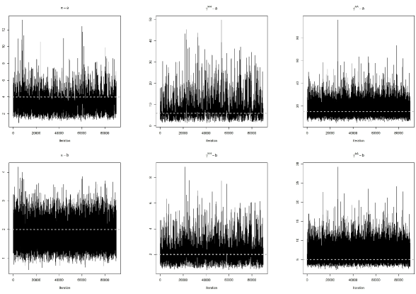
Figure 1: Trace plots for population-level hyper-parameters. Dotted grey lines indicate true values used in simulation of synthetic data. Plots indicate convergence of chains.

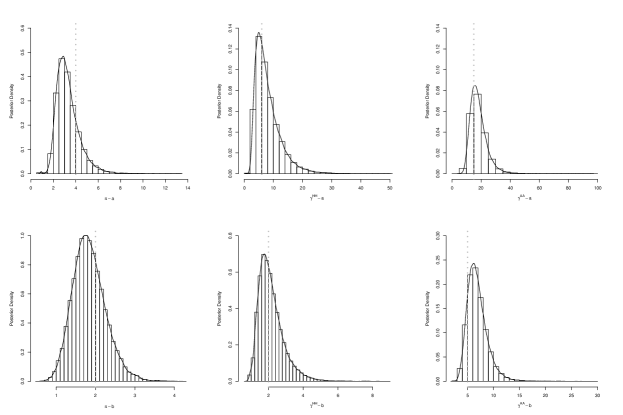
Figure 2: Histogram and density plot of population-level hyper-parameters. Vertical dashed lines indicate true value used to simulate data.

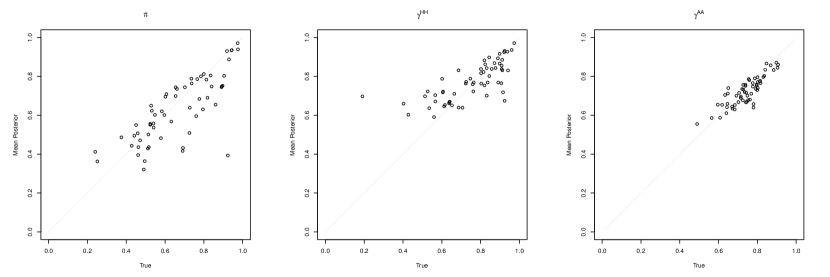
Figure 3: Plot of true values from simulated data vs mean of individual posterior values for probability of Observation, probability of remaining Here and Away.

3.1.2 Asymptotic convergence of $a$ and $b$

The asymptotic convergence of the posterior distribution for each of the hyper-parameters was tested using three simulated data sets with fixed capture histories (length 250) but increasing number of animals (50, 200, 800). For each parameter ($\pi$, $\gamma^{HH}$ and $\gamma^{AA}$), synthetic data was simulated from a $Beta(8,2)$ distribution (i.e. a mean of approximately 0.8). MCMC chains were run for 15000 iterations, with the first 5000 discarded to burn in.

	$\pi$		$\gamma^{HH}$		$\gamma^{AA}$
	$a$	$b$	$a$	$b$	$a$	$b$
TRUTH	8	2	8	2	8	2
50 animals	13.17 ( 6.41 )	2.71 ( 1.00 )	7.34 ( 2.14 )	1.93 ( 0.45 )	10.40 ( 2.60 )	2.33 ( 0.53 )
200 animals	9.47 ( 1.64 )	2.29 ( 0.34 )	7.07 ( 1.17 )	1.77 ( 0.24 )	6.60 ( 0.94 )	1.65 ( 0.19 )
800 animals	7.98 ( 0.88 )	1.97 ( 0.17 )	8.62 ( 0.93 )	2.17 ( 0.17 )	8.77 ( 0.68 )	2.08 ( 0.13 )

Table 1: Means and standard deviations (in brackets) for hyper-parameters from simulated data.

Figure 4 shows density plots of posterior estimates for the six hyper-parameters: decreasing variance is evident with increasing number of individuals. Table 1 indicates posterior standard deviations decreased at the expected rate of approximately $\frac{1}{\sqrt{n}}$ (here $n$ = number of animals).

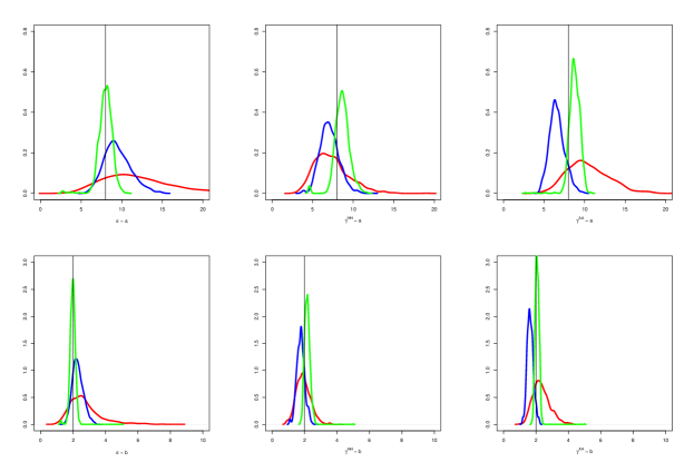
Figure 4: Posterior density plots for each hyper-parameter from simulated data. The red density line is for 50 animals; blue for 200 animals; and green for 800 animals. The vertical black line indicates the true values used to simulate the data.

3.1.3 Convergence of individual mean posterior estimates

Asymptotic convergence for the mean of individual posterior estimates to true individual values (used in simulation) was tested by increasing length of capture history (250, 1000, 4000) for three data sets each with 16 individuals. MCMC chains were run for 15000 iterations, with the first 5000 discarded to burn in. Data were simulated using the following distributions: $\pi\sim Beta(30,3)$, $\gamma^{HH}\sim Beta(30,5)$ and $\gamma^{AA}\sim Beta(30,2)$ (i.e. approximate mean probabilities of 0.91, 0.86, 0.94).

Figure 5 indicates convergence of the mean of individual posterior estimates to true values for each of $\pi$, $\gamma^{HH}$ and $\gamma^{AA}$. Standard deviations decreased with increasing length of capture history, and correlation improved with longer capture histories.

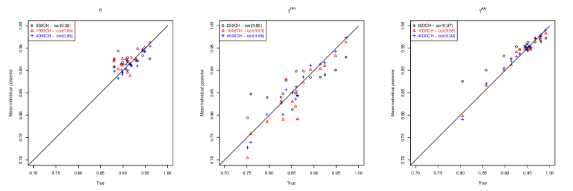
Figure 5: Mean individual posterior values vs true values for $\pi$, $\gamma^{HH}$ and $\gamma^{AA}$ from simulated data. Correlations indicate increasing convergence to true values with increasing length of capture history.

3.2 Results for North Atlantic Humpback whales

One chain was run for 100000 iterations with the first 10000 discarded to burn-in. Figure 6 indicates the trace plots for the first and last 45000 posterior estimates and Figure 7 shows density plots of the mean and standard deviation of logit $\pi$, $\gamma^{HH}$ and $\gamma^{AA}$ (calculated as $mean=\psi(a)-\psi(b)$ and $sd=\sqrt{\psi(a)^{\prime}+\psi(b)^{\prime}}$ where $\psi$ indicates the moment). Both the trace plots and a the mean and standard deviation on the logit scale indicate no visible differences between the first and second half of the chains suggesting that full convergence was reached with 100000 iterations.

Posterior estimates were less varied for $\pi$ compared to $\gamma^{HH}$ and $\gamma^{AA}$. Figure 8 indicates the density for $\pi$, $\gamma^{HH}$ and $\gamma^{AA}$ for all individuals for 90000 iterations. Population-level variability is apparent in $\pi$, but somewhat less so in the two state probabilities. However, Figure 7 indicates that the standard deviation logits are not much smaller for both $\gamma^{HH}$ and $\gamma^{AA}$ compared to $\pi$. Since the transition parameters ($\gamma^{HH}$ and $\gamma^{AA}$) are close to 1, there is less opportunity to see heterogeneity than for $\pi$.

Figure 6: Trace plots of hyper-parameters for $\pi$, $\gamma^{HH}$ and $\gamma^{AA}$ for 90000 posterior estimates for real data. The black trace indicates the first 45000 estimates and the red the final 45000.

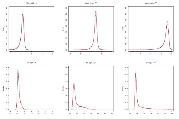
Figure 7: Density plots for the mean and standard deviation of logit$\pi$, $\gamma^{HH}$ and $\gamma^{AA}$ for 90000 posterior estimates for real data. The black line indicates the first 45000 estimates and the red the final 45000.

Figure 8: Density plots from 90000 posterior samples from three independent chains for $\pi$, $\gamma^{HH}$ and $\gamma^{AA}$ for real data.

3.2.1 Fully Bayesian MCMC approach vs Empirical Bayes using ADMB

The same subset of whale (176 individuals seen more than 30 times between 1979 and 2005) was used for the Empirical Bayes model in ADMB. Beta distributed random effects were implemented in ADMB. The model was otherwise the same as described in Ford et al. (2012).

Posterior estimates from the beta-binomial MCMC model were compared with individual posterior results from ADMB. Results appear to be similar, but more variation and slightly lower mean is evident in the Beta-Binomial MCMC results (Figure 9). This difference in variation is likely due to the Beta-Binomial MCMC results incorporating the uncertainty on the hyper-parameters; in comparison ADMB results are conditioned on point estimates of the hyper-parameters.

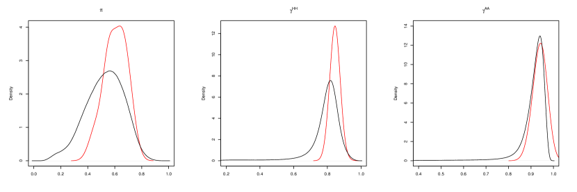
Figure 9: Comparison of posterior samples for $\pi$, $\gamma^{HH}$ and $\gamma^{AA}$ for Beta-Binomial MCMC sampler and individual posterior estimates from ADMB.

4 Discussion

We have developed a hierarchical Bayesian hidden Markov model where individual parameters are updated using Gibbs sampling, the population-level hyper-parameters and fixed-effects using an Independent Metropolis-Hastings sampler. Results from simulation tests indicate asymptotic convergence for both individual and population-level parameters: the posterior standard deviations for the population-level parameters decreased with increasing number of individuals, and correlation for mean posterior individual estimates to true values improved with increasing length of capture history.

The Beta-binomial model we presented in this paper is an efficient MCMC routine for incorporating individual heterogeneity into mark-recapture models. The Independent sampler in particular provides an efficient method to update parameter values when a Gibbs sampler cannot be implemented. The Independent sampler is almost efficient as the Gibbs sampler and avoids the difficulties which can arise with standard Metropolis-Hastings routines, namely the need to tune random walk sizes.

Output from ADMB was used to facilitate sampling from a multivariate t-distribution in order to update the fixed parameters in the model. This resulted in an automatic and computationally efficient method to update these complex model parameters, avoiding the need to tweak, for example, random walk step sizes. This method can also be used to incorporate covariates into the model, providing another extension to the already flexible model. We note here that we used Laplace Approximation results from ADMB in order to inform the fully Bayesian approach using the Beta-binomial MCMC sampler. This provided an efficient and effective method to update the MCMC sampler.

In Empirical Bayes methods (using Laplace Approximation), the hyper-parameter is estimated from the data and set to it’s maximum likelihood estimate. In comparison, in a fully Bayes approach the hyper-parameter is endowed with a prior distribution. Thus the MCMC approach automatically incorporates uncertainty into the hyper-parameters. We presented results from a beta-binomial model implemented purely in ADMB. The ADMB software does include an MCMC option, however our experience was that it ran extremely slowly before eventually crashing due to memory constraints. Thus we were unable to obtain full MCMC results from ADMB (using version 11). If this situation is rectified in future releases of the software a full Bayesian version of the approach may avoid the need to resort to MCMC. While our experience was that MCMC was quicker and worked, it did require significant use of ADMB estimation in order to inform the MCMC. This demonstrates that in real situations, hybrid approaches can be particularly useful in getting complex multi-state models to perform reliably.

The approach we present in this paper, presents a tractable Bayesian method to estimate multi-state mark-recapture models which incorporate individual heterogeneity on process and observation model parameters. As MCMC samplers go it is computationally efficient and therefore allows for thorough model checking via simulation. Our application to data from humpback whales indicated heterogeneity in both site fidelity and sighting probability. This indicates heterogeneity in propensity to use the marine sanctuary both on a population and individual-level. The role of individuals in mediating population processes has been a key question in ecology but it is often one that is side-stepped in management and conservation applications. In this paper we have demonstrated an analytical tool which we hope will begin to fill this gap.

References

- Arnason (1972) Arnason, A. N. 1972. Parameter estimates from mark-recapture experiments on two populations subject to migration and death. Researches in Population Ecology, 13(2):97–113.
- Arnason (1973) Arnason, A. N. 1973. The estimation of population size, migration rates, and survival in a stratified population. Researches on Population Ecology, 15(1):1–8.
- Barry et al. (2003) Barry, S. C., Brooks, S. P., Catchpole, E., and Morgan, B. 2003. The analysis of ring-recovery data using random effects. Biometrics, 59(1):54–65.
- Burnham and Overton (1978) Burnham, K. P. and Overton, W. S. 1978. Estimation of size of a closed population when capture probabilities vary among animals. Biometrika, 65(3):625–633.
- Clapham and Mead (1999) Clapham, P. and Mead, J. 1999. Megaptera novaeangliae. Mammalian Species, 604:1–9.
- Conn and Cooch (2009) Conn, P. B. and Cooch, E. G. 2009. Multistate capture-recapture analysis under imperfect state observation: an application to disease models. Journal of Applied Ecology, 46(2):486–492.
- Crespin et al. (2008) Crespin, L., Choquet, R., Lima, M., Merritt, J., and Pradel, R. 2008. Is heterogeneity of catchability in capture-recapture studies a mere sampling artifact or a biologically relevant feature of the population? Population Ecology, 50(3):247–256.
- Cubaynes et al. (2012) Cubaynes, S., Lavergne, C., Marboutin, E., and Gimenez, O. 2012. Assessing individual heterogeneity using model selection criteria: how many mixture components in capture-recapture models? Methods in Ecology and Evolution, 3:564–573.
- D’Agrosa et al. (2000) D’Agrosa, C., Lennert-Cody, C., and Vidal, O. 2000. Vaquita bycatch in mexico’s artisanal gillnet fisheries: Driving a small population to extinction. Conservation Biology, 14(4):1110–1119.
- Ford et al. (2012) Ford, J., Bravington, M., and Robbins, J. 2012. Incorporating individual variability into mark-recapture models. Methods in Ecology and Evolution, 3:1047–1054.
- Fournier et al. (2012) Fournier, D. A., Skaug, H., Ancheta, J., Ianelli, J., Magnusson, A., Maunder, M., Nielsen, A., and Sibert, J. 2012. AD model builder: using automatic differentiation for statistical inference of highly parameterized complex nonlinear models. Optimization Methods & Software, 27:2:233–249.
- Franklin et al. (2000) Franklin, A., Anderson, D., Gutierrez, J., and Burnham, K. 2000. Climate, habitat quality, and fitness in northern spotted owl populations in northwestern california. Ecological Monographs, 70(4):539–590.
- Gilks et al. (1996) Gilks, W., Richardson, S., and Spiegelhalter, D. 1996. Markov Chain Monte Carlo in Practice. Chapman and Hall /CRC.
- Gimenez and Choquet (2010) Gimenez, O. and Choquet, R. 2010. Individual heterogeneity in studies on marked animals using numerical integration: capture-recapture mixed models. Ecology, 91(4):951–957.
- Gimenez et al. (2012) Gimenez, O., Lebreton, J. D., Gaillard, J.-M., Choquet, R., and Pradel, R. 2012. Estimating demographic parameters using hidden process dynamic models. Theoretical Population Biology, 82(4):307–16.
- Grimm and Uchmanski (2002) Grimm, V. and Uchmanski, J. 2002. Individual variability and population regulation: a model of the significance of within-generation density dependence. Oecologia, 131:196–202.
- Hammond (1986) Hammond, P. S. 1986. Estimating the size of naturally marked whale populations using capture-recapture techniques. Reports of the International Whaling Commission., (Special Issue) 8:253–282.
- Hammond (1990) Hammond, P. S. 1990. Heterogeneity in the gulf of maine? estimating humpback whale population size when capture probabilities are not equal. Reports of the International Whaling Commission, (Special Issue) 12:135–139.
- Hoyt (2011) Hoyt, E. 2011. Marine Protected Areas for Whales, Dolphins and Porpoises: A World Handbook for Cetacean Habitat Conservation and Planning. Earthscan, London and Washington.
- Huggins and Yip (2001) Huggins, R. M. and Yip, P. S. F. 2001. Note on nonparametric inference for capture-recapture experiments with heterogeneous capture probabilities. Statistica Sinica, 11(3):843–853.
- Johnson et al. (2005) Johnson, A., Salvador, G., Kenney, J., Robbins, J., Kraus, S., Landry, S., and Clapham, P. 2005. Fishing gear involved in entanglements of right and humpback whales. Marine Mammal Science, 21(4):635–645.
- Knowlton and Kraus (2001) Knowlton, A. and Kraus, S. 2001. Mortality and serious injury of northern right whales (Eubalaena glacialis) in the western north atlantic ocean. Journal of Cetacean Research and Management, (Special Issue) 2:193–208.
- Laist et al. (2001) Laist, D., Knowlton, A., Mead, J., Collet, A., and Podesta, M. 2001. Collisions between ships and whales. Marine Mammal Science, 17:35–75.
- Lebreton et al. (1992) Lebreton, J. D., Burnham, K. P., Clobert, J., and Anderson, D. 1992. Modeling survival and testing biological hypotheses using marked animals, a unified approach with case studies. Ecological Monographs, 62:67–118.
- Lebreton et al. (2009) Lebreton, J. D., Nichols, J. D., Barker, R., Pradel, R., and Spendelow, J. 2009. Modeling individual animal histories with multistate capture-recapture models. In Hal Caswell, editor: Advances in Ecological Research, 41:87–173.
- Lebreton and Pradel (2002) Lebreton, J. D. and Pradel, R. 2002. Multistate recapture models: modelling incomplete individual histories. Journal of Applied Statistics, 29(1-4):353–369.
- Maunder et al. (2008) Maunder, M., Skaug, H., Fournier, D., and Hoyle, S. 2008. Comparison of estimators for mark-recapture models: random effects, hierarchical bayes, and ad model builder. In In: Modeling Demographic Processes in Marked Populations. Eds. Thomson, D.L., Cooch, E.G., and Conroy, M.J. Environmental and Ecological Statistics, volume 3, pages 917–948.
- Norris and Pollock (1996) Norris, J. and Pollock, K. 1996. Nonparametric mle under two closed capture-recapture models with heterogeneity. Biometrics, 52:639–649.
- Patterson et al. (2008) Patterson, T. A., Thomas, L., Wilcox, C., Ovaskainen, O., and Matthiopoulos, J. 2008. State-space models of individual animal movement. Trends in Ecology & Evolution, 23(2):87–94.
- Pledger (2000) Pledger, S. 2000. Unified maximum likelihood estimates for closed capture-recapture models using mixtures. Biometrics, 56:434–442.
- Pledger et al. (2010) Pledger, S., Pollock, K., and Norris, J. 2010. Open capture-recapture models with heterogeneity: Ii. jolly-seber model. Biometrics, 66(3):883–890.
- Pradel (2005) Pradel, R. 2005. Multievent: An extension of multistate capture-recapture models to uncertain states. Biometrics, 61(2):442–447.
- Read et al. (2006) Read, A., Drinker, P., and Northridge, S. 2006. Bycatch of marine mammals in u.s. and global fisheries. Conservation Biology, 20:163–169.
- Royle and Dorazio (2008) Royle, J. A. and Dorazio, R. M. 2008. Hierarchical modeling and inference in ecology: the analysis of data from populations, metapopulations and communities, volume i-xviii. London, Academic Press Elsevier.
- Scott (2002) Scott, S. 2002. Bayesian methods for hidden markov models, recursive computing in the 21st century. Journal of the American Statistical Association, 97:337–351.
- Vieilledent et al. (2010) Vieilledent, G., Courbaud, B., Kunstler, G., Dhote, J.-F., and Clark, J. 2010. Individual variability in tree allometry determines light resource allocation in forest ecosystems: a hierarchical bayesian approach. Oecologia, 163:759–773.
- Wilgart (2007) Wilgart, L. 2007. The impacts of anthropogenic ocean noise on cetaceans and implications for management. Can. J. Zool., 85:1091–1116.
- Zucchini and MacDonald (2009) Zucchini, W. and MacDonald, I. 2009. Hidden Markov Models for Time Series An Introduction Using R. Chapman and Hall / CRC.
- Zucchini et al. (2008) Zucchini, W., Raubenheimer, D., and MacDonald, I. 2008. Modeling time series of animal behavior by means of a latent-state model with feedback. Biometrics, 64(3):807–815.