Majorization entropic uncertainty relations for quantum operations

Abstract

Majorization uncertainty relations are derived for arbitrary quantum operations acting on a finite-dimensional space. The basic idea is to consider submatrices of block matrices comprised of the corresponding Kraus operators. This is an extension of the previous formulation, which deals with submatrices of a unitary matrix relating orthogonal bases in which measurements are performed. Two classes of majorization relations are considered: one related to tensor product of probability vectors and another one related to their direct sum. We explicitly discuss an example of a pair of one-qubit operations, each of them represented by two Kraus operators. In the particular case of quantum maps describing orthogonal measurements the presented formulation reduces to earlier results derived for measurements in orthogonal bases. The presented approach allows us also to bound the entropy characterizing results of a single generalized measurement.

I Introduction

The Heisenberg uncertainty relation wh27 is one of the fundamental limitations in description of the quantum world. It is commonly emphasized that one is unable to assign simultaneously precise values to non-commuting observables. Despite a vast literature concerning the uncertainty relations, there is an on going debate over their scope and validity lahti ; hall99 . The traditional formulation of Robertson robert gives a lower bound on the product of the standard deviations of two observables. This state-dependent bound is proportional to the modulus of the expectation value of the commutator in the measured state. Dependence on the pre-measurement state results in the fact that Robertson’s bound may vanish, even if the commutator itself is non-zero. For instance, a trivial bound is obtained for any eigenstate of any of the two observables maass . Relations with a lower bound on product of the standard deviations are useful for a small class of quantum observables zimba00 .

There are several other approaches to measure the amount of uncertainty in quantum measurements. Entropic uncertainty relations are currently the subject of a considerable scientific interest ww10 ; brud11 ; cbtw15 . For the case of canonically conjugate variables, this approach was initiated by Hirschman hirs and later developed in beck ; birula1 . Advantages of entropic uncertainty relations for finite-dimensional systems were emphasized in deutsch ; kraus87 . The famous result of Maassen and Uffink maass is based on the Riesz theorem and inspires many later formulations. Entropic uncertainty relations were derived for several special measurements such as mutually unbiased bases ivan92 ; sanchez93 ; molm09a . This question was further examined with use of both the generalized entropies of Rényi and Tsallis rastmub . Another viewpoint on the Maassen–Uffink bound is connected with the role of a quantum memory BCCRR10 . Improved entropic uncertainty relations in the presence of quantum correlations were obtained in coles14 .

As was emphasized in oppwn10 , entropic bounds cannot distinguish the uncertainty inherent in obtaining a particular combination of the outcomes. Studies of the fine-grained uncertainty relations were initiated in oppwn10 and further developed in renf13 ; rastqip15 ; Rud15 . Majorization relations offer an alternative way to express the uncertainty principle in terms of probabilities per se prtv11 . At the same time, majorization relations directly lead to desired inequalities in terms of the Shannon entropy or other generalized entropies. First majorization entropic uncertainty relations were based on tensor product of probability vectors prz13 ; fgg13 . Even stronger bounds obtained in rpz14 are based on majorization relations applied to direct-sum of probability vectors.

In this work we extend the techniques applied in prz13 ; rpz14 for orthogonal projective measurements for any trace-preserving quantum operations in finite dimensions. This issue was already discussed in fgg13 , but our present results go much further and lead to explicit bounds easy to apply in the general case. The case of POVM measurements is included into discussion, as quantum measurements can be described in terms of Kraus operators. In our approach we use the majorization techniques for vectors depending on norms of submatrices. In the case of orthogonal measurements, the authors of prz13 ; rpz14 used submatrices of a unitary matrix, relating both bases. In this work, concerning the general case of arbitrary quantum operations, we consider submatrices of block matrices formed by concatenation of Kraus operators, which represent the quantum operation. Majorization uncertainty relations obtained in this work are compared with generalizations of the Maassen–Uffink bounds for quantum operations KP902 ; rast104 .

The paper is organized as follows. In Sect. II, we review required notions and preliminary facts of matrix analysis. Previous results on majorization uncertainty relations are briefly discussed in Sect. III. The majorization uncertainty relations for quantum operations are obtained in Sect. IV. In Sect. V we consider an example of two quantum operations acting on a single qubit and represented by two Kraus operators each. Majorization bounds derived here are compared with uncertainty relations of the Maassen–Uffink type. In Sect. VI, we show that in the case of two orthogonal measurements the proposed formulation reduces to the former one. The paper is concluded in Sect. VII with a brief summary of results obtained. In A, we apply of the majorization approach to the case of a single quantum operation.

II Preliminaries

In this section, preliminary facts are briefly outlined. For any two integers $m,n\geq 1$ the symbol $\mathbb{M}_{m\times{n}}(\mathbb{C})$ denotes the space of all $m\times{n}$ complex matrices hiai2014 . If $m=n$, we will usually write $\mathbb{M}_{n}(\mathbb{C})$. Each matrix ${\mathsf{X}}\in\mathbb{M}_{m\times{n}}(\mathbb{C})$ can be represented in terms of the singular value decomposition hj1990 ,

$${\mathsf{X}}={\mathsf{U}}{\mathsf{\Sigma}}{\mathsf{V}}^{\dagger}\ ,$$ (1)

where ${\mathsf{U}}\in\mathbb{M}_{m}(\mathbb{C})$ and ${\mathsf{V}}\in\mathbb{M}_{n}(\mathbb{C})$ are unitary. The matrix ${\mathsf{\Sigma}}=[[\sigma_{ij}]]\in\mathbb{M}_{m\times{n}}(\mathbb{C})$ has $\sigma_{ij}=0$ for all $i\neq{j}$. If the given matrix ${\mathsf{X}}$ has rank $k$, then we can write ${\mathsf{\Sigma}}$ so that

$$\sigma_{11}\geq\cdots\geq\sigma_{kk}>\sigma_{k+1,k+1}=\cdots=\sigma_{rr}=0\ ,$$ (2)

where $r=\min\{m,n\}$. The diagonal entries $\{\sigma_{jj}\}=\{\sigma_{j}({\mathsf{X}})\}$ of ${\mathsf{\Sigma}}$ are known as the singular values of ${\mathsf{X}}$. The non-zero $\sigma_{jj}$’s are the squared roots of positive eigenvalues of both ${\mathsf{X}}{\mathsf{X}}^{\dagger}$ and ${\mathsf{X}}^{\dagger}{\mathsf{X}}$. A coordinate-independent formulation of the above facts can be found in watrous1 .

We will use the notion of the spectral norm of a matrix, which can be written in terms of the singular values,

$$\|{\mathsf{X}}\|_{\infty}=\max\bigl{\{}\sigma_{j}({\mathsf{X}}):{\>}1\leq{j}\leq{r}\bigr{\}}\ .$$ (3)

It is sometimes referred to as the operator norm. Other norms are widely used in quantum information theory watrous1 for quantifying various properties of a matrix. Many of them are also defined in terms of singular values. For instance, the Schatten norms form an important family of unitarily invariant norms. A norm $||\centerdot||$ is said to be unitarily invariant if

$$||{\mathsf{U}}{\mathsf{X}}{\mathsf{V}}||=||{\mathsf{X}}||$$ (4)

for all ${\mathsf{X}}\in\mathbb{M}_{m\times{n}}(\mathbb{C})$ and for all unitary matrices ${\mathsf{U}}\in\mathbb{M}_{m}(\mathbb{C})$, ${\mathsf{V}}\in\mathbb{M}_{n}(\mathbb{C})$ hj1990 . We will also exploit the following two facts. Let ${\mathsf{X}}$ and ${\mathsf{Y}}$ be two rectangular matrices of the same size. Then the products ${\mathsf{X}}{\mathsf{Y}}^{\dagger}$ and ${\mathsf{Y}}^{\dagger}{\mathsf{X}}$ have the same non-zero eigenvalues. If ${\mathsf{X}}$ is a submatrix of ${\mathsf{Y}}$, then $\|{\mathsf{X}}\|_{\infty}\leq\|{\mathsf{Y}}\|_{\infty}$.

The space of linear operators on finite-dimensional Hilbert space $\mathcal{H}$ will be denoted as ${\mathcal{L}}(\mathcal{H})$. By ${\mathcal{L}}_{s.a.}(\mathcal{H})$ and ${\mathcal{L}}_{+}(\mathcal{H})$ we mean the real space of Hermitian operators and the set of positive operators, respectively. Let square matrices ${\mathsf{X}}$ and ${\mathsf{Y}}$ represent elements of ${\mathcal{L}}(\mathcal{H})$. Their Hilbert–Schmidt product is defined as watrous1

$$\langle{\mathsf{X}}{\,},{\mathsf{Y}}\rangle_{\mathrm{hs}}:={\mathrm{Tr}}({\mathsf{X}}^{\dagger}{\mathsf{Y}})\ .$$ (5)

This inner product induces the Hilbert–Schmidt norm of matrices. If the reference basis is fixed, we can avoid distinguishing between elements of ${\mathcal{L}}(\mathcal{H})$ and these matrices which represent them. We shall prove another statement concerning the spectral norm.

Lemma 1

Let ${\mathsf{X}}$ be a rectangular matrix, and let ${\mathsf{Y}}$ be obtained from ${\mathsf{X}}$ by adding rows of zeros and columns of zeros. Then these matrices have the same spectral norm, i.e., $\|{\mathsf{X}}\|_{\infty}=\|{\mathsf{Y}}\|_{\infty}$.

Proof. Without loss of generality, we assume that zero rows are placed below and zero columns are added right. This is merely rearranging of vectors of the standard basis. So, we can write

$${\mathsf{Y}}=\begin{pmatrix}{\mathsf{X}}&\mathbf{0}\\ \mathbf{0}&\mathbf{0}\end{pmatrix},$$

where $\mathbf{0}$’s are zero submatrices. Due to (1), we further obtain

$${\mathrm{diag}}({\mathsf{U}},\openone)\,{\mathsf{Y}}\,{\mathrm{diag}}({\mathsf{V}}^{\dagger},\openone)=\begin{pmatrix}{\mathsf{\Sigma}}&\mathbf{0}\\ \mathbf{0}&\mathbf{0}\end{pmatrix}.$$ (6)

By $\openone$, we mean the identity matrices of the corresponding size. Formula (6) shows that non-zero singular values of the matrices ${\mathsf{X}}$ and ${\mathsf{Y}}$ are the same. $\blacksquare$

To approach majorization uncertainty relations, the authors of prz13 ; rpz14 inspected norms of submatrices of a certain unitary matrix. To the given two orthonormal bases $\{|e_{i}\rangle\}$ and $\{|f_{j}\rangle\}$, with $i,j=1,\ldots,d$, we assign the unitary matrix ${\mathsf{W}}$ of size $d$ with entries $w_{ij}=\langle{e}_{i}|f_{j}\rangle$. By $\mathcal{SUB}({\mathsf{W}},k)$, we mean the set of all its submatrices of class $k$ defined by

$$\mathcal{SUB}({\mathsf{W}},k):=\bigl{\{}{\mathsf{M}}\in\mathbb{M}_{r\times{r}^{\prime}}(\mathbb{C}):{\>}r+r^{\prime}=k+1,{\>}{\mathsf{M}}{\text{ is a submatrix of }}{\mathsf{W}}\bigr{\}}\,.$$ (7)

The positive integer $k$ runs all the values, for which the following condition for sum of integer dimensions holds, $r+r^{\prime}=k+1$. The majorization relations of prz13 ; rpz14 are expressed in terms of quantities

$$s_{k}:=\max\bigl{\{}\|{\mathsf{M}}\|_{\infty}:{\>}{\mathsf{M}}\in\mathcal{SUB}({\mathsf{W}},k)\bigr{\}}\,.$$ (8)

This definition can be extended to an arbitrary matrix and, furthermore, to a block matrix. Let ${\mathsf{X}}$ be a $M\times{N}$ matrix of blocks ${\mathsf{X}}_{ij}$, each of size $d$, namely

$${\mathsf{X}}=\begin{pmatrix}{\mathsf{X}}_{11}&\cdots&{\mathsf{X}}_{1N}\\ \cdots&\cdots&\cdots\\ {\mathsf{X}}_{M1}&\cdots&{\mathsf{X}}_{MN}\end{pmatrix}.$$ (9)

Calculations with block matrices are similar to these with ordinary matrices hiai2014 . We should only remember that their entries do not commute. Block submatrices of (9) are defined quite similarly to submatrices of ordinary matrices. That is, one fixes a subset of rows and a subset of columns in (9). Keeping the blocks on the points of intersection will result in a submatrix composed of some $d\times{d}$ blocks of ${\mathsf{X}}$. This definition should not lead to a confusion since the size of blocks is prescribed initially. We will now extend definitions (7) and (8). Let us define the set

$$\mathcal{BSUB}({\mathsf{X}},k):=\Bigl{\{}{\mathsf{Z}}\in\mathbb{M}_{rd\times{r}^{\prime}d}(\mathbb{C}):{\>}r+r^{\prime}=k+1,{\>}{\mathsf{Z}}{\text{ is a submatrix of $d\times{d}$-blocks of ${\mathsf{X}}$}}\Bigr{\}}\,.$$ (10)

Again, the positive integer $k$ runs all the values with respect to $r+r^{\prime}=k+1$. For $M\times{N}$ block matrix (9), we have $1\leq{k}\leq{M}+N-1$. Similarly to (8), we further introduce a sequence with positive elements

$$c_{k}:=\max\bigl{\{}\|{\mathsf{Z}}\|_{\infty}:{\>}{\mathsf{Z}}\in\mathcal{BSUB}({\mathsf{X}},k)\bigr{\}}\,.$$ (11)

The aim of the present work is to extend the techniques applied in prz13 ; rpz14 for orthogonal measurements for trace-preserving completely positive maps, also called quantum operations or stochastic maps. Let us recall some basic notions of the field. We will consider a linear map $\Phi:\,{\mathcal{L}}(\mathcal{H})\rightarrow{\mathcal{L}}(\mathcal{H}^{\prime})$ that takes elements of ${\mathcal{L}}(\mathcal{H})$ to elements of ${\mathcal{L}}(\mathcal{H}^{\prime})$. This map is called positive, when elements of ${\mathcal{L}}_{+}(\mathcal{H})$ are mapped to elements of ${\mathcal{L}}_{+}(\mathcal{H}^{\prime})$ bhatia07 . To describe physical processes, linear maps have to be completely positive bengtsson ; nielsen . Let ${\mathrm{id}}^{\prime\prime}$ be the identity map on ${\mathcal{L}}(\mathcal{H}^{\prime\prime})$, where the space $\mathcal{H}^{\prime\prime}$ is assigned to a reference system. Complete positivity implies that the map $\Phi\otimes{\mathrm{id}}^{\prime\prime}$ is positive for any dimension of the auxiliary space $\mathcal{H}^{\prime\prime}$. A completely positive map $\Phi$ can be written by an operator-sum representation. For the input density matrix $\boldsymbol{\rho}\in{\mathcal{L}}_{+}(\mathcal{H})$, the output one is then written as

$$\Phi(\boldsymbol{\rho})=\sum\nolimits_{i}{\mathsf{A}}_{i}\boldsymbol{\rho}\,{\mathsf{A}}_{i}^{\dagger}\ .$$ (12)

Here, the Kraus operators ${\mathsf{A}}_{i}$ map the input space $\mathcal{H}$ to the output space $\mathcal{H}^{\prime}$. They are described by matrices with ${\mathrm{dim}}(\mathcal{H}^{\prime})$ rows and ${\mathrm{dim}}(\mathcal{H})$ columns. Representations of the form (12) are not unique watrous1 . Each concrete set $\{{\mathsf{A}}_{i}\}$ resulting in (12) will be referred to as “unraveling” of the map $\Phi$. This terminology is due to Carmichael carm who introduced this notion to represent master equations. If a physical process is closed and the probability is conserved, the map preserves the trace:

$${\mathrm{Tr}}\bigl{(}\Phi(\boldsymbol{\rho})\bigr{)}={\mathrm{Tr}}(\boldsymbol{\rho})\ .$$ (13)

This relation satisfied for all $\boldsymbol{\rho}$ is equivalent to the following constraint for the set of the Kraus operators:

$$\sum\nolimits_{i}{\mathsf{A}}_{i}^{\dagger}{\mathsf{A}}_{i}=\openone\ .$$ (14)

Here $\openone$ denotes the identity operator on the input space $\mathcal{H}$.

A general quantum measurement can be described by a collection of measurement operators nielsen . These measurement operators obey the relation (14), so we can treat them as Kraus operators. If the pre-measurement state is described by a density matrix $\boldsymbol{\rho}\in{\mathcal{L}}_{+}(\mathcal{H})$, normalized as ${\mathrm{Tr}}(\boldsymbol{\rho})=1$, then the probability of $i$-th outcome is written as ${\mathrm{Tr}}\bigl{(}{\mathsf{A}}_{i}^{\dagger}{\mathsf{A}}_{i}\boldsymbol{\rho}\bigr{)}$. When we are interested only in the probabilities of the respective outcomes, we may restrict an attention to positive semidefinite operators ${\mathsf{E}}_{i}={\mathsf{A}}_{i}^{\dagger}{\mathsf{A}}_{i}$. The set $\{{\mathsf{E}}_{i}\}$ gives a non-orthogonal resolution of the identity often called positive operator-valued measure (POVM). Thus, the POVM formalism to deal with quantum measurements is naturally involved into our approach. We only note that measurement operators give a more refined description of the measurement process.

For any quantum operation $\Phi$ one has a certain freedom in the operator-sum representation. Suppose that the set $\{\widetilde{\mathsf{A}}_{i}\}$ is another unraveling of the quantum operation (12). Then the Kraus operators are related as

$$\widetilde{{\mathsf{A}}}_{i}=\sum\nolimits_{j}\gamma_{ij}{\,}{\mathsf{A}}_{j}\ ,$$ (15)

where the matrix ${\mathsf{\Gamma}}=[[\gamma_{ij}]]$ is unitary nielsen . Here, we assume that the sets $\mathcal{A}=\{{\mathsf{A}}_{i}\}$ and $\widetilde{\mathcal{A}}=\{\widetilde{{\mathsf{A}}}_{i}\}$ have the same cardinality by adding zero operators, if needed. A size of the matrix ${\mathsf{\Gamma}}$ corresponds to this cardinality.

Finally, we recall some notions of majorization. Let $x=(x_{1},\ldots,x_{N})$ and $y=(y_{1},\ldots,y_{N})$ be vectors in $\mathbb{R}^{N}$. The majorization ${x}\prec{y}$ implies that hiai2014

$$\sum\nolimits_{i=1}^{k}x_{i}^{\downarrow}\leq\sum\nolimits_{i=1}^{k}y_{i}^{\downarrow}\qquad(1\leq{k}\leq{N})\ ,$$ (16)

and equality is required for $k=N$. Here the arrows down imply that the components should be put in the decreasing order. As was discussed in prtv11 ; prz13 ; fgg13 ; rpz14 , the uncertainty principle may sometimes be expressed by a majorization relation.

III Majorization uncertainty relations for two von Neumann measurements

In this section, we briefly discuss a general formulation of majorization uncertainty relations for two von Neumann measurements. Definitions of the used entropic measures are recalled as well. To each von Neumann measurement, we can assign some orthogonal resolution of the identity. We first suppose that measured observables are non-degenerate, whence the orthogonal projectors are all of rank-one. It will be convenient to write the dimensionality explicitly. Thus, we deal with two orthonormal bases in $d$-dimensional Hilbert space $\mathcal{H}_{d}$. In any prescribed basis, vectors $|\psi\rangle\in\mathcal{H}_{d}$ are represented as elements of $\mathbb{M}_{d\times 1}(\mathbb{C})$.

Let us consider two orthonormal bases denoted by $\{|e_{i}\rangle\}$ and $\{|f_{j}\rangle\}$ with $i,j=1,\ldots,d$. If the pre-measurement state is described by the normalized density matrix $\boldsymbol{\rho}\in{\mathcal{L}}_{+}(\mathcal{H}_{d})$, then elements of the generated probabilistic vectors $p$ and $q$ are expressed as

$$p_{i} =\langle{e}_{i}|\boldsymbol{\rho}|e_{i}\rangle\ ,$$ (17)

$$q_{j} =\langle{f}_{j}|\boldsymbol{\rho}|f_{j}\rangle\ .$$ (18)

There are several ways to formulate uncertainty relations. In this approach, entropic functions are used to quantify an amount of uncertainty associated with a generated probability distribution. We will use both the Rényi and the Tsallis entropies.

For $0<\alpha\neq 1$, the Rényi $\alpha$-entropy is defined as renyi61

$$H_{\alpha}(p):=\frac{1}{1-\alpha}{\>}\ln\!\left(\sum\nolimits_{i=1}^{d}p_{i}^{\alpha}\right)\,.$$ (19)

This entropy is a non-increasing function of the Rényi parameter $\alpha$ renyi61 . Quantum information measures of the Rényi type are examined in mdsft13 ; berta15 . The Tsallis $\alpha$-entropy of degree $0<\alpha\neq 1$ is defined by tsallis

$$T_{\alpha}(p):=\frac{1}{1-\alpha}{\>}\left(\sum\nolimits_{i=1}^{d}p_{i}^{\alpha}-1\right)\,.$$ (20)

Quantum applications of Tsallis entropic functions are considered in sudha14 ; rast15ap ; rast16a . In the limit $\alpha\to 1$, both entropies (19) and (20) lead to the Shannon entropy

$$H_{1}(p)=-\sum\nolimits_{i=1}^{d}p_{i}\ln{p}_{i}\ .$$ (21)

Note that for $\alpha\to 1$ the Tsallis entropy tends to the Shannon entropy if the latter quantity is defined via natural logarithm as in (21). If required, one can rescale the above formulas in order to change the base of the logarithm. In the following, we will use the fact that entropies (19) and (20) are both Schur concave. Many properties of entropies (19) and (20) and their applications are discussed in the book bengtsson .

We now recall some details of the majorization approach in finite dimensions. Applications of this approach to the case of position and momentum are discussed in prtv11 . Suppose $p$ and $q$ denote two probability vectors generated by two quantum measurements performed on two copies of the same quantum state. The key idea of this approach is to majorize some binary combination of $p$ and $q$ by a third vector with bounding elements. Majorization relations of the tensor-product type, first considered in fgg13 ; prz13 , are obtained by finding a probability vector $\omega^{\prime}$ such that the following majorization relation holds,

$$p\otimes{q}\prec\omega^{\prime}\ .$$ (22)

In the present paper, we also deal with majorization relations of the direct-sum type originally introduced in rpz14 . This approach, usually producing stronger bounds, is based on the relation

$$p\oplus{q}\prec\{1\}\oplus\omega\ ,$$ (23)

where a suitable probability vector $\omega$ has to be found.

For any pair of observables, the vectors $\omega$ and $\omega^{\prime}$ can be obtained within the following procedure. Let $d$-dimensional probabilistic vectors $p$ and $q$ be described according to (17) and (18), respectively. It was shown in rpz14 that these probabilistic vectors obey (23) with

$$\omega=(s_{1},s_{2}-s_{1},\ldots,s_{d}-s_{d-1})\ .$$ (24)

The sequence of positive elements $s_{k}$ is determined by (7) and (8) with the unitary matrix ${\mathsf{W}}=\bigl{[}\bigl{[}\langle{e}_{i}|f_{j}\rangle\bigr{]}\bigr{]}$. Strictly speaking, the integer subscript $k$ in (8) ranges from $1$ up to $d^{2}-1$. It is easy to see, however, that $s_{d}=1$ in the case of two orthonormal bases. Next numbers of the sequence $\{s_{k}\}$ will be $1$ as well. So, we have discarded several zeros from the right-hand side of (24). An earlier result derived in prz13 can be written as (22), where

$$\omega^{\prime}=(t_{1},t_{2}-t_{1},\ldots,t_{d}-t_{d-1})\ ,\qquad t_{k}=\frac{(1+s_{k})^{2}}{4}\ .$$ (25)

In principle, majorization relations (22) and (23) already impose some restrictions on the probabilistic vectors $p$ and $q$. Moreover, they can be easily converted into entropic uncertainty relations. As the Rényi entropy is Schur concave, the majorization relation (22) leads to the following bounds for Rényi entropy with $\alpha>0$ fgg13 ; prz13 ,

$$H_{\alpha}(p)+H_{\alpha}(q)\geq{H}_{\alpha}(\omega^{\prime})\ .$$ (26)

The authors of fgg13 also used majorization relations of the tensor-product type. They formulate an optimization problem for finding a majorizing vector in (22). This problem can be easily extended to the case of several POVM measurements. However, since no general, effective algorithm for solving the optimization problem is available, in this work we extend other techniques applied for orthogonal measurements in prz13 .

As was shown in rpz14 , majorization relation (23) allows one to improve entropic bounds. For $0<\alpha\leq 1$, we have

$$H_{\alpha}(p)+H_{\alpha}(q)\geq{H}_{\alpha}(\omega)\ .$$ (27)

This bound is stronger, since $\omega\prec\omega^{\prime}$ and, herewith, $H_{\alpha}(\omega)\geq{H}_{\alpha}(\omega^{\prime})$ rpz14 . For $\alpha>1$ relation (27) does not hold. However, in the case $\alpha>1$ the sum of two Rényi entropies satisfies another inequality rpz14

$$H_{\alpha}(p)+H_{\alpha}(q)\geq\frac{2}{1-\alpha}{\>}\ln\!\left(\frac{1}{2}+\frac{1}{2}\,\sum\nolimits_{i=1}^{d}\omega_{i}^{\alpha}\right)\,.$$ (28)

It turned out that the sum of two Tsallis $\alpha$-entropies is bounded from below similarly to (27). For any $\alpha>0$ we have

$$T_{\alpha}(p)+T_{\alpha}(q)\geq{T}_{\alpha}(\omega)\ .$$ (29)

Extensions of the above majorization relations to several orthonormal bases are discussed in prz13 ; rpz14 . We aim to generalize majorization relations in another direction connected with quantum operations.

IV Majorization uncertainty relations for two quantum operations

In this section, we formulate majorization uncertainty relations for a pair of trace-preserving quantum operations. For simplicity, we focus on the case of the same dimensionality of the input and output states. Reformulation for different dimensions of the input and output spaces is a purely technical task. Since block matrices will be used in our consideration, dimensionality should be mentioned explicitly. As above, the Hilbert space of interest is referred to as $\mathcal{H}_{d}$.

Let $\Phi:{\>}{\mathcal{L}}(\mathcal{H}_{d})\rightarrow{\mathcal{L}}(\mathcal{H}_{d})$ be a trace-preserving completely positive (TPCP) map with Kraus operators ${\mathsf{A}}_{i}$ of unraveling $\mathcal{A}$. Let $\Psi:{\>}{\mathcal{L}}(\mathcal{H}_{d})\rightarrow{\mathcal{L}}(\mathcal{H}_{d})$ be another trace-preserving completely positive map with Kraus operators ${\mathsf{B}}_{j}$ of unraveling $\mathcal{B}$. Adding zero operators if necessary, we can assume that each of the unravelings has $N$ Kraus operators. Let $|\psi\rangle\in\mathcal{H}_{d}$ denote the input state, so that probabilities of a given measurement outcome read in both cases

$$p_{i}(\mathcal{A}|\psi)=\langle\psi|{\mathsf{A}}_{i}^{\dagger}{\mathsf{A}}_{i}|\psi\rangle\ ,\qquad q_{j}(\mathcal{B}|\psi)=\langle\psi|{\mathsf{B}}_{j}^{\dagger}{\mathsf{B}}_{j}|\psi\rangle\ .$$ (30)

For the initial state $\boldsymbol{\rho}\in{\mathcal{L}}_{+}(\mathcal{H}_{d})$, the analogous equations take the form

$$p_{i}(\mathcal{A}|\boldsymbol{\rho})={\mathrm{Tr}}\bigl{(}{\mathsf{A}}_{i}^{\dagger}{\mathsf{A}}_{i}\boldsymbol{\rho}\bigr{)}\ ,\qquad q_{j}(\mathcal{B}|\boldsymbol{\rho})={\mathrm{Tr}}\bigl{(}{\mathsf{B}}_{j}^{\dagger}{\mathsf{B}}_{j}\boldsymbol{\rho}\bigr{)}\ .$$ (31)

The sum of prescribed particular probabilities can be written in a matrix form. We define column block matrices with $m$, $n$, and $(m+n)$ blocks of size $d$ as

$${\mathsf{C}}_{Am}:=\begin{pmatrix}{\mathsf{A}}_{1}\\ \cdots\\ {\mathsf{A}}_{m}\end{pmatrix},\qquad{\mathsf{C}}_{Bn}:=\begin{pmatrix}{\mathsf{B}}_{1}\\ \cdots\\ {\mathsf{B}}_{n}\end{pmatrix},\qquad{\mathsf{G}}:=\begin{pmatrix}{\mathsf{C}}_{Am}\\ {\mathsf{C}}_{Bn}\end{pmatrix}.$$ (32)

To simplify notation, the collections of indices $\{i_{1},\ldots,i_{m}\}$ and $\{j_{1},\ldots,j_{n}\}$ are written as $\{1,\ldots,m\}$ and $\{1,\ldots,n\}$, respectively. The corresponding block columns are defined by an obvious substitution and used in further calculations. The columns of all the Kraus operators are denoted as

$${\mathsf{C}}_{AN}:=\begin{pmatrix}{\mathsf{A}}_{1}\\ \cdots\\ {\mathsf{A}}_{N}\end{pmatrix},\qquad{\mathsf{C}}_{BN}:=\begin{pmatrix}{\mathsf{B}}_{1}\\ \cdots\\ {\mathsf{B}}_{N}\end{pmatrix}.$$ (33)

We shall now prove a key result of our approach to uncertainty relations for an arbitrary pair of quantum operations.

Proposition 2

For all $m,n\in\{1,\ldots,N\}$ and arbitrary density matrix $\boldsymbol{\rho}\in{\mathcal{L}}_{+}(\mathcal{H}_{d})$, we have

$$\sum\nolimits_{i=1}^{m}p_{i}(\mathcal{A}|\boldsymbol{\rho})+\sum\nolimits_{j=1}^{n}q_{j}(\mathcal{B}|\boldsymbol{\rho})\leq 1+\|{\mathsf{C}}_{Am}{\mathsf{C}}_{Bn}^{\dagger}\|_{\infty}\ ,$$ (34)

where the probabilities are defined in (31). Moreover, the following relation holds,

$$\underset{\boldsymbol{\rho}}{\max}\left(\sum\nolimits_{i=1}^{m}p_{i}(\mathcal{A}|\boldsymbol{\rho})+\sum\nolimits_{j=1}^{n}q_{j}(\mathcal{B}|\boldsymbol{\rho})\right)=1+\|{\mathsf{C}}_{Am}{\mathsf{C}}_{Bn}^{\dagger}\|_{\infty}\ .$$ (35)

Proof. The indices $m$ and $n$ are fixed in the calculations of the proof. Using the spectral decomposition, we have

$$p_{i}(\mathcal{A}|\boldsymbol{\rho})=\sum\nolimits_{\lambda}\lambda\>{p}_{i}(\mathcal{A}|\psi_{\lambda})\ ,$$ (36)

where the vectors $|\psi_{\lambda}\rangle$ form an eigenbasis of $\boldsymbol{\rho}$. Due to (36), we prove (34) for pure input states. One has

$$\sum\nolimits_{i=1}^{m}p_{i}(\mathcal{A}|\psi)+\sum\nolimits_{j=1}^{n}q_{j}(\mathcal{B}|\psi)=\langle\psi|{\mathsf{G}}^{\dagger}{\mathsf{G}}|\psi\rangle\ .$$ (37)

Due to the properties of the spectral norm, we obtain

$$\langle\psi|{\mathsf{G}}^{\dagger}{\mathsf{G}}|\psi\rangle\leq\|{\mathsf{G}}^{\dagger}{\mathsf{G}}\|_{\infty}=\|{\mathsf{G}}{\mathsf{G}}^{\dagger}\|_{\infty}\ .$$ (38)

Reexpressing the block matrix ${\mathsf{G}}{\mathsf{G}}^{\dagger}$, we further write

$${\mathsf{G}}{\mathsf{G}}^{\dagger}=\begin{pmatrix}{\mathsf{C}}_{Am}{\mathsf{C}}_{Am}^{\dagger}&\mathbf{0}\\ \mathbf{0}&{\mathsf{C}}_{Bn}{\mathsf{C}}_{Bn}^{\dagger}\end{pmatrix}+\begin{pmatrix}\mathbf{0}&{\mathsf{C}}_{Am}{\mathsf{C}}_{Bn}^{\dagger}\\ {\mathsf{C}}_{Bn}{\mathsf{C}}_{Am}^{\dagger}&\mathbf{0}\end{pmatrix}.$$ (39)

By $\mathbf{0}$, we mean zero blocks of the corresponding size. Writing the formula

$$\begin{pmatrix}\mathbf{0}&{\mathsf{Y}}\\ {\mathsf{Y}}^{\dagger}&\mathbf{0}\end{pmatrix}\begin{pmatrix}\mathbf{0}&{\mathsf{Y}}\\ {\mathsf{Y}}^{\dagger}&\mathbf{0}\end{pmatrix}=\begin{pmatrix}{\mathsf{Y}}{\mathsf{Y}}^{\dagger}&\mathbf{0}\\ \mathbf{0}&{\mathsf{Y}}^{\dagger}{\mathsf{Y}}\end{pmatrix},$$ (40)

we see that the spectral norm of the Hermitian matrix in the left-hand side of (40) is equal to $\|{\mathsf{Y}}\|_{\infty}$. Due to properties of the spectral norm, including the triangle inequality, we obtain

$$\|{\mathsf{G}}{\mathsf{G}}^{\dagger}\|_{\infty}\leq\max\left\{\|{\mathsf{C}}_{Am}\|_{\infty}^{2},\|{\mathsf{C}}_{Bn}\|_{\infty}^{2}\right\}+\|{\mathsf{C}}_{Am}{\mathsf{C}}_{Bn}^{\dagger}\|_{\infty}\ .$$ (41)

Further, we have $\|{\mathsf{C}}_{Am}\|_{\infty}\leq\|{\mathsf{C}}_{AN}\|_{\infty}$ and $\|{\mathsf{C}}_{Bn}\|_{\infty}\leq\|{\mathsf{C}}_{BN}\|_{\infty}$ by submultiplicativity of the spectral norm. For a trace-preserving quantum operation, the Kraus operators obey the identity resolution (14). That is, we have

$${\mathsf{C}}_{AN}^{\dagger}{\mathsf{C}}_{AN}={\mathsf{C}}_{BN}^{\dagger}{\mathsf{C}}_{BN}=\openone_{d}\ .$$ (42)

Hence, non-zero singular values of ${\mathsf{C}}_{AN}$ and ${\mathsf{C}}_{BN}$ are all $1$. Substituting these facts to (38) finally gives

$$\sum\nolimits_{i=1}^{m}p_{i}+\sum\nolimits_{j=1}^{n}q_{j}\leq 1+\|{\mathsf{C}}_{Am}{\mathsf{C}}_{Bn}^{\dagger}\|_{\infty}\leq 1+\|{\mathsf{C}}_{AN}{\mathsf{C}}_{BN}^{\dagger}\|_{\infty}\ .$$ (43)

This completes the proof of (34). As is seen from (38), inequality (34) is saturated with those eigenvector of ${\mathsf{G}}^{\dagger}{\mathsf{G}}$ that corresponds to the maximal eigenvalue. Hence, the claim (35) follows. $\blacksquare$

This bound holds for all pure input states, and therefore, for any mixed state. We are now ready to formulate majorization uncertainty relations for two trace-preserving quantum operations. The structure of (35) gives us a hint for an appropriate extension of the definition (7). We will deal with rectangular matrices whose entries are matrices again. The size of such entries is fixed and determined by the dimensionality. The main result is posed as follows.

Proposition 3

Let $\mathcal{A}=\{{\mathsf{A}}_{i}\}$ and $\mathcal{B}=\{{\mathsf{B}}_{j}\}$ be unravelings of two TPCP maps. Let us define $\omega$ and $\omega^{\prime}$ according to (24) and (25), where the numbers (8) should be replaced with the numbers (11) calculated for the block matrix

$${\mathsf{X}}={\mathsf{C}}_{AN}{\mathsf{C}}_{BN}^{\dagger}\,,\qquad{\mathsf{X}}_{ij}={\mathsf{A}}_{i}{\mathsf{B}}_{j}^{\dagger}\,.$$ (44)

Then the probabilistic vectors $p(\mathcal{A}|\boldsymbol{\rho})$ and $q(\mathcal{B}|\boldsymbol{\rho})$ defined due to (31) obey the majorization relations (22) and (23).

The justification of the claim is quite similar to the reasons given for (23) in rpz14 and for (22) in prz13 . The key point has been proved above as Proposition 2. Formally, we merely replace $s_{k}$ with $c_{k}$ in both the equations (24) and (25). It should be noted that the sequence $\{c_{k}\}$ contains $N^{2}-1$ numbers. With certainty, the final number of this sequence is equal to $1$ due to (42). For two quantum operations, each with $N$ Kraus operators, the majorizing vectors $\omega$ and $\omega^{\prime}$ are generally comprised of $N^{2}-1$ elements. Thus, expressions (24) and (25) should be recast accordingly.

Possible values of spectral norms dealt with in (11) have a certain impact on majorization relations. Let us consider some properties of such norms. In general, elements of the sequence $\{c_{k}\}$ depend on the choice of Kraus operators. Recall that the Kraus operators are treated as blocks forming block matrices (32). We shall now prove that the freedom in operator-sum representation does not alter the quantity $\|{\mathsf{C}}_{AN}{\mathsf{C}}_{BN}^{\dagger}\|_{\infty}$.

Lemma 4

Let the sets $\{{\mathsf{A}}_{i}\}$ and $\{\widetilde{{\mathsf{A}}}_{i}\}$ be unravelings of the TPCP map $\Phi$, and let the set $\{{\mathsf{B}}_{i}\}$ be an unraveling of the TPCP map $\Psi$. Then,

$$\|\widetilde{{\mathsf{C}}}_{AN}{\mathsf{C}}_{BN}^{\dagger}\|_{\infty}=\|{\mathsf{C}}_{AN}{\mathsf{C}}_{BN}^{\dagger}\|_{\infty}\ ,$$ (45)

where the matrices ${\mathsf{C}}_{AN}$ and ${\mathsf{C}}_{BN}$ are defined in (33), and

$$\widetilde{{\mathsf{C}}}_{AN}:=\begin{pmatrix}\widetilde{{\mathsf{A}}}_{1}\\ \cdots\\ \widetilde{{\mathsf{A}}}_{N}\end{pmatrix}.$$ (46)

Proof. Two unravelings of the same map are linked by the relation (15) with a fixed unitary ${\mathsf{\Gamma}}_{A}\in\mathbb{M}_{N}(\mathbb{C})$. Therefore, we can represent the matrix (46) in the form

$$\widetilde{{\mathsf{C}}}_{AN}=({\mathsf{\Gamma}}_{A}\otimes\openone_{d}){\,}{\mathsf{C}}_{AN}\,.$$ (47)

Since the spectral norm is unitarily invariant, its value is the same for matrices $\widetilde{{\mathsf{C}}}_{AN}{\mathsf{C}}_{BN}^{\dagger}$ and ${\mathsf{C}}_{AN}{\mathsf{C}}_{BN}^{\dagger}$. $\blacksquare$

Suppose that the Kraus operators $\widetilde{\mathsf{B}}_{i}$ give another representation of the map $\Psi$. Similarly to (47), we have

$$\widetilde{{\mathsf{C}}}_{BN}=({\mathsf{\Gamma}}_{B}\otimes\openone_{d}){\,}{\mathsf{C}}_{BN}\,.$$ (48)

Applying the above result, we see that the spectral norm $\|{\mathsf{C}}_{AN}\widetilde{{\mathsf{C}}}_{BN}^{\dagger}\|_{\infty}$ is equal to the right-hand side of (45).

On the other hand, spectral norms of matrices of the form ${\mathsf{C}}_{Am}{\mathsf{C}}_{Bn}^{\dagger}$ generally depend on the choice of Kraus operators. This is a reflection of the fact that the given TPCP map is characterized by an entire family of unravelings.

Lemma 5

Let ${\mathsf{C}}_{Am}$ be a column of $m$ blocks ${\mathsf{A}}_{i}$, and let ${\mathsf{C}}_{Bn}$ be a column of $n$ blocks ${\mathsf{B}}_{j}$. Then the following equality holds

$$\|{\mathsf{C}}_{Am}{\mathsf{C}}_{Bn}^{\dagger}\|_{\infty}=\bigl{\|}{\mathsf{C}}_{|A|m}{\mathsf{C}}_{|B|n}^{\dagger}\bigr{\|}_{\infty}\ .$$ (49)

Here, the column block matrices ${\mathsf{C}}_{|A|m}$ and ${\mathsf{C}}_{|B|n}$ are defined as

$${\mathsf{C}}_{|A|m}:=\begin{pmatrix}|{\mathsf{A}}_{1}|\\ \cdots\\ |{\mathsf{A}}_{m}|\end{pmatrix},\qquad{\mathsf{C}}_{|B|n}:=\begin{pmatrix}|{\mathsf{B}}_{1}|\\ \cdots\\ |{\mathsf{B}}_{n}|\end{pmatrix},$$ (50)

in terms of positive operators $|{\mathsf{A}}_{i}|:=\bigl{(}{\mathsf{A}}_{i}^{\dagger}{\mathsf{A}}_{i}\bigr{)}^{1/2}$, $|{\mathsf{B}}_{j}|:=\bigl{(}{\mathsf{B}}_{j}^{\dagger}{\mathsf{B}}_{j}\bigr{)}^{1/2}$.

Proof. Using the polar decomposition, we can write

$${\mathsf{A}}_{i}={\mathsf{U}}_{i}{\,}|{\mathsf{A}}_{i}|\ ,\qquad{\mathsf{B}}_{i}={\mathsf{V}}_{j}{\,}|{\mathsf{B}}_{j}|\ ,$$ (51)

where ${\mathsf{U}}_{i}$ and ${\mathsf{V}}_{j}$ are some unitary matrices. Let us introduce the diagonal matrices of unitary blocks:

$${\mathsf{U}}_{Am}:={\mathrm{diag}}({\mathsf{U}}_{1},\ldots,{\mathsf{U}}_{m})\ ,\qquad{\mathsf{V}}_{Bn}:={\mathrm{diag}}({\mathsf{V}}_{1},\ldots,{\mathsf{V}}_{n})\ .$$ (52)

Due to (51) we easily obtain

$${\mathsf{C}}_{Am}={\mathsf{U}}_{Am}{\mathsf{C}}_{|A|m}\ ,\qquad{\mathsf{C}}_{Bn}={\mathsf{V}}_{Bn}{\mathsf{C}}_{|B|n}\ ,$$ (53)

whence

$${\mathsf{C}}_{Am}{\mathsf{C}}_{Bn}^{\dagger}={\mathsf{U}}_{Am}{\mathsf{C}}_{|A|m}{\mathsf{C}}_{|B|n}^{\dagger}{\mathsf{V}}_{Bn}^{\dagger}\ .$$ (54)

As the spectral norm is unitarily invariant, the last formula leads to (49). $\blacksquare$

The above statements describe some general properties of the quantities of interest. Thus, there are many particular forms of an explicit formulation of majorization relations for two quantum operations. It is connected with the well-known freedom in the choice of Kraus operators.

V Simple examples of majorization relations

In this section, we will exemplify the developed scheme in the simplest non-trivial case. It is useful to consider two qubit quantum operations, each with two Kraus operators. The general formulas for elements of the sequence $\{c_{k}\}$ can be reduced to

$$c_{1} =\underset{ij}{\max}\,\|{\mathsf{A}}_{i}{\mathsf{B}}_{j}^{\dagger}\|_{\infty}\ ,$$ (55)

$$c_{2} =\max\bigl{\{}\|{\mathsf{A}}_{+}\|_{\infty},\|{\mathsf{A}}_{-}\|_{\infty},\|{\mathsf{B}}_{+}\|_{\infty},\|{\mathsf{B}}_{-}\|_{\infty}\bigr{\}}\ ,$$ (56)

$$c_{3} =1\ .$$ (57)

The result (57) follows from (42), since $N=2$ here. Expression (56) is justified as follows. For convenience, we will further denote labels by $\pm$. The maps are written as

$$\Phi(\boldsymbol{\rho}) =\sum\nolimits_{i=\pm}{\mathsf{A}}_{i}\boldsymbol{\rho}\,{\mathsf{A}}_{i}^{\dagger}\ ,$$ (58)

$$\Psi(\boldsymbol{\rho}) =\sum\nolimits_{j=\pm}{\mathsf{B}}_{j}\boldsymbol{\rho}\,{\mathsf{B}}_{j}^{\dagger}\ .$$ (59)

The following observations can be made from (58) and (59). First of all, we deal with the positive operators $|{\mathsf{A}}_{\pm}|$ and $|{\mathsf{B}}_{\pm}|$. As the number of Kraus operators is two, the operators $|{\mathsf{A}}_{+}|$ and $|{\mathsf{A}}_{-}|$ have the common eigenbasis. Hence, we can represent the pair $|{\mathsf{A}}_{\pm}|$ in terms of the Bloch vector and another parameter connected with the traces. The pair $|{\mathsf{B}}_{\pm}|$ is treated similarly.

Unfortunately, obtained expressions for the norms are more involved in comparison to (55)–(57). However, they become considerably simpler, is the Kraus operators are all normalized to unity in sense of the Hilbert–Schmidt inner product. Therefore we assume that

$${\mathrm{Tr}}\bigl{(}{\mathsf{A}}_{\pm}^{\dagger}{\mathsf{A}}_{\pm}\bigr{)}={\mathrm{Tr}}\bigl{(}{\mathsf{B}}_{\pm}^{\dagger}{\mathsf{B}}_{\pm}\bigr{)}=1\$$ (60)

and focus on this example, since it covers the previously known case of two orthogonal measurements. Keeping the completeness relation, we can now write

$${\mathsf{A}}_{\pm}^{\dagger}{\mathsf{A}}_{\pm}=|{\mathsf{A}}_{\pm}|^{2}=\frac{1}{2}\,\bigl{(}\openone_{2}\pm\vec{a}\cdot\vec{\boldsymbol{\tau}}\bigr{)}\,,$$ (61)

$${\mathsf{B}}_{\pm}^{\dagger}{\mathsf{B}}_{\pm}=|{\mathsf{B}}_{\pm}|^{2}=\frac{1}{2}\,\bigl{(}\openone_{2}\pm\vec{b}\cdot\vec{\boldsymbol{\tau}}\bigr{)}\,,$$ (62)

where $\vec{\boldsymbol{\tau}}=(\boldsymbol{\tau}_{x},\boldsymbol{\tau}_{y},\boldsymbol{\tau}_{z})$ denote the vector of three Pauli matrices. The length of any of two Bloch vectors $\vec{a}$ and $\vec{b}$ is not larger than $1$. Denoting $a=|\vec{a}|$ and $b=|\vec{b}|$, we easily obtain

$$c_{2}=\sqrt{\frac{1+\max\{a,b\}}{2}}\ .$$ (63)

Slightly more complicated calculation of $c_{1}$ gives the following expression,

$$c_{1}^{2}=\frac{1}{4}\left(1+|\vec{a}\cdot\vec{b}|+\sqrt{\bigl{(}1+|\vec{a}\cdot\vec{b}|\bigr{)}^{2}-(1-a^{2})(1-b^{2})}\right)\,.$$ (64)

As mentioned in (57), we have $c_{3}=1$. We can now write the majorization relations (23) and (22) for two quantum operations with

$$\omega =(c_{1},c_{2}-c_{1},1-c_{2})\ ,$$ (65)

$$\omega^{\prime} =(t_{1},t_{2}-t_{1},1-t_{2})\ ,$$ (66)

where $t_{k}=(1+c_{k})^{2}/4$. Entropic uncertainty relations are then expressed as (26)–(29) with the corresponding conditions on the entropic parameter $\alpha$.

Figure 1: Entropic uncertainty relations for two quantum operations (62) shown as a function of the length $b$ of the Bloch vector determining one map for $\measuredangle(\vec{a},\vec{b})=\pi/2$ and rescaled to the logarithm with base $2$. Majorization bound (27) for Shannon entropy, ($\alpha=1$, solid line) can be compared with the Maassen–Uffink like bound (71) represented by a dotted line. For reference, majorization bounds for Rényi entropy with $\alpha=0.5$ (dashed line) and $\alpha=0.2$ (dash-dotted line) are presented.

The described example is helpful for comparing our majorization bounds with the Maassen–Uffink uncertainty relation. The Maassen–Uffink result maass is perhaps the best known entropic formulation of the uncertainty principle. It was inspired by a previous conjecture of Kraus kraus87 . Although the Maassen–Uffink uncertainty relation was originally written for two non-degenerate observables, it can be extended in several directions hall97 ; birula3 ; massar07 ; rast102 ; rast104 . Its analogue for two generalized measurements is due to Krishna and Parthasarathy KP902 . Here we will adopt a later formulation presented in rast104 . Let ${\mathcal{P}}=\{{\mathsf{P}}_{i}\}$ and ${\mathcal{Q}}=\{{\mathsf{Q}}_{j}\}$ be two positive operator-valued measures (POVMs) on $\mathcal{H}_{d}$. In other words, each of these sets contains positive operators such that

$$\sum\nolimits_{i}{\mathsf{P}}_{i}=\sum\nolimits_{j}{\mathsf{Q}}_{j}=\openone_{d}\ .$$ (67)

If the pre-measurement state is described by density matrix $\boldsymbol{\rho}$, we correspondingly deal with probabilities

$$p_{i}({\mathcal{P}}|\boldsymbol{\rho})={\mathrm{Tr}}({\mathsf{P}}_{i}\boldsymbol{\rho})\ ,\qquad q_{j}({\mathcal{Q}}|\boldsymbol{\rho})={\mathrm{Tr}}({\mathsf{Q}}_{j}\boldsymbol{\rho})\ .$$ (68)

We also introduce the function

$$\bar{f}({\mathcal{P}},{\mathcal{Q}}):=\max\Bigl{\{}\bigl{\|}{\mathsf{P}}_{i}^{1/2}{\mathsf{Q}}_{j}^{1/2}\bigr{\|}_{\infty}:\>{\mathsf{P}}_{i}\in{\mathcal{P}},\>{\mathsf{Q}}_{j}\in{\mathcal{Q}}\Bigr{\}}\,.$$ (69)

Calculating with these probabilities leads to the entropies $H_{\alpha}({\mathcal{P}}|\boldsymbol{\rho})$ and $H_{\beta}({\mathcal{Q}}|\boldsymbol{\rho})$ according to the definition (19). For $1/\alpha+1/\beta=2$, the Rényi entropies satisfy the state-independent bound

$$H_{\alpha}({\mathcal{P}}|\boldsymbol{\rho})+H_{\beta}({\mathcal{Q}}|\boldsymbol{\rho})\geq-2\ln\bar{f}({\mathcal{P}},{\mathcal{Q}})\ .$$ (70)

In particular, the sum of Shannon entropies is bounded from below as

$$H_{1}({\mathcal{P}}|\boldsymbol{\rho})+H_{1}({\mathcal{Q}}|\boldsymbol{\rho})\geq-2\ln\bar{f}({\mathcal{P}},{\mathcal{Q}})\ .$$ (71)

The condition $1/\alpha+1/\beta=2$ reflects the fact that the Maassen–Uffink result is based on Riesz’s theorem (see, e.g., theorem 297 in the book hardy ). An alternative viewpoint is that uncertainty relations follow from the monotonicity of the quantum relative entropy ccyz12 . Then the condition on $\alpha$ and $\beta$ is due to the so-called duality of entropies ccyz12 .

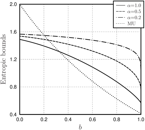
Figure 2: Entropic uncertainty relations as in Fig. 1 for $\measuredangle(\vec{a},\vec{b})=\pi/3$. Note a larger range of parameter $b$ for which majorization bound (27) is stronger than (71).

Majorization relations (23) and (22) lead to uncertainty bounds on the sum of corresponding entropies of the same order. Except for (71), the Maassen–Uffink approach provides a lower bound on the sum of entropies of different orders. Relaxing a restriction, the right-hand side of (71) gives a lower bound on the sum of two Rényi’s entropies of the same order $0<\alpha\leq 1$. It is known that the Rényi $\alpha$-entropy does not increase with growth of the parameter $\alpha$.

We shall now return to our example of two quantum operations with the Kraus operators (61) and (62), respectively. Let us denote

$${\mathsf{P}}_{\pm}=|{\mathsf{A}}_{\pm}|^{2}\ ,\qquad{\mathsf{Q}}_{\pm}=|{\mathsf{B}}_{\pm}|^{2}\ .$$ (72)

One then gives $\bar{f}({\mathcal{P}},{\mathcal{Q}})=c_{1}$ in the sense of (55). Here, we can replace ${\mathsf{A}}_{i}$ and ${\mathsf{B}}_{j}^{\dagger}$ with $|{\mathsf{A}}_{i}|$ and $|{\mathsf{B}}_{j}|$ as the spectral norm is unitarily invariant. Thus, for $0<\alpha\leq 1$ we write

$$H_{\alpha}(p)+H_{\alpha}(q)\geq-2\ln{c}_{1}\ ,$$ (73)

where $p_{\pm}={\mathrm{Tr}}({\mathsf{P}}_{\pm}\boldsymbol{\rho})$ and $q_{\pm}={\mathrm{Tr}}({\mathsf{Q}}_{\pm}\boldsymbol{\rho})$. The inequality (73) is herewith Rényi’s formulation of the Maassen–Uffink type for the example of two qubit channels. Another approach to derive Rényi-entropy uncertainty relations was developed in zbp2014 . We aim to compare (73) with (27), which follows from relation (23) of the direct-sum type.

Let us take two vectors $\vec{a}$ and $\vec{b}$ of the same length $b=|\vec{a}|=|\vec{b}|$. We then write $c_{2}=\sqrt{(1+b)/2}$ and $|\vec{a}\cdot\vec{b}|=b^{2}\cos\measuredangle(\vec{a},\vec{b})$. The result for $c_{1}$ is obtained by substituting the scalar product into the right-hand side of (64). For the given $0<\alpha\leq 1$, the majorization-based entropic bound then follows from (27) by substituting (65). Running $b$, we will visualize the bounds of interest. For two outcomes, the maximal value of (19) is equal to $\ln 2$. It is convenient to rescale Rényi’s entropies by $\ln 2$ so the logarithm becomes taken in the base $2$.

The right-hand side of (27) is shown in Fig. 1 for $\measuredangle(\vec{a},\vec{b})=\pi/2$ and for three values of the parameter $\alpha=1$, $\alpha=0.5$, and $\alpha=0.2$. There is a range of $b$, in which formula (27) gives a stronger bound. At the same time, the Maassen–Uffink bound is better for small $b$, as the probability distributions become almost uniform. In Fig. 2, the right-hand side of (27) is shown for $\measuredangle(\vec{a},\vec{b})=\pi/3$. In this case the range of parameter, for which the bound (27) is stronger becomes greater and the difference between both bounds becomes larger. On the other hand, the Maassen–Uffink bound is still better for sufficiently small $b$. With further decrease of the angle $\measuredangle(\vec{a},\vec{b})$, the picture is similar to this shown in Fig. 2. For sufficiently large $b$, relation (27) provides a significant improvement with respect to the the Maassen–Uffink relation.

VI Equivalence in the case of two orthonormal bases

In this section, we show that the presented formulation of majorization uncertainty relations includes earlier results of prz13 ; rpz14 as particular cases. Let us begin by simplifying the above example of qubit channels with the Kraus operators (61) and (62). The case of two orthonormal bases is realized with two projective measurements of a qubit. To avoid a confusing notation, the corresponding unit vectors will be denoted by $\vec{m}$ and $\vec{n}$. Instead of the Kraus operators (61) and (62), we now deal with rank-one projectors

$${\mathsf{\Pi}}_{\pm} =|e_{\pm}\rangle\langle{e}_{\pm}|=\frac{1}{2}\,\bigl{(}\openone_{2}\pm\vec{m}\cdot\vec{\boldsymbol{\tau}}\bigr{)}\,,$$ (74)

$${\mathsf{\Lambda}}_{\pm} =|f_{\pm}\rangle\langle{f}_{\pm}|=\frac{1}{2}\,\bigl{(}\openone_{2}\pm\vec{n}\cdot\vec{\boldsymbol{\tau}}\bigr{)}\,.$$ (75)

Here, the vectors of each bases are numbered in the “plus/minus” notation. For $i,j=\pm 1$, simple calculations give

$${\mathrm{Tr}}({\mathsf{\Pi}}_{i}{\mathsf{\Lambda}}_{j})=\bigl{|}\langle{e}_{i}|f_{j}\rangle\bigr{|}^{2}=\frac{1+ij{\,}\vec{m}\cdot\vec{n}}{2}\ .$$ (76)

In our example, the formulas (64) and (76) lead to the same result, since

$$s_{1}=\underset{ij}{\max}\bigl{|}\langle{e}_{i}|f_{j}\rangle\bigr{|}=\sqrt{\frac{1+|\vec{m}\cdot\vec{n}|}{2}}=c_{1}\ .$$ (77)

In the case considered, the formula (63) further gives $c_{2}=1$. From (8), we obtain the same value. Indeed, the quantity $s_{2}$ is the maximum among the spectral norms of the matrices

$$\begin{pmatrix}\langle{e}_{i}|f_{+}\rangle&\langle{e}_{i}|f_{-}\rangle\end{pmatrix}\,,\qquad\begin{pmatrix}\langle{e}_{+}|f_{j}\rangle\\ \langle{e}_{-}|f_{j}\rangle\end{pmatrix}\,.$$ (78)

In two dimensions, the spectral norm of each of the matrices (78) is equal to $1$. It follows from the completeness relation. As noted in (57), we have $c_{3}=1$. The spectral norm of a unitary matrix is also $1$, so that $s_{3}=1$. For two rank-one projective measurements of a qubit, more general approach of Section IV leads to the same majorization relations as the previous formulation proposed in prz13 ; rpz14 .

We shall now prove the above claim for an arbitrary finite dimensionality. In such general case, we will assume that the basis vectors are numbered by the index running from $1$ to $d$. The precise statement is formulated as follows.

Proposition 6

Let $\{|e_{i}\rangle\}$ and $\{|f_{j}\rangle\}$ be two orthonormal bases in $d$-dimensional Hilbert space. In terms of the rank-one projectors

$${\mathsf{\Pi}}_{i}=|e_{i}\rangle\langle{e}_{i}|\ ,\qquad{\mathsf{\Lambda}}_{j}=|f_{j}\rangle\langle{f}_{j}|\ ,$$ (79)

we define the sequence of positive numbers

$$c_{k}:=\max\!\left\{\|{\mathsf{Z}}\|_{\infty}:{\>}{\mathsf{Z}}\in\mathcal{BSUB}\bigl{(}{\mathsf{C}}_{{\mathsf{\Pi}}{d}}{\mathsf{C}}_{{\mathsf{\Lambda}}{d}}^{\dagger}{\,},k\bigr{)}\right\}\,.$$ (80)

For all $k=1,\ldots,d$, we then have $c_{k}=s_{k}$, where $s_{k}$ is defined by (8) with the unitary matrix ${\mathsf{W}}=\bigl{[}\bigl{[}\langle{e}_{i}|f_{j}\rangle\bigr{]}\bigr{]}$.

Proof. Let ${\mathsf{U}}_{e}$ and ${\mathsf{U}}_{f}$ be the two unitary transformations such that

$${\mathsf{U}}_{e}{\,}|e_{i}\rangle=|i\rangle\ ,\qquad{\mathsf{U}}_{f}{\,}|f_{j}\rangle=|j\rangle\ .$$ (81)

By $|i\rangle\in\mathbb{M}_{d\times 1}(\mathbb{C})$, we mean the column with $1$ on $i$-th place and with $0$ on all the other places. That is, the above transformations respectively turn our bases into the computational one. For all $m\in\{1,\ldots,d\}$, we now write

$$\bigl{(}\openone_{m}\otimes{\mathsf{U}}_{e}\bigr{)}{\,}{\mathsf{C}}_{{\mathsf{\Pi}}{m}}={\mathrm{diag}}\underset{\text{$m$ blocks}}{\underbrace{({\mathsf{U}}_{e},\ldots,{\mathsf{U}}_{e})}}\begin{pmatrix}{\mathsf{\Pi}}_{1}\\ \ldots\\ {\mathsf{\Pi}}_{m}\end{pmatrix}=\begin{pmatrix}|1\rangle\langle{e}_{1}|\\ \ldots\\ |m\rangle\langle{e}_{m}|\end{pmatrix}.$$ (82)

Similarly, the block column $\bigl{(}\openone_{n}\otimes{\mathsf{U}}_{f}\bigr{)}{\,}{\mathsf{C}}_{{\mathsf{\Lambda}}{n}}$ is represented. As the spectral norm is unitarily invariant, for all $m,n\in\{1,\ldots,d\}$ we have

$$\bigl{\|}{\mathsf{C}}_{{\mathsf{\Pi}}{m}}{\mathsf{C}}_{{\mathsf{\Lambda}}{n}}^{\dagger}\bigr{\|}_{\infty}=\left\|\bigl{(}\openone_{m}\otimes{\mathsf{U}}_{e}\bigr{)}{\,}{\mathsf{C}}_{{\mathsf{\Pi}}{m}}{\mathsf{C}}_{{\mathsf{\Lambda}}{n}}^{\dagger}{\,}\bigl{(}\openone_{n}\otimes{\mathsf{U}}_{f}^{\dagger}\bigr{)}\right\|_{\infty}\,.$$ (83)

Therefore, the numbers of the form (80) can be calculated by replacing ${\mathsf{C}}_{{\mathsf{\Pi}}{d}}{\mathsf{C}}_{{\mathsf{\Lambda}}{d}\,}^{\dagger}$ with the block matrix

$$\widetilde{{\mathsf{W}}}:=\bigl{(}\openone_{d}\otimes{\mathsf{U}}_{e}\bigr{)}{\,}{\mathsf{C}}_{{\mathsf{\Pi}}{d}}{\mathsf{C}}_{{\mathsf{\Lambda}}{d}}^{\dagger}{\,}\bigl{(}\openone_{d}\otimes{\mathsf{U}}_{f}^{\dagger}\bigr{)}\,.$$ (84)

It follows from (82) that the $(i,j)$-block of $\widetilde{{\mathsf{W}}}$ is the $d\times{d}$ matrix $w_{ij}{\,}|i\rangle\langle{j}|$. Due to the structure of the computational basis, the $(i,j)$-entry of this block reads $w_{ij}=\langle{e}_{i}|f_{j}\rangle$, while all other entries are equal zero.

To each block $m\times{n}$ submatrix of $\widetilde{{\mathsf{W}}}$, we assign the $m\times{n}$ submatrix of ${\mathsf{W}}$. The latter is obtained from the former by replacing each $d\times{d}$ block $w_{ij}{\,}|i\rangle\langle{j}|$ by the single entry $w_{ij}$. Such a replacement implies that we eliminate some purely zero rows and columns from the submatrix of blocks. Due to Lemma 1, this operation does not alter the spectral norm. Thus, there is one-to-one correspondence between block submatrices of $\widetilde{{\mathsf{W}}}$ and usual submatrices of ${\mathsf{W}}$ with the following property. It provides the same value of the spectral norms of an element of $\mathcal{BSUB}\bigl{(}\widetilde{{\mathsf{W}}},k\bigr{)}$ and its “twin” of $\mathcal{SUB}({\mathsf{W}},k)$. For any given $k=1,\ldots,d$ we actually deal with the same collection of values of the spectral norm of an element. Hence, the optimization of (80) results in $c_{k}=s_{k}$, where the latter quantity is defined by (8). $\blacksquare$

The statement of Proposition 6 justifies that the approach of Sect. IV is a natural and reasonable extension of the formulations of the papers prz13 ; rpz14 . In the case of two orthonormal bases, the sequence of numbers $c_{k}$ is actually reduced to the sequence of numbers $s_{k}$ defined by (8). This fact was also exemplified in Sec. V with the one-qubit example.

VII Concluding Remarks

We have derived majorization uncertainty relations for a pair of trace–preserving quantum operations. They are an extension of the previous technique developed in prz13 ; rpz14 . In the case of orthonormal bases, majorization relations were posed in terms of spectral norms of submatrices of a unitary matrix. We have generalized this approach by considering norms of block matrices comprised of the corresponding Kraus operators. To any collection of Kraus operators, we assign a vector of probabilities generated by the input state. Majorization relations of both the direct-sum and the tensor-product types are obtained within the developed scheme. The direct-sum majorization relations for orthogonal measurements provide bounds stronger than these obtained with the tensor product of probability vectors rpz14 . This conclusion remains valid also in the considered case of quantum operations.

Existing freedom in the choice of Kraus operators is somehow reflected in the context of uncertainty relations. First of all, this choice has an impact on the probabilities assigned to quantum operations in (30). The right-hand sides of (23) and (22) depend also on the chosen Kraus operators. In this sense, we rather deal with majorization uncertainty relations for given unravelings of quantum operations, each determined by a concrete set of measurement operators.

In this work we analyzed the simplest case of two quantum operations. However, the same approach allows us to get some non-trivial bounds also in the case of a single operation – see A. As was shown in rpz14 , majorization relations of the direct-sum type are naturally reformulated for several measurements in orthonormal bases. Extending such a treatment for the case of several quantum operations remains as a topic of future research.

Entropic majorization relations for two arbitrary quantum operations derived in this work can be considered as a direct generalization of previous results concerning orthogonal measurements prz13 ; rpz14 . Dealing with spectral norms of submatrices, majorization relations of both types can be obtained in a unified way. Presented approach is focused on norms of block submatrices of block matrices comprised of the corresponding Kraus operators.

Although majorization relations derived in this work were illustrated with an explicit example for a pair of trace-preserving completely positive maps acting on a single qubit, they are valid for arbitrary two quantum operations acting on a finite-dimensional state. Therefore these results can be applied for studying various problems in the theory of quantum information.

As entropic uncertainty relations represent lower bounds for the average entropy characterizing a given measurement, one studies also so-called entropic certainty relations sanchez93 , i.e. the corresponding upper bounds. Although for two orthogonal measurements in $d$-dimensional space the trivial upper bound equal to $\log{d}$ is always saturated KLJR14 , some nontrivial certainty relations for three or more orthogonal measurements were recently derived in PRCPZ15 . It would be therefore interesting to study an analogous problem for quantum operations. To be more specific, one can pose the problem of finding upper bounds for the average entropy characterizing generalized measurements with the number of Kraus operators equal to the rank of the Choi matrices corresponding to the investigated quantum operations.

Appendix A Majorization relations for a single quantum operation

In this section, we present applications of the majorization approach to a single quantum operation. Let the set $\mathcal{A}=\{{\mathsf{A}}_{i}\}$ with $N$ elements be unraveling of a TPCP map $\Phi$. The following statement takes place. For all $m\in\{1,\ldots,N\}$ and arbitrary density matrix $\boldsymbol{\rho}\in{\mathcal{L}}_{+}(\mathcal{H}_{d})$, we have

$$\sum\nolimits_{i=1}^{m}p_{i}(\mathcal{A}|\boldsymbol{\rho})\leq\|{\mathsf{C}}_{Am}^{\dagger}{\mathsf{C}}_{Am}\|_{\infty}=\|{\mathsf{C}}_{Am}{\mathsf{C}}_{Am}^{\dagger}\|_{\infty}\ .$$ (85)

Here, the block matrix ${\mathsf{C}}_{Am}$ is defined according to (32). Similarly to (34), the result (85) follows from the relation

$$\sum\nolimits_{i=1}^{m}\langle\psi|{\mathsf{A}}_{i}^{\dagger}{\mathsf{A}}_{i}|\psi\rangle\leq\|{\mathsf{C}}_{Am}^{\dagger}{\mathsf{C}}_{Am}\|_{\infty}\ ,$$ (86)

where $|\psi\rangle$ is an arbitrary pure state. Therefore, the vector comprised of probabilities $p_{i}(\mathcal{A}|\boldsymbol{\rho})$ is majorized by the vector

$$\widetilde{\omega}=\bigl{(}\widetilde{c}_{1},\widetilde{c}_{2}-\widetilde{c}_{1},\ldots,\widetilde{c}_{N^{2}-1}-\widetilde{c}_{N^{2}-2}\bigr{)}\ ,$$ (87)

with entries given by the norms

$$\widetilde{c}_{k}:=\max\!\left\{\|{\mathsf{Z}}\|_{\infty}:{\>}{\mathsf{Z}}\in\mathcal{BSUB}\bigl{(}{\mathsf{C}}_{AN}{\mathsf{C}}_{AN}^{\dagger},k\bigr{)}\right\},$$ (88)

were notation introduced in (10) is used. Note that for any $k>1$ the norms are non-decreasing, $c_{k}\geq c_{k-1}$, so that the entries of the vector $\widetilde{\omega}$ are non-negative. The completeness relation can be reexpressed as ${\mathsf{C}}_{AN}^{\dagger}{\mathsf{C}}_{AN}=\openone_{d}\,$, whence we always have

$$\widetilde{c}_{N^{2}-1}=\|{\mathsf{C}}_{AN}{\mathsf{C}}_{AN}^{\dagger}\|_{\infty}=\|{\mathsf{C}}_{AN}^{\dagger}{\mathsf{C}}_{AN}\|_{\infty}=1\ .$$ (89)

Since the Rényi and Tsallis entropies are both Schur concave, the following inequalities follow for all $\alpha>0$,

$$H_{\alpha}(p) \geq{H}_{\alpha}\bigl{(}\widetilde{\omega}\bigr{)}\ ,$$ (90)

$$T_{\alpha}(p) \geq{T}_{\alpha}\bigl{(}\widetilde{\omega}\bigr{)}\ .$$ (91)

Let us illustrate these entropic relations with the following example. Consider four Kraus operators acting on a single-qubit system,

$${\mathsf{A}}_{1}=\begin{pmatrix}0&\sqrt{a}\\ 0&0\end{pmatrix}, {\mathsf{A}}_{2}=\begin{pmatrix}0&0\\ \sqrt{b}&0\end{pmatrix},$$ (92)

$${\mathsf{A}}_{3}={\mathrm{diag}}\bigl{(}0,\sqrt{1-a}\bigr{)}\ , {\mathsf{A}}_{4}={\mathrm{diag}}\bigl{(}\sqrt{1-b},0\bigr{)}\ ,$$ (93)

where real numbers $a$ and $b$ obey $0\leq{a},b\leq 1$. Note that these Kraus operators form a canonical decomposition bengtsson of the quantum operation, as they are mutually orthogonal, ${\mathrm{Tr}}({\mathsf{A}}_{i}{\mathsf{A}}_{j})=0$ for $i\neq{j}$. For $a=b=1/2$ the map reduces to the completely depolarizing channel. Formula (89) gives $\widetilde{c}_{15}=1$. However, the above example at once leads to $\widetilde{c}_{2}=1$. The latter can be seen from relations

$${\mathsf{A}}_{1}^{\dagger}{\mathsf{A}}_{1}+{\mathsf{A}}_{3}^{\dagger}{\mathsf{A}}_{3}={\mathrm{diag}}(0,1)\ ,\qquad{\mathsf{A}}_{2}^{\dagger}{\mathsf{A}}_{2}+{\mathsf{A}}_{4}^{\dagger}{\mathsf{A}}_{4}={\mathrm{diag}}(1,0)\ .$$ (94)

It is sufficient to use the vector $\widetilde{\omega}=\bigl{(}\widetilde{c}_{1},1-\widetilde{c}_{1}\bigr{)}$, whose first element

$$\widetilde{c}_{1}=\max\bigl{\{}a,1-a,b,1-b\bigr{\}}\>.$$ (95)

Here, we generally deal with the four particular probabilities. For this unraveling, Rényi’s $\alpha$-entropy is bounded from below by the binary entropy $H_{\alpha}\bigl{(}\widetilde{c}_{1},1-\widetilde{c}_{1}\bigr{)}$, and Tsallis’ $\alpha$-entropy is bounded from below by the binary entropy $T_{\alpha}\bigl{(}\widetilde{c}_{1},1-\widetilde{c}_{1}\bigr{)}$. In general, such bounds seem not to be very tight. If $a$ and $b$ are both close to $1/2$, the binary entropy is close to the maximal value. Let the input state be such that only two of the four probabilities are significant. Then the above majorization relations provide rather precise bounds. It would be interesting to compare majorization relations with trade-off relations for a single quantum operation. Trade-off relations for a single quantum operation were proposed in rprz12 and later extended in rast13a .

References

- (1) Heisenberg W 1927 Zeitschrift für Physik 43 172
- (2) Busch P, Heinonen T, and Lahti P J 2007 Phys. Rep. 452 155
- (3) Hall M J W 1999 Phys. Rev. A 59 2602
- (4) Robertson H P 1929 Phys. Rev. 34 163
- (5) Maassen H and Uffink J B M 1988 Phys. Rev. Lett. 60 1103
- (6) Zimba J 2000 Found. Phys. 30 179
- (7) Wehner S and Winter A 2010 New. J. Phys. 12, 025009
- (8) I. Białynicki-Birula and Ł. Rudnicki 2011 Entropic uncertainty relations in quantum physics Statistical Complexity (Berlin: Springer) pp 1–34
- (9) Coles P J, Berta M, Tomamichel M, and Wehner S 2015 Entropic uncertainty relations and their applications arXiv:1511.04857 [quant-ph]
- (10) Hirschman I I 1957 Amer. J. Math. 79 152
- (11) Beckner W 1975 Ann. Math. 102 159
- (12) Białynicki-Birula I and Mycielski J 1975 Commun. Math. Phys. 44 129
- (13) Deutsch D 1983 Phys. Rev. Lett. 50 631
- (14) Kraus K 1987 Phys. Rev. D 35 3070
- (15) Ivanovic I D 1995 J. Phys. A: Math. Gen. 25 L363
- (16) Sánchez J 1993 Phys. Lett. A 173 233
- (17) Wu S, Yu S, and Mølmer K 2009 Phys. Rev. A 79 022320
- (18) Rastegin A E 2013 Eur. Phys. J. D 67 269
- (19) Berta M, Christandl M, Colbeck R, Renes J M, and Renner R 2010 Nature Phys. 6 659
- (20) Coles P J and Piani M 2014 Phys. Rev. A 89 022112
- (21) Oppenheim J and Wehner S 2010 Science 330 1072
- (22) Ren L-H and Fan H 2014 Phys. Rev. A 90 052110
- (23) Rastegin A E 2015 Quantum Inf. Process. 14 783
- (24) Rudnicki Ł 2015 Phys. Rev. A 91 032123
- (25) Partovi M H 2011 Phys. Rev. A 84 052117
- (26) Puchała Z, Rudnicki Ł, and Życzkowski K 2013 J. Phys. A: Math. Theor. 46 272002
- (27) Friedland S, Gheorghiu V, and Gour G 2013 Phys. Rev. Lett. 111 230401
- (28) Rudnicki Ł, Puchała Z, and Życzkowski K 2014 Phys. Rev. A 89 052115
- (29) Krishna M and Parthasarathy K R 2002 Sankhyā, Ser. A 64 842
- (30) Rastegin A E 2011 J. Phys. A: Math. Theor. 44 095303
- (31) Hiai F and Petz D 2014 Introduction to Matrix Analysis and Applications (Heidelberg: Springer)
- (32) Horn R A and Johnson C R 1990 Matrix Analysis (Cambridge: Cambridge University Press)
- (33) Watrous J 2015 Theory of Quantum Information a draft of book (Waterloo: University of Waterloo) http://www.cs.uwaterloo.ca/~watrous/TQI/
- (34) Bhatia R 2007 Positive Definite Matrices (Princeton: Princeton University Press)
- (35) Nielsen M A and Chuang I L 2000 Quantum Computation and Quantum Information (Cambridge: Cambridge University Press)
- (36) Bengtsson I and Życzkowski K 2006 Geometry of Quantum States: An Introduction to Quantum Entanglement (Cambridge: Cambridge University Press)
- (37) Carmichael H J 1993 An Open Systems Approach to Quantum Optics (Lecture Notes in Physics vol 18) (Berlin: Springer)
- (38) Rényi A 1961 On measures of entropy and information Proc. 4th Berkeley Symposium on Mathematical Statistics and Probability (Berkeley, CA: University of California Press) pp 547–61
- (39) Müller-Lennert M, Dupuis F, Szehr O, Fehr S, and Tomamichel M 2013 J. Math. Phys. 54 122203
- (40) Berta M, Seshadreesan K P, and Wilde M M 2015 Phys. Rev. A 91 022333
- (41) Tsallis C 1988 J. Stat. Phys. 52 479
- (42) Rajagopal A K, Sudha, Nayak A S, and Usha Devi A R 2014 Phys. Rev. A 89 012331
- (43) Rastegin A E 2015 Ann. Phys. 355 241
- (44) Rastegin A E 2016 Phys. Rev. A 93 032136
- (45) Hall M J W 1997 Phys. Rev. A 55 100
- (46) Białynicki-Birula I 2006 Phys. Rev. A 74 052101
- (47) Massar S 2007 Phys. Rev. A 76 042114
- (48) Rastegin A E 2010 J. Phys. A: Math. Theor. 43 155302
- (49) Hardy G H, Littlewood J E, and Polya G 1934 Inequalities (London: Cambridge University Press)
- (50) Coles P J, Colbeck R, Yu L, and Zwolak M 2012 Phys. Rev. Lett. 108 210405
- (51) Zozor S, Bosyk G M, and Portesi M 2014 J. Phys. A: Math. Theor. 47 495302
- (52) Korzekwa K, Lostaglio M, Jennings D, and Rudolph T 2014 Phys Rev. A 89 042122
- (53) Puchała Z, Rudnicki Ł, Chabuda K, Paraniak M, and Życzkowski K 2015 Phys Rev. A 92 032109
- (54) Roga W, Puchała Z, Rudnicki Ł, and Życzkowski K 2013 Phys Rev. A 87 032308
- (55) Rastegin A E 2013 J. Phys. A: Math. Theor. 46 285301