Applications of the Feynman-Hellmann theorem in hadron structure

Abstract:

The Feynman-Hellmann (FH) relation offers an alternative way of accessing hadronic matrix elements through artificial modifications to the QCD Lagrangian. In particular, a FH-motivated method provides a new approach to calculations of disconnected contributions to matrix elements and high-momentum nucleon and pion form factors. Here we present results for the total nucleon axial charge, including a statistically significant non-negative total disconnected quark contribution of around $-5\%$ at an unphysically heavy pion mass. Extending the FH relation to finite-momentum transfers, we also present calculations of the pion and nucleon electromagnetic form factors up to momentum transfers of around 7–8 GeV². Results for the nucleon are not able to confirm the existence of a sign change for the ratio $\frac{G_{E}}{G_{M}}$, but suggest that future calculations at lighter pion masses will provide fascinating insight into this behaviour at large momentum transfers.

ADP-15-42/T944
DESY 15-214
Edinburgh 2015/28
LTH 1067

1 Introduction

In recent years, lattice calculations have seen much success in reproducing the hadron spectrum, with increasing levels of precision. However with regards to investigations of hadron structure, there are still many outstanding issues that have yet to be fully dealt with. In particular, open questions include the details of the origin of hadronic spin and the short-distance distribution of charge within hadrons.

In 1987, results obtained by the European Muon Collaboration (EMC) [1] (and more recently COMPASS [2]) showed that the quark spin degrees of freedom carry only a small fraction of the overall nucleon spin. Since then, a huge effort has been expended to reproduce this result theoretically, with lattice playing an important role. One challenge in lattice calculations of the nucleon axial matrix elements is the difficulty of accessing fermion line disconnected contributions. There has been significant progress in this area, with the use of stochastic methods to attempt calculations of these quantities [3, 4, 5, 6, 7] (also [8] for the vector matrix element). However in addition to this, there is still much ongoing discussion regarding the need to control potential excited-state contamination effects in three-point function calculations of the connected contributions [9, 10, 11, 12].

Experimental determinations of high-momentum form factors for the nucleon and pion are difficult due to the lack of free neutron or pion targets. The Rosenbluth separation method also has trouble isolating the electric form factor of the proton at high momenta. In lattice, it is difficult to extract clean signals for the vector matrix element from the noise introduced by large momentum projections. Additionally, lattice studies must address the same issues of excited-state contamination control and disconnected contributions as in the axial case.

Recently we have carried out work using a Feynman-Hellmann (FH) motivated method to address some of these issues. This approach uses the FH theorem to calculate hadronic matrix elements in lattice QCD through modifications to the QCD Lagrangian. The method has already seen great success in calculations of connected contributions to axial matrix elements [13], gluon observables [14], and singlet renormalisation factors [15]. Here we show recent determinations of the disconnected contributions to nucleon spin (discussed in detail in [16]), and present preliminary new results for the nucleon and pion electromagnetic form factors.

2 Feynman-Hellmann Methods

The FH method relates shifts in the hadron spectrum, as an external field is applied, to hadronic matrix elements. In this way, it allows quantities traditionally accessed using 3-point functions to be calculated from 2-point functions alone. With an additional operator in the QCD Lagrangian,

$$\mathcal{L}\to\mathcal{L}+\lambda\mathcal{O}\,,$$ (1)

we have (up to choices of correlator projectors for states with non-trivial Dirac structure),

$$\left.\frac{\partial E}{\partial\lambda}\right|_{\lambda=0}=\frac{1}{2E}\langle\,H\,|\,\mathcal{O}(0)\,|\,H\,\rangle\,,$$ (2)

for any hadron state $H$. Hence we see that on the lattice, a particular hadronic matrix element may be calculated by performing hadron spectroscopy for multiple values of $\lambda$, and observing the linear behaviour in the resulting energy shifts about $\lambda=0$.

The modification in Eq. (1) may be made either during gauge field generation, or during the inversion of the Dirac operator matrix. The first case necessitates the generation of new field ensembles for several values of $\lambda$, for each operator, and accesses fermion line disconnected contributions to the matrix element. The second case makes use of existing ensembles, and accesses fermion line connected contributions.

3 Simulation Details

For this work we use gauge configurations with $2+1$ flavours of non-perturbatively $O(a)$-improved Wilson fermions, where the lattice spacing $a\approx 0.074$ fm is set using a number of singlet quantities [17, 18, 19]. The clover action comprises the tree-level Symanzik improved gluon action together with a stout smeared fermion action, modified for the use of the FH technique [13].

For the disconnected results in Sec. 4 we use ensembles with two sets of hopping parameters, $(\kappa_{l},\kappa_{s})=(0.120900,0.120900)\text{ and }(0.121095,0.120512)$, the first of these corresponding to the SU(3) flavour symmetric point. These both have a lattice volume of $L^{3}\times T=32^{3}\times 64$, and the corresponding pion masses are approximately 470 and 310 MeV respectively (in the $\lambda=0$ limit). The ensembles are generated with the modified quark action described in Eq. (3). For further details of these ensembles, and the simulated values of $\lambda$, see [16].

Two volumes ($L^{3}\times T=24^{3}\times 48\text{ and }32^{3}\times 64$) are used for the form factor calculations in Sec. 5, both with hopping parameters $(\kappa_{l},\kappa_{s})=(0.120900,0.120900)$ corresponding to the SU(3) flavour symmetric point. The ensembles have been generated with an unmodified quark action, with the Dirac matrix modified during propagator calculation instead. We use two different values of $\lambda$, and several different sets of kinematics.

4 Disconnected Calculations

The FH approach offers an alternative technique for accessing disconnected contributions to matrix elements. For an analysis of disconnected contributions to the axial operator, we modify the fermion part of the QCD Lagrangian during gauge field generation such that

$$\mathcal{L}\to\mathcal{L}+\lambda\sum_{q=u,d,s}\bar{q}\gamma_{3}\gamma_{5}q\,.$$ (3)

Note that all three simulated flavours are modified simultaneously. It is expected that the larger combined signal will give a better signal-to-noise ratio than the individual flavour contributions.

With the additional operator in Eq. (1), we expect the FH signal to appear in the imaginary part of the nucleon correlation function. Introducing an additional imaginary factor in Eq. (3) would shift this signal into the real channel, however the resulting operator is not $\gamma_{5}$-Hermitian, and hence introduces a sign problem. The nucleon correlator on the modified ensembles takes the form (to first order in $\lambda$),

$$G_{\pm}(\lambda,t)\xrightarrow{\text{large }t}\left[A\pm\lambda(\Delta A+i\Delta B)\right]e^{-\left[E\pm i\lambda\Delta\Sigma_{\text{disc.}}\right]t}\,,$$ (4)

where the disconnected contribution to the total quark spin fraction

$$\Delta\Sigma_{\text{disc.}}=\Delta u_{\text{disc.}}+\Delta d_{\text{disc.}}+\Delta s\,,$$ (5)

and $\Delta A$ and $\Delta B$ are arbitrary real numbers parameterising the shift in the correlation amplitude. The $\pm$ signs correspond to spin-up and down positive parity projections of the lattice nucleon state respectively. To extract $\Delta\Sigma_{\text{disc.}}$, we form a ratio of correlators on each ensemble, which is approximately linear in $t$ (to first order in $\lambda$) for large lattice times,

$$R(\lambda,t)=\frac{\operatorname{Im}\left[G_{-}(\lambda,t)-G_{+}(\lambda,t)\right]}{\operatorname{Re}\left[G_{-}(\lambda,t)+G_{+}(\lambda,t)\right]}\xrightarrow{\text{large }t}\lambda\Delta\Sigma_{\text{disc.}}t-\lambda\frac{\Delta B}{A}\,.$$ (6)

We introduce an effective phase shift, which at large times indicates ground state saturation,

$$\phi_{\text{eff.}}=\frac{1}{a}\left[R(\lambda,t+a)-R(\lambda,t)\right]\xrightarrow{\text{large }t}\lambda\Delta\Sigma_{\text{disc.}}\,.$$ (7)

Fig. 2 shows the change in the correlator phase with changing $\lambda$ at the SU(3) flavour symmetric point, extracted using the described methods. By fitting the linear dependence of the phase shift, and repeating the analysis at the lighter mass, we calculate the quark disconnected contribution to $\Delta\Sigma$ (renormalised according to determinations of the singlet and non-singlet factors in [15]) of

$$\Delta\Sigma^{\overline{\text{MS}}(2\text{ GeV})}_{\text{disc.}}\;(m_{\pi}\approx 470\text{ MeV}) =-0.055(18)\,,$$ (8)

$$\Delta\Sigma^{\overline{\text{MS}}(2\text{ GeV})}_{\text{disc.}}\;(m_{\pi}\approx 310\text{ MeV}) =\phantom{-}0.026(14)\,.$$ (9)

The result at the heavier mass is consistent with existing results, however the unusual behaviour at the lighter mass remains to be quantified.

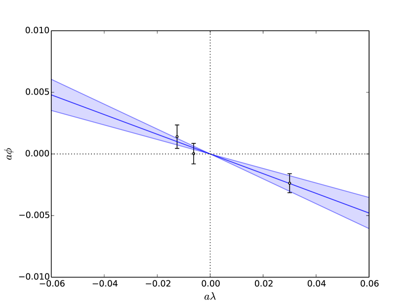
Figure 1: Correlator phase on each ensemble as a function of $\lambda$, with the axial operator term included in the fermion action during gauge field generation with $(\kappa_{l},\kappa_{s})=(0.120900,0.120900)$. The slope is proportional to the quantity $\Delta\Sigma_{\text{disc.}}$

Figure 2: Pion form factor as a function of momentum transfer from both the FH method and JLab experimental data. The vector meson dominance is included to guide the eye.

5 Form Factors

By including a non-zero momentum injection in the operator insertion, we are able to apply the FH approach to calculate more general non-forward matrix elements. We make the modification to the Lagrangian density

$$\mathcal{L}(x)\to\mathcal{L}(x)+\lambda e^{i\vec{q}\cdot(\vec{x}-\vec{x_{0}})}\bar{q}(x)\gamma_{\mu}q(x)\,,$$ (10)

where the modification is made to the $u$ and $d$ quarks separately. This change is only applied to the Dirac fermion operator before inversion, and hence we only access connected contributions to the vector matrix element. Note that the momentum insertion is made with respect to some spatial location $\vec{x}_{0}$, and hence we restrict the space source location for quark propagators to this point. Our application of the FH relation requires momentum projection at the propagator sink to enforce Breit frame kinematics. This choice acts to avoid an energy transfer through the current, which would lead to a non-trivial time dependence of the correlation function.

We perform the operator insertion in Eq. (10) for two components of the vector current ($\mu=2,4$), and several different momentum transfers. For the majority of the chosen kinematics, the total 3-vector momentum is zero, with $\vec{p}\mkern 2.0mu\vphantom{p}^{\prime}=-\vec{p}$. It is this simple case that is discussed here, with more complicated momentum transfers to be discussed in a future publication. These kinematics, in addition to the Breit frame requirement, allow us to minimise momentum projection at the propagator sink, which appears to reduce the noise introduced to the correlation function.

5.1 Pion

Individual quark contributions to the pion vector form factor $F_{\pi}$ are given by

$$\langle\,\pi(\vec{p}\mkern 2.0mu\vphantom{p}^{\prime})\,|\,\bar{q}(0)\gamma_{\mu}q(0)\,|\,\pi(\vec{p})\,\rangle=(p_{\mu}+p_{\mu}^{\prime})F_{\pi q}(Q^{2})\,.$$ (11)

Note that we work in the isospin symmetric limit, and consider only the modification to the $u$ quark in the $\pi^{+}$ state. The $d$ quark result comes from charge conjugation. With the modification to the Lagrangian in Eq. (10), considering only the temporal component of the vector current, we have

$$\left.\frac{\partial E}{\partial\lambda}\right|_{\lambda=0}=F_{\pi}(Q^{2})\,.$$ (12)

For the spatial component of the vector current, the first order shift in the energy vanishes when $\vec{p}\mkern 2.0mu\vphantom{p}^{\prime}+\vec{p}=\vec{0}$, and so we only use results from the temporal current insertion.

Fig. 2 shows results obtained for $Q^{2}F_{\pi}(Q^{2})$ at a variety of momentum transfers, compared with experimental data from JLab. The form factor is anticipated to be quite sensitive to the quark mass, however the overall trend is in good agreement with naive vector meson dominance. A discussion of the asymptotic transition in the context of [20] will feature in an upcoming publication. Included on the plot are the $Q^{2}$ targets for the JLab upgrade, and expected error ranges. We note that lattice results at such large momenta may be particularly complimentary to such experiments.

5.2 Nucleon

Individual quark contributions to the Dirac and Pauli form factors ($F_{1}$ and $F_{2}$ respectively) for the nucleon are defined by the matrix elements

$$\langle\,N(\vec{p}\mkern 2.0mu\vphantom{p}^{\prime},\vec{s}\mkern 2.0mu\vphantom{s}^{\prime})\,|\,\bar{q}(0)\gamma_{\mu}q(0)\,|\,N(\vec{p},\vec{s})\,\rangle=\bar{u}(\vec{p}\mkern 2.0mu\vphantom{p}^{\prime},\vec{s}\mkern 2.0mu\vphantom{s}^{\prime})\left[\gamma_{\mu}F_{1q}(Q^{2})+\sigma_{\mu\nu}\frac{q_{\nu}}{2m}F_{2q}(Q^{2})\right]u(\vec{p},\vec{s})\,.$$ (13)

For the temporal component of the current insertion we choose projection matrices to project unpolarised positive parity states, and for the spatial component we project spin up and down positive parity states individually. The resulting energy shifts from the FH relation are in general linear combinations of $F_{1}$ and $F_{2}$, and the results from both current insertions can be combined to extract the two form factors individually. However for the case $\vec{p}\mkern 2.0mu\vphantom{p}^{\prime}=-\vec{p}$, the FH analysis is greatly simplified. The shifts from the insertion of the temporal and spatial currents are directly proportional to the Sachs electric and magnetic form factors respectively,

$$\left.\frac{\partial E}{\partial\lambda}\right|_{\lambda=0}=\frac{m}{E}G_{Eq}(Q^{2})\qquad\quad\text{and}\quad\qquad\left.\frac{\partial E}{\partial\lambda}\right|_{\lambda=0}=\pm\frac{q_{1}}{2E}G_{M}(Q^{2})\,.$$ (14)

Here $q_{1}$ appears in the spatial case as a result of choosing the second spatial component of the vector current, and the $z$-axis as the spin quantisation axis.

Fig. 3 shows results for the electric and magnetic form factors of the proton, determined by combining results from the individual $u$ and $d$ contributions. We note very good agreement at low $Q^{2}$ between the standard 3-point function method and the FH approach, and particularly draw attention to the very promising results at high $Q^{2}$. Although the current precision is not sufficient to confirm or deny the existence of a zero crossing in the ratio $G_{Ep}/G_{Mp}$, we are optimistic about the possibilities of higher statistics calculations at lighter quark masses.

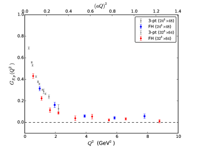
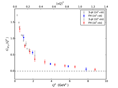
Figure 3: Electric and magnetic form factors for the proton, calculated using the FH method and a standard 3-point function method, on two different lattice sizes.

6 Summary

We have shown how a FH approach can be used to perform a full high-precision calculation of the axial matrix element of the nucleon. We have also shown how the method may be extended to the calculation of non-forward hadron matrix elements. The procedures described may easily be applied to other hadron observables.

Further extensions of the nucleon and pion form factor calculations will attempt to investigate even higher momenta than those already accessed, in addition to explorations of the effect of lattice systematics on such simulations. These will be important for contributing understanding to ongoing experimental efforts to access such scales.

- [1] J. Ashman et al., Phys. Lett. B206, 364 (1988).
- [2] V. Yu. Alexakhin et al., Phys. Lett. B647, 8 (2007), hep-ex/0609038.
- [3] R. Babich et al., Phys. Rev. D85, 054510 (2012), 1012.0562.
- [4] G. S. Bali et al., Phys. Rev. Lett. 108, 222001 (2012), 1112.3354.
- [5] M. Engelhardt, Phys. Rev. D86, 114510 (2012), 1210.0025.
- [6] A. Abdel-Rehim et al., Phys. Rev. D89, 034501 (2014), 1310.6339.
- [7] M. Deka et al., Phys. Rev. D91, 014505 (2015), 1312.4816.
- [8] J. Green et al., Phys. Rev. D92, 031501 (2015), 1505.01803.
- [9] B. J. Owen et al., Phys. Lett. B723, 217 (2013), 1212.4668.
- [10] S. Capitani et al., Phys. Rev. D86, 074502 (2012), 1205.0180.
- [11] S. Dinter et al., Phys. Lett. B704, 89 (2011), 1108.1076.
- [12] T. Bhattacharya et al., Phys. Rev. D89, 094502 (2014), 1306.5435.
- [13] A. J. Chambers et al., Phys. Rev. D90, 014510 (2014), 1405.3019.
- [14] R. Horsley et al., Phys. Lett. B714, 312 (2012), 1205.6410.
- [15] A. J. Chambers et al., Phys. Lett. B740, 30 (2015), 1410.3078.
- [16] A. J. Chambers et al., (2015), 1508.06856.
- [17] V. G. Bornyakov et al., (2015), 1508.05916.
- [18] W. Bietenholz et al., Phys. Lett. B690, 436 (2010), 1003.1114.
- [19] W. Bietenholz et al., Phys. Rev. D84, 054509 (2011), 1102.5300.
- [20] L. Chang et al., Phys. Rev. Lett. 111, 141802 (2013), 1307.0026.
- [21] Y. Nakamura and H. Stüben, PoS LATTICE2010, 040 (2010), 1011.0199.
- [22] P. A. Boyle, Comput. Phys. Commun. 180, 2739 (2009).
- [23] R. G. Edwards and B. Joo, Nucl. Phys. Proc. Suppl. 140, 832 (2005), hep-lat/0409003.