Multiple–Instance Learning: Christoffel Function Approach to Distribution Regression Problem.

Abstract

$Id: DistReg.tex,v 1.53 2015/11/22 23:16:03 mal Exp $

A two–step Christoffel function based solution is proposed to distribution regression problem. On the first step, to model distribution of observations inside a bag, build Christoffel function for each bag of observations. Then, on the second step, build outcome variable Christoffel function, but use the bag’s Christoffel function value at given point as the weight for the bag’s outcome. The approach allows the result to be obtained in closed form and then to be evaluated numerically. While most of existing approaches minimize some kind an error between outcome and prediction, the proposed approach is conceptually different, because it uses Christoffel function for knowledge representation, what is conceptually equivalent working with probabilities only. To receive possible outcomes and their probabilities Gauss quadrature for second–step measure can be built, then the nodes give possible outcomes and normalized weights – outcome probabilities. A library providing numerically stable polynomial basis for these calculations is available, what make the proposed approach practical.

I Introduction

Multiple instance learning is an important Machine Learning (ML) concept having numerous applicationsYang (2005). In multiple instance learning class label is associated not with a single observation, but with a “bag” of observations. A very close problem is distribution regression problem, where a $l$-th sample distribution of $x$ is mapped to a single $y^{(l)}$ value. There are numerous heuristics methods developed from both: ML and distribution regression sides, see Szabó et al. (2014) for review. As in any ML problem the most important part is not so much the learning algorithm, but the way how the learned knowledge is represented. Learned knowledge is often represented as a set of propositional rules, regression function, Neural Network weights, etc. Most of the approaches minimize an error between result and prediction, and some kind of $L^{2}$ metric is often used as an error. The simplest example of such approach is least squares–type approximation. However, there is exist different kind of approximation, Radon–Nikodym type, that operates not with result error, but with sample probabilty, see the Ref. Malyshkin (2015) as an example comparing two these approaches.

Similar transition from result error to probability of outcomes is made in this paper. In this work we use Christoffel function as a mean to store knowledge learned. Christoffel function is a very fundamental concept related to “distribution density”, quadratures weights, number of observations, etcTotik (11 Nov. 2005); Nevai (1986). Recent progress in numerical stability of high order distribution moments calculationMalyshkin and Bakhramov (2015) allows Christoffel function to be built to a very high order, what make practical the approach of using Christoffel function as way to represent knowledge learned.

The paper is organized as following: In Section II a general theory of distribution regression is discussed and close form result, Eq. (10), is presented. Then in Section III numerical example of Eq. (10) application is presented. In Section IV possible further development is discussed.

II Christoffel Function Approach

Consider distribution regression problem where a bag of $N$ observations $x$ is mapped to a single outcome observation $y$ for $l=[1..M]$.

$$(x_{1},x_{2},\dots,x_{j},\dots,x_{N})^{(l)} \to y^{(l)}$$ (1)

A distribution regression problem can have a goal to estimate $y$, average of $y$, distribution of $y$, etc. given specific value of $x$. While the Christoffel function can be used as a proxy to probabilty estimation, but for “true” distribution estimation a complete Gauss quadrature should be built, then the nodes would give possible outcomes and normalized weights – outcome probabilities.

For further development we need $x$ and $y$ bases $Q_{k}(x)$ and $Q_{m}(y)$ and some $x$ and $y$ measure. For simplicity, not reducing the generality of the approach, we are going to assume that $x$ measure is a sum over $j$ index $\sum_{j}$, $y$ measure is a $\sum_{l}$, the basis functions $Q_{k}(x)$ are polynomials $k=0..d_{x}-1$, and $Q_{m}(y)$ are polynomials $m=0..d_{y}-1$ where $d_{x}$ and $d_{y}$ is the number of elements in $x$ and $y$ bases, typical value for $d_{x}$ and $d_{y}$ is below 10–15.

If no $x$ observations exist in each bag ($N=0$), how to estimate the number of observations for given $y$ value? The answer is Christoffel function $\lambda(y)$.

$$G_{y} = <Q_{s}Q_{t}>_{y}=\sum_{l=1}^{M}Q_{s}(y^{(l)})Q_{t}(y^{(l)})$$ (2)

$$K(z,y) = \sum_{s,t=0}^{d_{y}-1}Q_{s}(z)\left(G_{y}\right)^{-1}_{st}Q_{t}(y)$$ (3)

$$\lambda(y) = \frac{1}{K(y,y)}$$ (4)

The $G_{y}$ is Gramm matrix, $K(y,y)$ is a positive quadratic form with matrix equal to Gramm matrix inverse and is a polynomial of $2d_{y}-2$ order, when the form is expanded. The $K(z,y)$ is a reproducing kernel: $P(z)=\sum_{l=1}^{M}K(z,y^{(l)})P(y^{(l)})$ for any polynomial $P$ of degree $d_{y}-1$ or less. For numerical calculations of $K(y,y)$ see Ref. Malyshkin and Bakhramov (2015), Appendix C.

The $\lambda(y)$ define a value similar in nature to “the number of observations”, or “probability”, “weight”, etcTotik (11 Nov. 2005); Nevai (1986). (The equation $M=\sum_{i=0}^{d_{y}-1}\lambda(y_{i})$ holds, when $y_{i}$ correspond to quadrature nodes build on $y$–distribution, the $y_{i}$ are eigenvalues of generalized eigenfunctions problem: $\sum_{t=0}^{d_{y}-1}<yQ_{s}Q_{t}>_{y}\psi_{t}^{(i)}=y_{i}\sum_{t=0}^{d_{y}-1}<Q_{s}Q_{t}>_{y}\psi_{t}^{(i)}$, also note that $\lambda(y_{i})=1/K(y_{i},y_{i})=1/\left(\sum_{t=0}^{d_{y}-1}\psi_{t}^{(i)}Q_{t}(y_{i})\right)^{2}$ and $0=\sum_{t=0}^{d_{y}-1}\psi_{t}^{(s)}Q_{t}(y_{i})$ for $s\neq i$. The asympthotic of $\lambda(y)$ can also serve as important characteristics of distribution propertyTotik (11 Nov. 2005).) The problem now is to modify $\lambda(y)$ to take into account given $x$ value. If, in addition to $y^{(l)}$, we have a vector $x_{j}^{(l)}$ as precondition, then the weight in (2) for each $l$, should be no longer equal to the constant for all terms, but instead, should be calculated based on the number of $x_{j}^{(l)}$ observations that are close to given $x$ value. Let us use Christoffel function once again, but now in $x$–space under fixed $l$ and estimate the weight for $l$-th observation of $y$ as equal to $\lambda^{(l)}(x)$

The result for $\lambda(y|x)$ is:

$$<Q_{k}>^{(l)}_{x} = \sum_{j=1}^{N}Q_{k}(x_{j}^{(l)})$$ (5)

$$G^{(l)} = <Q_{q}Q_{r}>^{(l)}_{x}=\sum_{j=1}^{N}Q_{q}(x_{j}^{(l)})Q_{r}(x_{j}^{(l)})$$ (6)

$$\lambda^{(l)}(x) = \frac{1}{\sum_{k,m=0}^{d_{x}-1}Q_{k}(x)\left(G^{(l)}\right)^{-1}_{km}Q_{m}(x)}$$ (7)

$$<Q_{s}>_{\lambda} = \sum_{l=1}^{M}\lambda^{(l)}(x)Q_{s}(y^{(l)})$$ (8)

$$G_{y|x} = <Q_{s}Q_{t}>_{\lambda}=\sum_{l=1}^{M}\lambda^{(l)}(x)Q_{s}(y^{(l)})Q_{t}(y^{(l)})$$ (9)

$$\lambda(y|x) = \frac{1}{\sum_{s,t=0}^{d_{y}-1}Q_{s}(y)\left(G_{y|x}\right)^{-1}_{st}Q_{t}(y)}$$ (10)

The $\lambda(y|x)$ is the answer. The $G_{y|x}$ is very similar to (2), but now the $l$-th term weight is $\lambda^{(l)}(x)$ instead of a constant. For a given $x$ the (10) is a function of $y$, having the meaning of observations number (or “probability”–like value when scaled). The conceptual difference between regressing the value of $y$ on $x$ and $x$–dependent weights is conceptually similar to the difference between least squares approximation, where observable value is interpolated and Radon–Nikodym type of approximation, where the weights are interpolatedMalyshkin (2015). In Christoffel function approach only the weights, not the values are interpolated, what gives a new turn to distribution regression problem.

For an estimation of possible $y$ outcomes given $x$, this can be done either using the (8) measure and estimating, say, average $y$ and dispersion, or more interesting, build $d_{y}$–point Gauss quadrature using the measure (8), see Ref. Malyshkin and Bakhramov (2015), Appendix B for numerical algorithm, and, for the measure (8), obtain quadrature nodes $y_{i}$ and weights $\lambda(y_{i}|x)$. Then quadrature nodes $y_{i}$ can be treated as possible $y$–outcomes and $\lambda(y_{i}|x)$ can be treated as the weight, corresponding to $y_{i}$ outcome. Normalizing the weights one receive probabilities of each $y_{i}$–outcome given $x$ value. (The quadratures provide superior information about probabilities of each outcome, taking long–tail information into account, but if one, for whatever reason, still need average $y$ value, corresponding to (8) measure, it can be easily obtained from quadrature averaging $y_{i}$ with probabilities $\lambda(y_{i}|x)/\sum_{m=0}^{d_{y}-1}\lambda(y_{m}|x)$ of $y_{i}$ outcome. The result would match exactly sample average of $y$ for the measure (8). Also note that $\sum_{i=0}^{d_{y}-1}\lambda(y_{i}|x)=\sum_{l=1}^{M}\lambda^{(l)}(x)$).

III Numerical Estimation

The major problem of Christoffel function calculation is numerical instability. For given observations all polynomial bases give identical results, but numerical stability of calculations is drastically different, because Gramm matrix condition number depend strongly on basis choice. If $Q_{k}(x)$ and $Q_{m}(y)$ are chosen as orthogonal polynomials with orthogonality measure support matching the $x$ and $y$ support then for discrete measures the Gramm matrix posses a good condition numberBeckermann (1996). The numerical library we developed, seeMalyshkin and Bakhramov (2015) Appendix A, is able to manipulate polynomials in Chebyshev, Legendre, Laguerre and Hermite bases directly, what allows a stable basis to be used and calculate the moments to a very high order, see Ref. Malyshkin (2015) as an example. The distribution regression problem does not require hundreds of moments as in Malyshkin (2015), the $d_{x}$ and $d_{y}$ are typically lower than 10–15 and also should be substantially lower that $N$ and $M$ values respectively. The numerical calculations are typically stable as long as one of four stable bases from Ref. Malyshkin and Bakhramov (2015) is used.

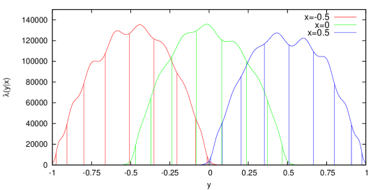
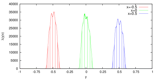
Figure 1: The $\lambda(y|x)$ for $d_{x}=d_{y}=10$ and given $x=\{-0.5,0,0.5\}$ for $R=0.5$ (top) and $R=0.1$ (middle). The $\lambda(y)$ from (4) (bottom). To have $\lambda(y)$ similar to $\lambda(y|x)$ scale it should be multiplied by a factor about $N/d_{x}$. The vertical lines correspond to quadrature built on $\lambda$ – measure, each line height is a weight corresponding to specific outcome.

The algorithm for $\lambda(y|x)$ calculation is this. For each $l$ calculate: $<Q_{k}>^{(l)}_{x}=\sum_{j=1}^{N}Q_{k}(x_{j}^{(l)})$ moments for $k=[0..2d_{x}-1]$, then, using polynomials multiplication operation, from these moments obtain Gramm matrix (6) $G^{(l)}=<Q_{q}Q_{r}>^{(l)}_{x}$ for $q,r=[0..d_{x}-1]$, inverse it and build $\lambda^{(l)}(x)$, a rational function (the nominator is a constant and the denominator is a polynomial of $2d_{x}-2$ order) as in (7), then calculate the $\lambda^{(l)}(x)$ at given value of $x$, save these as the weight for $l$-th observation of $y^{(l)}$. Having the weights, conditional on given $x$ value, calculate $<Q_{m}>_{\lambda}=\sum_{l=1}^{M}\lambda^{(l)}(x)Q_{m}(y^{(l)})$ moments for $m=[0..2d_{y}-1]$, then, using polynomials multiplication operation, from these moments obtain Gramm matrix (9) $G_{y|x}=<Q_{s}Q_{t}>_{\lambda}$ for $s,t=[0..d_{y}-1]$, inverse it and build $\lambda(y|x)$ as in (10). If possible $y$ outcomes and their probabilities are required, then solve generalized eigenvalues problem $\sum_{t=0}^{d_{y}-1}<yQ_{s}Q_{t}>_{\lambda}\psi_{t}^{(i)}=y_{i}\sum_{t=0}^{d_{y}-1}<Q_{s}Q_{t}>_{\lambda}\psi_{t}^{(i)}$, the eigenvalues $y_{i}$ provide possible $y$–outcomes and the weight for each outcome is $\lambda(y_{i}|x)=1/\left(\sum_{t=0}^{d_{y}-1}\psi_{t}^{(i)}Q_{t}(y_{i})\right)^{2}$, the probability of $i$–th outcome is normalized weight $\lambda(y_{i}|x)/\sum_{m=0}^{d_{y}-1}\lambda(y_{m}|x)$ The code performing these calculations is availableMalyshkin (2014), see the file ExampleDistributionDependence.scala.

For application of the algorithm consider the following simple numerical example. Let $y$ be uniformly $[-1\dots 1]$ distributed random variable, $l=[1..M];M=10000$, and for each $y^{(l)}$ generate $j=[1..N];N=1000$ random $x$ as $x=y+R*\epsilon[-1\dots 1]$, where $\epsilon[-1\dots 1]$ is uniformly $[-1\dots 1]$ distributed random variable. Then for given $x$, we want to estimate the distribution of $y$. Let us choose $d_{x}=d_{y}=10$ and plot $\lambda(y|x)$, the function of $y$ for three fixed $x=\{-0.5,0,0.5\}$. In the Fig. 1 we present the chart for $\lambda(y|x)$ for $R=0.5$ and $R=0.1$. Unconditional $\lambda(y)$ from (4) is also presented. (For some applications conditional $\lambda(y|x)/\lambda(y)$ can be also considered).

One can see that the $y$–localization at given $x$ is very clear, and the width of non–vanishing area of $\lambda(y|x)$ track very close the value of randomness parameter $R$. The quadrature built on $\lambda$ measure give both: possible outcomes (quadrature nodes) and weights (outcome probability is normalized weight), presented in the Fig. 1 as vertical lines corresponding to specific $y$–outcome (as we noted above – on quadrature nodes the quadrature weight match exactly Christoffel function value). These calculations can be applied to any kind of distribution, this simple example was used just to demonstrate application of Christoffel function to representation of learned knowledge and to find possible $y$–outcomes and their probabilities.

IV Discussion

In this work a Christoffel function approach to distribution regression problem is proposed. The main idea is to use Christoffel function for knowledge representation. Closed form answer (10) is available. The Christoffel function is used twice: first, to build distribution approximation withing a “bag”, then to model $y$–value distribution of these “bags” using Christoffel function value from the first step as the weight for the observation of $y$. When required, possible $y$ outcomes and their probabilities, can be calculated by building Gauss quadrature instead of using plain Christoffel function answer (10), the quadrature nodes give possible outcomes and normalized quadrature weights give each outcome probability. The method can be extended from real–value to discrete attributes (the $d_{x}$ and $d_{y}$ should be properly adjusted).

The approach, proposed in this paper, as most Multiple–Instance learning approaches, has two stages. The question arise, whether consistent one stage approach exist. For the case $x$ and $y$ being random variables two one–stage interpolation approaches: least squares and Radon–Nikodym have been have been studied in Malyshkin (2015). Now, let us try to find similar one–stage approach, but for random distribution to random variable mapping, same as the (1) problem, we study in this paper. The idea is to convert the problem “random distribution” to “random variable” to the problem “vector of random variables” to “random variable”. The simplest way is to take the moments of random $x$ distribution as “input vector of random variables”. Then least squares and Radon–Nikodym approximations from Malyshkin (2015) can be directly applied. In contrast with the problem (1): given $x$, what can we tell about $y$, this, converted to vector moments problem, would be: given $<Q_{k}>_{x}$ moments of $x$–distribution (fixed $x_{0}$ case can be modeled by $NQ_{k}(x_{0})$), what can we tell about $y$? This problem is solvable in one step. The one–step solution is actually almost identical to 2D problem of image grayscale intensity interpolation we have considered in Malyshkin (2015). There is just one major difference: for image interpolation problem we used basis value at specific point of the raster, but now we would have to use as input the $<Q_{k}>_{x}$ moments of $x$ distribution on which we want to estimate output $y$. The question arise of numerical stability of one–stage method and the problem of data overfitting. While two–stages approach typically effectively have $d_{x}+d_{y}$ elements in basis, the one–stage approach effectively have $d_{x}d_{y}$ elements in basis. By choosing stable basis in Malyshkin (2015) we calculated the moments for $d_{x}=d_{y}=100$ without catching an instability, so basis dimension should not be an issue, but the question of data overfitting for one–stage method require more research and to be published separately. The major advantage of using Christoffel function for knowledge representation is that it stores pure weights, and data overfitting parameter can be estimated as $d_{x}/N$ on first stage and about $d_{y}/M$ on second stage, so in practical applications the problem can be always identified from the beginning.

References

- Yang (2005) Jun Yang, Review of multi-instance learning and its applications, Tech. Rep. (Tech. Rep, 2005).
- Szabó et al. (2014) Zoltán Szabó, Arthur Gretton, Barnabás Póczos, and Bharath Sriperumbudur, “Learning theory for distribution regression,” arXiv preprint arXiv:1411.2066 (2014).
- Malyshkin (2015) Vladislav Gennadievich Malyshkin, “Radon–Nikodym approximation in application to image analysis. http://arxiv.org/abs/1511.01887,” ArXiv e-prints (2015), arXiv:1511.01887 [cs.CV] .
- Totik (11 Nov. 2005) Vilmos Totik, “Orthogonal polynomials,” Surveys in Approximation Theory 1, 70–125 (11 Nov. 2005).
- Nevai (1986) Paul G Nevai, “Géza Freud, Orthogonal Polynomials. Christoffel Functions. A Case Study,” Journal Of Approximation Theory 48, 3–167 (1986).
- Malyshkin and Bakhramov (2015) Vladislav Gennadievich Malyshkin and Ray Bakhramov, “Mathematical Foundations of Realtime Equity Trading. Liquidity Deficit and Market Dynamics. Automated Trading Machines. http://arxiv.org/abs/1510.05510,” ArXiv e-prints (2015), arXiv:1510.05510 [q-fin.CP] .
- Beckermann (1996) Bernhard Beckermann, On the numerical condition of polynomial bases: estimates for the condition number of Vandermonde, Krylov and Hankel matrices, Ph.D. thesis, Habilitationsschrift, Universität Hannover (1996).
- Malyshkin (2014) Vladislav Gennadievich Malyshkin, (2014), the code for polynomials calculation, http://www.ioffe.ru/LNEPS/malyshkin/code.html.