Nonlinear stability of two-dimensional axisymmetric vortices in compressible inviscid medium in a rotating reference frame

Abstract

We study the stability of the vortex in a 2D model of continuous compressible media in a uniformly rotating reference frame. As it is known, the axisymmetric vortex in a fixed reference frame is stable with respect to asymmetric perturbations for the solution of the 2D incompressible Euler equations and basically instable for compressible Euler equations. We show that the situation is quite different for a compressible axisymmetric vortex in a rotating reference frame. First, we consider special solutions with linear profile of velocity (or with spatially-uniform velocity gradients), which are important because many real vortices have similar structure near their centers. We analyze both cyclonic and anticyclonic cases and show that the stability of the solution depends only on the ratio of the vorticity to the Coriolis parameter. Using a very delicate analysis along with computer aided proof, we show that the stability of solutions can take place only for a narrow range of this ratio. Our results imply that the rotation of the coordinate frame can stabilize the compressible vortex. Further, we perform both analytical and numerical analysis of stability for real-shaped vortices.

Keywords: 2D compressible inviscid media, vortex, nonlinear stability, linear profile of velocity

Many flows in oceans and atmospheres are approximately two-dimensional. The vortex structures are their characteristic feature. Two-dimensional vortices also play an important role in tokamak-confined plasmas [61] as well as in astrophysical situations such as accretion discs of neutron stars [28]. Although the vortex dynamics can be complicated, it is natural to begin with the study of certain elementary processes. One example is the stability of isolated circular free vortices in rotating fluids. Their stability/instability properties are of fundamental interest for refined models of general atmospheric circulation due to the presence of strain and shear in the ambient flow.

The vortex motion is traditionally considered in incompressible media. The theory of such motion, going back to the classical works of Helmholtz, Gröbli, Kirchhoff, Rankin, Greenhill, Taylor, Poincaré, has a huge literature (see, e.g. [39], for a modern state-of-art [26], [15], [19] ). Stability of the vortex is the most classical issue. It can be understood in many different ways [35], [15], [57], [21], [31], [29]. Numerical models demonstrate that there is a broad class of geophysical vortices freely evolve toward axisymmetric states. This intrinsic drive toward symmetry opposes the destructive shearing from the environmental flow [55]. Moreover, as it is shown in [53], the axisymmetric form of the vortex is stable with respect to asymmetric perturbations for the two-dimensional inviscid flow.

Nevertheless, the vortex motion in compressible media is also very important both theoretically and practically. Let us show this by example. It is well known that the processes of convergence and divergence of the air flows play an important role in the atmosphere dynamics. Therefore, if we average over the height the original tree-dimensional system of equations for dynamics of the air (using the fact that the horizontal scale is much larger than the vertical one), the resulting two-dimensional model should be compressible in order to reflect the processes.

The earliest results concerning vortices in the compressible fluid were obtained by Chree [16] in the meteorological context. A good review of further works on 2D compressible vortices emphasizing experimental aspects can be found in [6]. In [17], authors present analytical solutions for the reduced system of equations corresponding to free compressible viscous vortices and compare their results with numerical solutions of the full system of equations as well as experiments. In [38], [13], authors discuss different situation of instability in an inviscid compressible media. There exist works, where a linear analysis of stability of compressible vortex was performed in various setting, see [22], [30], [54],[12], [40], [27] and references therein. In [4], [14], [1] steady compressible vortices were constructed using hodograph plane transformations. Mathematical analysis of self-similar isentropic non-rotational 2D Euler system including shock wave structure can be found in [65], see also references therein. In particular, there a non-steady solution corresponding to axisymmetric vortex was obtained.

In the present paper we study the effects of compressibility for a special class of solution of the Euler equations given on a plane rotating with a constant angular velocity. This is a class of solution with spatially-uniform velocity gradients known from Kirchhoff. This class of solution has many outstanding applications, for example, the flow of an ideal homogeneous incompressible fluid inside a triaxial ellipsoid [33], the theory of the motions of solids with cavities filled with a fluid, and the theory of fluid gyroscopes in the field of Coriolis forces [19].

In the incompressible case the Kirchhoff vortex is known to be an analytical solution of the two-dimensional Euler equations (see [33]). This vortex shows a steady rotation without changing its shape. This solution provides a possibility for constructing the vortex patch.

We consider the solution with spatially-uniform velocity gradients for isentropic compressible Euler equations in a rotating coordinate frame. In this case, the only possible ”Kirchhoff vortex” with constant vorticity $\omega$ is axisymmetric vortex. Its nonlinear stability within the class of asymmetric motion having spatially-uniform velocity gradients is under consideration. The elliptical patch does not demonstrate solid body rotation anymore: behavior of the trajectories becomes very complicated.

As in the theory of fluid gyroscopes, the problem is reduced to a study of stability of equilibrium for a quadratically nonlinear system of ordinary differential equations in a phase space of large dimensions. In particular, a linear analysis shows that on some range of parameter $\omega/l$, where $l$ is the Coriolis parameter, even small break of axial symmetry in the initial data leads to break of stability. The linear analysis does not give an answer for the rest of parameters. The analysis of nonlinear stability is much more complicated. In fact, we prove that in general, (except of a discrete number of resonant parameters) the motion is quasi-periodic and therefore stable in the Lyapunov sense up to the the third order terms in the respective normal form. In other words, we prove the necessary stability condition for the ”stable” region. This ”stable” region includes both cases of cyclonic (low pressure in the center of vortex) and anticyclonic (high pressure in the center of vortex) motions. Moreover, the cyclonic motion can be anticlockwise (normal low) or clockwise (anomalous low). If the parameter $\omega/l$ approaches to the very boundaries of linear unstable cyclonic region, the necessary condition for stability fails, and the resonant values appear in a large amount in the domain of anticlockwise motion. Also, the necessary condition for stability fails when the cyclonic values of parameters switch to the cyclonic values and vice versa. The anticyclonic domain contains many resonant values of the parameter, nevertheless, at other points the necessary condition for stability holds.

The problem considered seems artificial since the structure of real vortices in fluid is much more complicated than we discussed here. Indeed, as it is known from laboratory experiments and from observation of large atmospheric vortices like tropical cyclone [56], the velocity has linear profile near the center of vortex. Moreover, as follows from experiments with 2D transverse compressible vortices, the swirl profile defines a vortex core that rotates almost as a rigid body and decays far from the center. This finding is generally consistent with profiles of incompressible vortices. However, the stability of vortex depends on the spatial decay rate for circular vortex in incompressible fluids (see modified Rayleigh criterion [26]).

We performed a series of numerical experiments with initial data corresponding to elliptical deformation of exact axially symmetric stationary solution to 2D inviscid compressible Euler equations constructed in our previous work [50]. This solution has exponential spatial decay at infinity and was used for modeling a moving tropical cyclone in averaged 2D atmosphere.

In these numerical experiments we investigate the stability of cyclonic and anticyclonic vortices with spatially decaying ”tails” and the relations with theoretical results on stability of the vortices having linear velocity profile. We show that for sufficiently small vorticity, the level lines of the pressure near the center of vortex are approximately elliptic. If the vorticity increases, the picture of level lines is similar to the azimuthal Kelvin–Helmholtz instability as observed by Chomaz et al., see [15]. If the vorticity increases further, the numerical solution demonstrates the formation of shock waves.

The paper is organized as follows. In Sec.1, we introduce a two-dimensional system of PDEs, which follows from compressible isentropic inviscid Euler equations after doing appropriate change of variables. In Sec.2, we introduce a special class of solutions for this system and obtain the system of ODEs governing its behavior. In Sec.3, we consider another class of solutions characterized by conservation of mass and energy and show that these solutions are governed by the same system of ODEs. Then we study the stability of the unique equilibrium of this system that refers to a circular steady vortex. In Sec.4, we analyze some simplification of the full system, where the system can be exactly integrated. In Sec.5, we consider the full system. The linearization at equilibrium gives us the instability domain, however, for the rest of parameters the matrix of linearization has three couples of pure imaginary complex conjugate eigenvalues. Therefore, the linear theory does not answer whether the equilibrium is stable or not. To study nonlinear stability, we use the theory of normal forms and apply the theorem about existence of almost periodic trajectories. Due to the difficulty of algebraic computations, we perform them by the computer algebra system MAPLE. The normal forms are analyzed up to the third order. This gives us a possibility to conclude that the system is unstable both near the boundaries of instability domain and near the points where the cyclonic motion changes to anticyclonic one. For the rest of points, may be except for some discrete values, the necessary condition for the stability holds. Moreover, up to the third order term in the normal form expansion, the sufficient condition for stability holds, too. In Sec.6, we present the results of numeric experiments for localized vortices having linear velocity near their center and spatially decaying at infinity. These experiments show that for sufficiently small vorticity the the results about stability for the special class of solutions with linear profile of velocity can catch the main stability features of real-shaped localized vortex. Moreover, we show analytically the reason why the domains of stability for the real-shaped localized vortex basically cannot coincide with the domain of stability for the vortex with linear profile of velocity for large values of vorticity. In Sec.7, we summarize our results.

1 Bidimensional models of rotating compressible medium

The two-dimensional system of motion of inviscous compressible medium on a rotating plane consists of three equations for density $\varrho(t,x),$ velocity ${\bf U}(t,x)$ and pressure $p(t,x)$:

$$\varrho(\partial_{t}{\bf U}+({\bf U}\cdot\nabla){\bf U}+{\mathcal{L}}{\bf U})+\nabla p=0,$$ (1)

$$\partial_{t}\varrho+{\rm div}(\varrho{\bf U})=0,$$ (2)

$$\partial_{t}p+({\bf U}\cdot\nabla p)+\gamma p\,{\rm div}{\bf U}=0.$$ (3)

Here $\mathcal{L}=lL$, $\quad L=\left(\begin{array}[]{cr}0&-1\\ 1&0\end{array}\right)$, $\gamma\in(1,2)$ is the heat ratio, $l>0$ is the Coriolis parameter. $\nabla$ and $\bf\rm div$ denote the gradient and divergence with respect to the space variables. $(.\,\cdot\,.)$ is the inner product. Under suitable boundary conditions, the system (1) – (3) implies conservation of mass, momentum and total energy.

If we restrict ourselves to the barotropic case, where $p=C\rho^{\gamma},\,C={\rm const}$, then the system under consideration can be reduced to two equations (1), (2).

In our previous papers [49], [50], we studied this model in the context of atmosphere dynamics. We started from the (primitive) three-dimensional system of equations for compressible rotating Newtonian polytropic gas [34], [45] and apply the procedure of averaging over the height to obtain a two-dimensional system of equations (see [42]). The vortices in this model were associated with typhoons. In this paper, we do not specify the two-dimensional compressible medium. The results can be applied to other model, nevertheless, our main interest is a possibility of existence of long living atmospherical vortices, therefore in numerical experiments we use the parameters related to the atmosphere.

It will be convenient for us to introduce a new variable $\Pi=p^{\frac{\gamma-1}{\gamma}}$ and reduce (1), (2) to

$$\partial_{t}{\bf U}+({\bf U}\cdot\nabla){\bf U}+{\mathcal{L}}\,{\bf U}+c_{0}\,\nabla\Pi=0,$$ (4)

$$\partial_{t}\Pi+(\nabla\Pi\cdot{\bf U})+(\gamma-1)\,\Pi\,{\rm div}\,{\bf U}=\,0,$$ (5)

$c_{0}=\frac{\gamma}{\gamma-1}C^{\frac{1}{\gamma}}.$

2 A class of exact solutions

Let us look for the solution of (4), (5) in the form

$${\bf U}(t,{\bf x})=Q{\bf x},\qquad Q=\left(\begin{array}[]{cr}a(t)&b(t)\\ c(t)&d(t)\end{array}\right),$$ (6)

$$\Pi(t,{\bf x})=A(t)x_{1}^{2}+B(t)x_{1}x_{2}+C(t)x_{2}^{2}+K(t).$$ (7)

In fact, the solution is the first term of the Taylor series expansion at the point of minimum or maximum of pressure: the first and second term represent velocity and pressure respectively. In this way, we can keep a maximum possible members in this expansion to obtain an exact solution of (4) and (5).

Thus, we get a closed ODE system for the components of the matrices $Q$ and $R=\left(\begin{array}[]{cr}A(t)&\frac{1}{2}B(t)\\ \frac{1}{2}B(t)&C(t),\end{array}\right)$:

$$\dot{R}+RQ+Q^{T}R+(\gamma-1){\bf tr}QR=0,$$ (8)

$$\dot{Q}+Q^{2}+lLQ+2c_{0}R=0,$$ (9)

$$\dot{K}+2(\gamma-1){\bf tr}QK=0.$$

The last equation is linear with respect to $K$, whereas the system of matrix equations (8), (9) consists of 7 nonlinear ODEs and has a very complicated behavior.

In fact, an analogous class of solutions was considered in [5] in another context (see also [59]).

3 Solutions with a finite mass

System (8), (9) can also be applied to describe a behavior of a finite mass of compressible media in non-polytropic case (see [52] and references therein).

Let us recall briefly the derivation. For smooth solutions to (1)-(3), we consider the integrals of total mass ${\cal M}=\int\limits_{{\mathbb{R}}^{2}}\rho d{x}$ and total energy ${{\cal E}}(t)=\int\limits_{{\mathbb{R}}^{2}}\left(\frac{\rho|{\bf U}|^{2})}{2}+\frac{p}{\gamma-1}\right)\,d{x}={\cal E}_{k}(t)+{\cal E}_{p}(t)$. To guarantee the convergence of the integrals, we can assume that the density and pressure vanish as $|{\bf x}|\to\infty$ rather quickly, whereas the velocity components may even grow. For these solutions, the total mass and total energy are conserved. Further, we introduce the following functionals:

$$G(t)=\frac{1}{2}\int\limits_{{\mathbb{R}}^{2}}\rho|{\bf x}|^{2}\,d{x},\quad F_{i}(t)=\int\limits_{{\mathbb{R}}^{2}}({\bf U,X}_{i})\rho\,d{x}$$

and

$$G_{x_{1}}(t)=\frac{1}{2}\int\limits_{{\mathbb{R}}^{2}}\rho x_{1}^{2}d{x},\quad G_{x_{2}}(t)=\frac{1}{2}\int\limits_{{\mathbb{R}}^{2}}\rho x_{2}^{2}d{x},\quad G_{x_{1}x_{2}}(t)=\frac{1}{2}\int\limits_{{\mathbb{R}}^{2}}\rho x_{1}x_{2}\,d{x},$$

where ${\bf X}_{1}=(x_{1},x_{2}),\,{\bf X}_{2}={\bf r}_{\bot}=(x_{2},-x_{1}),$ $\,i=1,2$. We note that for nontrivial solutions $G(t)>0$ and $\Delta(t)=G_{x_{1}}(t)G_{x_{2}}(t)-G_{x_{1}x_{2}}^{2}(t)>0$. It can be readily checked by means of the Green’s formula that for the classical solutions to (1)-(3) the following relations hold:

$$G^{\prime}(t)=F_{1}(t),\quad\quad F_{2}^{\prime}(t)=lF_{1}(t)$$

$$F_{1}^{\prime}(t)=2(\gamma-1){\mathcal{E}}_{p}(t)+2{\mathcal{E}}_{k}(t)-lF_{2}(t),$$

Moreover, for the velocity (6) we have

$$G_{x_{1}}^{\prime}=2aG_{x_{1}}+2bG_{x_{1}x_{2}},\quad G_{x_{2}}^{\prime}=2dG_{x_{2}}+2cG_{x_{1}x_{2}},\quad G_{x_{1}x_{2}}^{\prime}=(a+d)G_{x_{1}x_{2}}+bG_{x_{2}}+cG_{x_{1}},$$

$$E_{p}^{\prime}(t)=-(\gamma-1)(a(t)+d(t))E_{p}(t),\quad\Delta^{\prime}(t)=2(a(t)+d(t))\Delta(t).$$

the potential energy $E_{p}(t)$ is connected with $\Delta(t)$ as follows:

$$E_{p}(t)=E_{p}(0)\Delta^{(\gamma-1)/2}(0)\Delta^{(-\gamma+1)/2}(t).$$

Let us introduce new functions

$$G_{1}(t)={G_{x_{1}}(t)}{\Delta^{-(\gamma+1)/2}(t)},\quad G_{2}(t)={G_{x_{2}}(t)}{\Delta^{-(\gamma+1)/2}(t)},\quad G_{3}(t)={G_{x_{1}x_{2}}}{\Delta^{-(\gamma+1)/2}(t)}.$$

For the elements of the matrix $Q$ and $G_{1},\,G_{2},\,G_{3}$ we get the closed system of equations

$$a^{\prime}=-a^{2}-bc+lc-\mathcal{K}G_{2},$$

$$b^{\prime}=-b(a+d)+ld+\mathcal{K}G_{3},$$

$$c^{\prime}=-c(a+d)-la+\mathcal{K}G_{3},$$

$$d^{\prime}=-d^{2}-bc-lb-\mathcal{K}G_{1},$$

$$G_{1}^{\prime}=((1-\gamma)a-(1+\gamma)d)G_{1}+2bG_{3},$$

$$G_{2}^{\prime}=((1-\gamma)d-(1+\gamma)a)G_{2}+2cG_{3},$$

$$G_{3}^{\prime}=cG_{1}+bG_{2}-\gamma(a+d)G_{3},$$

with $\mathcal{K}=\frac{\gamma-1}{2}E_{p}(0)\Delta^{(\gamma-1)/2}(0).$ The system coincides with (8), (9), where $2c_{0}=\mathcal{K}$, $A=G_{2}$, $B=-2G_{3}$, $C=G_{1}$. Nevertheless, in this case the conservation of the total energy $\mathcal{E}$ implies a supplementary first integral. Moreover, for $\gamma=2$, the explicit form of $F_{1}$ and $F_{2}$ allows to obtain non-autonomous first integrals.

3.1 The case without non inertial forces

In the case $l=0$, the problem about expanding a finite mass of gas in vacuum was studied extendedly in Lagrangian coordinates $\alpha=(\alpha_{1},\alpha_{2})$, where $x(\alpha,t)={\mathcal{F}}(t)\alpha$, ${\mathcal{F}}(t)$ is a square matrix. Thus, $U(x,t)=\dot{x}=\dot{\mathcal{F}}(t){\mathcal{F}}^{-1}(t)x$ and $Q(t)=\dot{\mathcal{F}}(t){\mathcal{F}}^{-1}(t)$ following from (6). In [43], it was shown that the system of gas dynamics with linear profile of velocity for a polytropic gas in the $n$- dimensional space can be reduced to a system of $n^{2}$ ODE of the second order

$${\mathcal{F}}^{T}\ddot{\mathcal{F}}+({\rm det}{\mathcal{F}})^{1-\gamma}{\mathcal{V}}=0,$$ (10)

where ${\mathcal{V}}$ is a constant matrix. The theory of these equations was developed in [20], where first integrals correspond to the conservation of angular momentum, and the vorticity were found. After that, in [2], the authors found a supplementary non-autonomous first integral that allow to prove the integrability of system (10) for $n=2$ and $\gamma=2$ for the shallow water case. Bogoyavlensky in [8] found several general properties of dynamics of ellipsoid with uniform deformation for $n=3$. For example, he estimated the growth of the sum of squares of the main axis of the ellipsoid. In [3], it was proved that the 3D gas ellipsoid is unstable and tends to shrink into a plane ellipse. This result was known before from numerical computations. The cases of integrability in three dimensional case were found by Gaffet [23].

There exists a huge literature concerning the analogs of the problem for the incompressible liquid, the self-gravitating gas including the stability issue, and the Hamiltonian formulation of the problem for both incompressible and compressible cases. We refer to the book [8] and the recent review papers [11], see also the references therein.

4 Axisymmetric case [49]

It is easy to see that system (8), (9) has a closed submanifold of solutions with additional properties $a=d$, $c=-b$, $A=C$, $B=0$. These solutions corresponds to the axisymmetric motion. Note that it is the most interesting case related to the vortex in atmosphere. Here we get a system of 3 ODEs:

$$\dot{A}+2\gamma aA=0,$$ (11)

$$\dot{a}+a^{2}-b^{2}+lb+2c_{0}A=0,$$

$$\dot{b}+2ab-la=0.$$

The functions $a,\,b,\,A$ correspond to one half of divergence, one half of vorticity and the fall or rise of pressure in the center of vortex respectively. The only nontrivial equilibrium point that relates to a vortex motion is

$$a=0,\,b=-c=b^{*},\,A=A^{*}=\frac{b^{*}(b^{*}-l)}{2c_{0}}.$$ (12)

If $A^{*}>0$, then the center of vortex corresponds to a domain of low pressure (the motion is cyclonic). This implies $b^{*}<0$ or $b^{*}>l$. If $A^{*}<0$, that is $0<b^{*}<l$, the motion is anticyclonic. The degenerate case $A^{*}=0$ of constant pressure corresponds to the case $b^{*}=0$ or $b^{*}=l$.

Further, if $A\neq 0$, then there exists one first integral

$$b(t)=\frac{l}{2}+\mathcal{C}|A(t)|^{\frac{1}{\gamma}},$$

where $C$ is a constant [49]. Thus, (11) can be reduced to the following system:

$$\dot{A}(t)=-2\gamma aA,\quad\dot{a}(t)=-a^{2}-\frac{l^{2}}{4}+\mathcal{C}^{2}A^{\frac{2}{\gamma}}-2c_{0}A.$$

On the phase plane $(A,a)$, there always exists a unique equilibrium $(A^{*},a^{*})=(A_{0},0)$, stable in the Lyapunov sense (a center), where $A_{0}$ is a root of equation

$$\frac{l^{2}}{4}+2c_{0}A=\mathcal{C}^{2}A^{\frac{2}{\gamma}}.$$

Let us notice that if $\mathcal{C}=0$, we have a particular case of anticyclonic motion with a constant vorticity $2b=l$.

If $A=0$, then (11) can be reduced to one Riccati equation

$$\dot{z}=-z^{2}+ilz$$

for the function $z(t)=a(t)+ib(t):{\mathbb{C}}\mapsto{\mathbb{C}}$. It has an explicit solution $z=\frac{lz(0)}{(l+iz(0))e^{-ilt}-Iz(0)}$, $a=\Re z$, $b=\Im z$.

Remark 1

In [63], [64] (see also [65]) for the case of absence of a non-inertial force the authors construct construct a two-parameter family of self-similar non-steady solutions to the compressible two-dimensional Euler equations with axial symmetry. The equations can be reduced to two systems of ordinary differential equations. In the polytropic case, the system in autonomous form consists of four ordinary differential equations with a two-dimensional set of stationary points, one of which is degenerate up to order four. Through asymptotic analysis and computations of numerical solutions, the authors recognize a one-parameter family of exact solutions in explicit form corresponding to a vortex. All the solutions (exact or numerical) are globally bounded and continuous, have finite local energy and vorticity, and have well-defined initial and boundary values at time zero and spatial infinity respectively. Particle trajectories of some of these solutions are spiral-like. Near the center of vortex the velocity has a linear profile.

5 General case

As follows from [53], the axisymmetric form of 2D vortex is exponentially stable with respect to asymmetric perturbations for the solution to the incompressible Euler equations. Indeed, the incompressibility condition implies $a(t)+d(t)=0$ and this reduces the full system (8), (9) to (11). As we have shown in Sec.4, the equilibrium in this case is stable for any $b^{*}$ and $l$.

Nevertheless, in the compressible case this property does not hold for arbitrary values of parameters.

As one can check, the point

$$a=d=0,\,b=-c=b^{*},\,A=C=A*=\frac{b^{*}(b^{*}-l)}{2c_{0}},\,B=0$$ (13)

is the only equilibrium of the full system (8). It is the same point of equilibrium (12) as in the axisymmetric case (11). Nevertheless, in the symmetric case this equilibrium is always stable in the Lyapunov sense, whereas in the general case the situation is different.

The direct computation shows that the following property holds.

Proposition 1

The system (8) has the first integral

$$b-c-l={\rm const}\,{\mathcal{D}}^{\frac{1}{2\gamma}},\quad{\mathcal{D}}=4AC-B^{2}.$$ (14)

This reduces (8), (9) to the system of 6 equations, equation for $b(t)$ will be excluded.

Let us notice that the case $c=b-l$ is exceptional, since the constant in (14) is equal to zero and the relation between $c$ and $b$ is very simple. This case can be called the case of zero potential vorticity (e.g. [24], pp. 237–241), i.e. $\,\nabla\times\,({\bf u},0)+(0,0,l)={\bf 0}$.

5.1 Small $c_{0}$ expansion

The parameter $c_{0}$ is not singular, therefore the expansion can be bound by a standard way as series with respect to $c_{0}$, converging for small $c_{0}$ [41].

To find the first term $Q_{0}(t)$ in the expansion of $Q(t)$ we notice that $Q_{0}(t)$ satisfies a matrix Riccati equation

$$\dot{Q}_{0}=-Q_{0}^{2}-lLQ_{0}.$$ (15)

This equation can be linearized (e.g. [46]) and solved explicitly. Indeed, let us assume that $\det Q_{0}\neq 0$ and denote $U=Q_{0}^{-1}$. This matrix satisfies linear matrix equation

$$\dot{U}=E+lUL.$$ (16)

It has a general solution

$$U(t)=\begin{pmatrix}C_{3}\cos lt+C_{4}\sin lt&C_{3}\cos lt-C_{4}\sin lt-\frac{1}{l}\\ \frac{1}{l}+C_{1}\cos lt+C_{2}\sin lt&C_{2}\cos lt-C_{1}\sin lt\end{pmatrix}$$

with $C_{1}=-\frac{1}{l}+\frac{c(0)}{\det{Q_{0}(0)}}$, $C_{2}=\frac{a(0)}{\det{Q_{0}(0)}}$, $C_{3}=\frac{1}{l}-\frac{b(0)}{\det{Q_{0}(0)}}$, $C_{4}=\frac{d(0)}{\det{Q_{0}(0)}}$. Thus,

$$Q_{0}(t)=\frac{l}{\det U(t)}\begin{pmatrix}-C_{2}l\cos lt+C_{1}l\sin lt&1-lC_{3}\cos lt+C_{4}l\sin lt\\ -1-lC_{1}\cos lt-lC_{2}\sin lt&lC_{4}\cos lt+lC_{3}\sin lt\end{pmatrix},$$ (17)

with $\det U(t)=1+l^{2}(C_{2}C_{4}-C_{1}C_{3})+(C_{2}+C_{4})l\sin lt+(C_{1}-C_{3})l\cos lt.$

Remark 2

Analogously to Sec.(4), case $A=0$, system (16) can be written as two separate equations for functions $z_{1},\,z_{2}:{\mathbb{C}}\mapsto{\mathbb{C}}$.

Equation for the first term $R_{0}(t)$ in the expansion of $R(t)$ is the following:

$$\dot{R}_{0}+2R_{0}Q_{0}+(\gamma-1)\mbox{\bf tr}Q_{0}R_{0}=0.$$ (18)

This is a homogeneous linear matrix equation with respect to $R_{0}$. It can be readily shown that the elements of symmetric matrix $R_{0}(t)$, $(R_{0})_{ij}(t),$ $i,j=1,2$, can be found in the form

$$(R_{0})_{ij}=\frac{1}{(\det U(t))^{\gamma}}((A_{0})_{ij}+(A_{1})_{ij}\sin(lt)+(A_{2})_{ij}\cos(lt)),\qquad$$

where 9 unknown coefficients $(A_{k})_{ij},$ $i,j=1,2,$ $k=0,1,2;$ $(A_{k})_{ij}=(A_{k})_{ji}$ have to be determined by substitution to (18).

Proposition 2

System (15) has two equilibria, both are stable in the Lyapunov sense:

• 1) $a=d=0$, $b=-c=l$,

• 2) $a=b=c=d=0$.

They are separated by unstable manyfold

$$b=\frac{l}{2},\quad c=-\frac{l}{2},\quad a=d.$$ (19)

Proof. The functions

$$V(a,b,c,d)=\frac{a^{2}+d^{2}+\left(b-{\frac{ad-bc}{l}}\right)^{2}+\left(c+{\frac{ad-bc}{l}}\right)^{2}}{(ad-bc)^{2}}$$

can be considered as Lyapunov functions for equilibria 1). It can be readily computed that $\frac{d}{dt}V(a,b,c,d)=0$ on the solutions of system (15). Thus, the equilibrium is stable non asymptotically and in the vicinity of equilibria every trajectory is closed. The change of variables $a_{1}=a$, $b_{1}=b-l$, $c_{1}=c+l$, $d_{1}=d$ maps the origin into $(0,-l,l,0)$ and the existence of the Lyapunov function

$$V(a_{1},b_{1},c_{1},d_{1})=\frac{a_{1}^{2}+d_{1}^{2}+\left(b_{1}+{\frac{a_{1}d_{1}-b_{1}c_{1}}{l}}\right)^{2}+\left(c_{1}-{\frac{a_{1}d_{1}-b_{1}c_{1}}{l}}\right)^{2}}{(a_{1}d_{1}-b_{1}c_{1})^{2}}$$

proves the stability of the second equilibrium.

Further, it is easy to check that if (19) holds, then the system can be reduced to one equation $\dot{a}=-a^{2}-l^{2}/4$. Therefore $a\to-\infty$, $d\to-\infty$ for any initial data satisfying (19). $\square$

Remark 3

The equilibria of system (15), (18) correspond to the equilibria (12) of full system (8), (9) only if $A^{*}=0$. The stability of equilibria of the zero approximation system does not imply stability of the equilibrium of full system. Moreover, for the full system these two equilibrium and unstable manyfold glue together. Thus, $c_{0}$ is a parameter of bifurcation for the system (8), (9).

5.2 Range of instability

Proposition 3

If

$$b^{*}<\frac{1-\sqrt{2}}{2}\,l\quad\mbox{or}\quad b^{*}>\frac{1+\sqrt{2}}{2}\,l>l,$$

then the equilibrium of system (8), (9) is unstable.

Proof. The eigenvalues of matrix corresponding to the linearization at the equilibrium point of the system (8), (9), (14) are the following:

$$\lambda_{1,2}=\pm\sqrt{-(2(2-\gamma)b^{*}(b^{*}-l)+l^{2})},$$

$$\lambda_{3,4}=\pm\sqrt{2}\,\sqrt{-l\left(b^{*}+\frac{l}{4}\right)+\sqrt{\left(b^{*}+\frac{l}{2}\right)^{2}\left(\frac{l^{2}}{4}+b^{*}l-(b^{*})^{2}\right)}},$$

$$\lambda_{5,6}=\pm\sqrt{2}\,\sqrt{-l\left(b^{*}+\frac{l}{4}\right)-\sqrt{\left(b^{*}+\frac{l}{2}\right)^{2}\left(\frac{l^{2}}{4}+b^{*}l-(b^{*})^{2}\right)}}.$$

Since $(2-\gamma)b^{*}(b^{*}-l)+l^{2}>0$ for $\gamma\in(1,2)$, then $\Re(\lambda_{1,2})=0$. Eigenvalues $\lambda_{i},\,i=3,4,5,6$ have zero real part if and only if $b^{*}$ satisfies the following inequalities simultaneously: $l(b^{*}+\frac{l}{4})\geq 0,\quad\frac{l^{2}}{4}+b^{*}l-(b^{*})^{2}>0,$ $l^{2}\left(b^{*}+\frac{l}{4}\right)^{2}>\left(b^{*}+\frac{l}{2}\right)^{2}\left(\frac{l^{2}}{4}+b^{*}l-(b^{*})^{2}\right),$ that is $b^{*}\in\big{[}\frac{1-\sqrt{2}}{2}\,l,\,\frac{1+\sqrt{2}}{2}\,l\big{]}$. For others values of $b^{*}$ the eigenvalues $\lambda_{3,4,5,6}=\pm\alpha\pm i\beta,\,\alpha\neq 0,\beta\neq 0$, therefore there exist an eigenvalue with a positive real part. Thus, the Lyapunov theorem implies instability of the equilibrium for $b^{*}<\frac{1-\sqrt{2}}{2}\,l$ and $b^{*}>\frac{1+\sqrt{2}}{2}\,l>l.$ $\square$

Remark 4

If the coordinate system is not rotating ($l=0$), then the vortex is always cyclonic (the anticyclonic domain shrinks as $l\to 0$). The equilibrium point is unstable in the Lyapunov sense both in axisymmertic and general case. Nevertheless, in the axisymmetric case the equilibrium has a type of stable/unstable node and is quasi-asymptotically stable, whereas in general case the matrix of linearization has eigenvalues with nonzero real parts. Thus, we can see that the rotation has a stabilizing effect.

5.3 Range of possible stability

If $b^{*}\in\Sigma=\Sigma_{+}$, $\Sigma_{+}=\left(\frac{1-\sqrt{2}}{2}l,0\right)\cup\left(l,\frac{1+\sqrt{2}}{2}l\right)$ (cyclonic case) or $b^{*}\in\Sigma_{-}$, $\Sigma_{-}=\left(0,l\right)$ (anticyclonic case), then the matrix, corresponding to the system, linearized at the equilibrium, has 3 pairs of pure imaginary complex conjugate roots which can be written as $\pm i\,\omega_{j}\,,$ $j=1,2,3$, $\omega_{j}\in\mathbb{R}$. For the range of parameters under consideration ($\gamma\in(1,2)$) the roots are simple, for $\gamma>3+\sqrt{2}$ the roots can be multiple.

In the boundary cases $b^{*}=\frac{1-\sqrt{2}}{2}l$ and $b^{*}=\frac{1+\sqrt{2}}{2}l$ one of the pairs of pure imaginary complex conjugate roots is multiple.

The degenerate cases $b^{*}=0$ and $b^{*}=l$, where $A^{*}=0$ were considered in Sec.(5.1), see Remark (3).

5.4 Semi-analytical method to prove stability: non-resonant frequencies

We are going to prove that in the general case of rationally independent frequencies almost all trajectories in $\epsilon$-neighborhood of the equilibrium are quasi-periodic. This means that the equilibrium is ”practically” stable in the Lyapunov sense. We apply a semi-analytical method based on the Bibikov theorem [7] (Theorem 15.5).

Let us consider system

$$\dot{X}={\mathcal{A}}X+{\mathcal{P}}(X),\quad X\in{\mathbb{R}}^{n},$$ (20)

where a constant matrix $A$ has purely imaginary eigenvalues $\pm i\omega_{j}$, $j=1,\dots,m$, $n=2m$, the frequencies $\omega_{j}$ are rationally independent. The vector-valued function ${\mathcal{P}}(X)$, which does not contain free and linear terms. The system can be written in diagonalized form

$$\dot{y}_{k}= i\omega_{k}y_{k}+Y_{k}(y,\bar{y}),$$ (21)

$$\dot{\bar{y}}_{k}= -i\omega_{k}\bar{y}_{k}+\bar{Y}_{k}(y,\bar{y}),$$

Further, (21) is formally equivalent to its normal form

$$\dot{y}_{k}= y_{k}(i\omega_{k}y_{k}+P_{k}(y,\bar{y})),$$ (22)

$$\dot{\bar{y}}_{k}= \bar{y}_{k}(-i\omega_{k}\bar{y}_{k}+\bar{P}_{k}(y,\bar{y})),$$

where $P_{k}(y\bar{y})$ denotes a (formal) series in powers of products $y_{1}\bar{y}_{1},\dots,y_{m}\bar{y}_{m}$ without constant terms [9]. The normalizing transform has the form

$$x_{k}=y_{k}+h_{k}(y_{k},\bar{y}_{k}),\quad\bar{x}_{k}=\bar{y}_{k}+\bar{h}_{k}(y_{k},\bar{y}_{k}),$$ (23)

where the series $h_{k}(y_{k},\bar{y}_{k})$ are also formal.

Further, let us assume that the neutrality condition takes place:

$$P_{k}(y_{1}\bar{y}_{1},\dots,y_{m}\bar{y}_{m})=iH_{k}(y_{1}\bar{y}_{1},\dots,y_{m}\bar{y}_{m}),$$ (24)

where $H_{k}$ are series with real coefficients. Then system (22) has as integral surfaces invariant $m$-dimensional tori $y_{k}\bar{y}_{k}=c_{k}>0,$ $k=1,...,m$, and possess quasi-periodic solutions. If the equivalence of systems (20) and (22) was not only formal, but analytical, then the invariant tori to system (22) would correspond to invariant tori to system (20).

Theorem 15.1 [7] implies that despite of divergence of normalizing transform (23), in some sense ”most”  of invariant tori to the system (22) correspond to invariant tori to system (20). Namely, there exist $\epsilon>0$ and series $h_{k}(y,\bar{y},\rho)$, $\rho=y\bar{y}$, $k=l,...,n$, converge in $\epsilon$ - neighborhood of the origin $\mathcal{V}_{\epsilon}$ for every $\rho$ belonging to a measurable set $\mathcal{M}_{\epsilon}\in\mathcal{V}_{\epsilon}$, where $\lim\limits_{\epsilon\to 0}\frac{{\rm mes}\,\mathcal{M}_{\epsilon}}{{\rm mes}\,\mathcal{V}_{\epsilon}}=1$, such that change of variables (23) reduces system (20) to (22), where $H_{k}$ are convergent for $y\in{\rm mes}\,\mathcal{V}_{\epsilon}$, for every $\rho\in{\rm mes}\,\mathcal{M}_{\epsilon}$ and have real coefficients.

To apply the Bibikov theorem we have to reduce the system (8), (9), (14) to normal form.

Namely, we have to realize the following algorithm.

• The system (8), (9), (14) has to be written in the form (21) at the equilibrium point $a=d=0$, $b=-c=b^{*}$, $A=C=A^{*}=\frac{b^{*}(b^{*}-l)}{2c_{0}}$, $B=0$:

  $$\frac{dx_{\nu}}{dt}=\lambda_{\nu}x_{\nu}+\sum a_{jh}^{\nu}x_{j}x_{h}+\sum b_{jhk}^{\nu}x_{j}x_{h}x_{k}+...,$$ (25)

  where indices $\nu$ take values $\pm 1,\pm 2,\pm 3$; $\bar{\lambda}_{\nu}=\lambda_{-\nu}$ and $\bar{x}_{\nu}=x_{-\nu}$. Here $x_{\nu}$ are new variables, $\lambda_{\nu}$ and $\lambda_{-\nu}$ correspond to the complex conjugate eigenvalues, coefficients $a_{jh}^{\nu}$ and $b_{jhk}^{\nu}$ are complex-valued and symmetrized, $j,h,k,\nu=\mp 1,\mp 2,\mp 3$.

• According to the Bruno theorem ([9],[10] [58], [7]) there exists a formal change of variables

  $$x_{j}=y_{j}+\sum\alpha_{lm}^{j}y_{l}y_{m}+\sum\beta_{lmn}^{j}y_{l}y_{m}y_{n}+...,$$

  where $\alpha_{lm}^{j}=\alpha_{ml}^{j}$, $\beta_{lmn}^{j}={\rm id},$ $j,l,m,n=\mp 1,\mp 2,\mp 3$, reducing the system (25) to normal form:

  $$\frac{dy_{\nu}}{dt}=\lambda_{\nu}y_{\nu}+y_{\nu}S(\,{y},\bar{y}\,)=\lambda_{\nu}y_{\nu}+y_{\nu}\sum\limits_{({\bf\Lambda,Q})=0}g_{\nu{\bf Q}}y_{1}^{q_{1}}y_{-1}^{q_{-1}}y_{2}^{q_{2}}y_{-2}^{q_{-2}}y_{3}^{q_{3}}y_{-3}^{q_{-3}},$$ (26)

  where $\nu=\mp 1,\mp 2,\mp 3$, $q_{j}\in\mathbb{Z}$, $q_{\nu}\geq-1$, $q_{j}>0,\,j\neq\nu$, $\sum q_{n}\geq 1$. For our case condition $({\bf\Lambda,Q})=0$ means

  $$\omega_{1}(q_{1}-q_{-1})+\omega_{2}(q_{2}-q_{-2})+\omega_{3}(q_{3}-q_{-3})=0,\quad\omega_{\nu}=\Im\lambda_{\nu}.$$

  If we restrict ourselves by the non-resonant case, where $\omega_{\nu}$ are rationally independent, we obtain $q_{\nu}=q_{-\nu},\,\nu=1,2,3.$ Thus, the series $S(\,{y},\bar{y})$ contains infinitely many terms.

• According to the Bibikov theorem to prove that almost all trajectories in $\epsilon$-neighborhood of the equilibrium $a=d=0$, $b=-c=b^{*}$, $A=C=A^{*}=\frac{b^{*}(b^{*}-l)}{2c_{0}}$, $B=0$ are quasi-periodic we have to show that $S(\,\vec{y}\,)=iH(y_{1}y_{-1},y_{2}y_{-2},y_{3}y_{-3})$, where $H$ is a real valued vector-function. Thus, we have to check that the coefficients $g_{\nu{\bf Q}}$ are pure imaginary.
  

All the steps are standard, however, the computations are very cumbersome, therefore, we are performing them by means of computer algebra packet.

5.5 Method of computing $g_{\nu{\bf Q}}$, truncated case.

In [58], Ch.VIII, Sec.4, the author analyzes exists resonances and normal forms of analytic autonomous (not necessarily conservative) sixth-order systems with three pairs of distinct pure imaginary eigenvalues of the matrix of the linear part, as in our case. Provided the normal form (26) is truncated to terms of power not higher than three, there exist explicit formulae for calculation of coefficients of normalizing transformation and normal forms.

Namely, the truncated normal form (26) is

$$\frac{dy_{\nu}}{dt}=\lambda_{\nu}y_{\nu}+y_{\nu}S_{3}(\,{y},\bar{y}\,)=\lambda_{\nu}y_{\nu}+y_{\nu}(g_{1}^{\nu}y_{1}y_{-1}+g_{2}^{\nu}y_{2}y_{-2}+g_{3}^{\nu}y_{3}y_{-3}).$$ (27)

Method of computing $g_{i}^{j}$ is the following [58].

1. We denote the vector of solutions $(A,B,C,a,c,d)^{T}$ as $Z$ and re-write the initial system (8), (9), (14) as

   $$Z^{\prime}=GZ+F(Z),$$ (28)

   where $G$ is a matrix of linearization at the equlibrium, $F(Z)$ is the nonlinear part.

2. We reduce $G$ to its diagonalized form $D$ by means of the non-degenerate matrix $C$, such that $G=C^{-1}DC$. The change of variables $Y=CZ$ reduces (28) to

   $$Y^{\prime}=DY+CF(C^{-1}Y).$$

3. We expand the matrix $CF(C^{-1}Y)$ of nonlinear part to the Taylor series in the new variables at the equilibrium and find the coefficients of second order, $a_{jh}^{\nu}$, and third order, $b_{jhk}^{\nu}$.

4. Further, we find coefficients $\alpha_{lm}^{\nu},g_{h}^{\nu}$ by the following formulae:

   $$\alpha_{lm}^{\nu}=\frac{a_{lm}}{\lambda_{l}+\lambda_{m}-\lambda_{\nu}};$$

   $$g_{|\nu|}^{\nu}=3b_{\nu\nu-\nu}^{\nu}+2\sum_{j}(2a_{\nu j}^{\nu}\alpha_{\nu-\nu}^{j}+a_{-\nu j}^{\nu}\alpha_{\nu\nu}^{j});$$

   $$g_{\nu}^{h}=6b_{\nu h-h}^{\nu}+4\sum_{j}(a_{\nu j}^{\nu}\alpha_{h-h}^{j}+a_{hj}^{\nu}\alpha_{-h\nu}^{j}+a_{-hj}^{\nu}\alpha_{\nu h}^{j}),$$

   where $h\neq|\nu|;\nu=\pm 1,\pm 2,\pm 3$.

We performed computations with the step $0.01$ with respect to $\gamma$ and $b^{*}$, and they confirms that the real parts of $g_{\nu}^{h}$ are zero with a good reliability inside of $\Sigma_{+}$. The real parts of $g_{\nu}^{h}$ do not vanish in a very small neighborhood of boundary points $\frac{1-\sqrt{2}}{2}l$ and $\frac{1+\sqrt{2}}{2}l$ and points $0$ and $1$, where the anticyclonic domain changes to cyclonic one. Therefore, the necessary condition for the stability does not hold for the full normal form (26) too, and the equilibrium is instable there. Thus, we check numerically that except of small neighborhood of these points the neutrality condition (24) holds for the truncated up to third terms normal form (27).

5.6 Resonant frequencies

It is interesting that all resonances up to order 3 are very close to the boundaries of $\Sigma$. Indeed, if the frequencies $\omega_{j}$, $j=1,2,3$ are ordered as $0<\omega_{1}<\omega_{2}<\omega_{3}$, then the resonance values of $b^{*}$ can be found from equalities

$$\omega_{1}=\frac{\omega_{3}}{2},\frac{\omega_{3}}{3};\quad\omega_{2}=\frac{\omega_{3}}{2},\frac{\omega_{3}}{3};\quad\frac{\omega_{1}}{\omega_{2}}=\frac{\omega_{3}}{2},\frac{\omega_{3}}{3};$$

$$\omega_{1}+\omega_{2}=\omega_{3};\quad 2\omega_{1}+\omega_{2}=\omega_{3};\quad 2\omega_{2}\pm\omega_{1}=\omega_{3}.$$

It is easy to check that if $\frac{b^{*}}{l}\in\left(1,\frac{1+\sqrt{2}}{2}\right)$, then $\omega_{1}=\Im\lambda_{1}$, $\omega_{2}=\Im\lambda_{5}$, $\omega_{3}=\Im\lambda_{3}$.

If $\frac{b^{*}}{l}\in\left(\frac{1-\sqrt{2}}{2},0\right)$, then $\omega_{1}=\Im\lambda_{5}$, $\omega_{2}=\Im\lambda_{3}$, $\omega_{3}=\Im\lambda_{3}.$ The computations made for $\gamma\in(1,2)$ show, that all resonances $b^{*}/l$ in the domain $\Sigma_{+}$ are close to the boundaries $\frac{1-\sqrt{2}}{2}\approx-0.2071$ and $\frac{1+\sqrt{2}}{2}=1.2071$. Moreover, a lot of resonances accumulate near the point $\frac{1-\sqrt{2}}{2}$.

The resonances of order $n$ between frequencies $\omega_{2}=|\Im\lambda_{i}|$, $i=3,4$ and $\omega_{3}=|\Im\lambda_{j}|$, $j=5,6$ have place for $\frac{b^{*}_{n}}{l}=\frac{n\pm\sqrt{n/2}(n+1)}{n^{2}+1}\cap\overline{\Sigma_{+}\cup\Sigma_{-}}$. These values do not depend of $\gamma$. As follows from this formula, $\frac{b^{*}_{n}}{l}\to 0$ as $n\to\infty$, all positive $b^{*}_{n}$ are in the anticyclonic domain, negative $b^{*}_{n}$ fall in the cyclonic domain starting from $n=22$.

The resonances of order $n$ between frequencies $\omega_{2}=|\Im\lambda_{j}|$, $j=3,4$ and $\omega_{1}=|\Im\lambda_{k}|$, $k=1,2$ also have places in $\overline{\Sigma_{+}\cup\Sigma_{-}}$. For example, if $\gamma=2$, then an explicit formula can be obtained: $\frac{b^{*}_{n}}{l}=\frac{1\pm\sqrt{2n-1}(n+1)}{2n}\to 0$ as $n\to\infty$. The computations show that in the cyclonic domain $\Sigma_{+}$ for all $\gamma\in(1,2)$ at least first resonances are very close to the left boundary of the domain, $\frac{1-\sqrt{2}}{2}.$

5.7 Conclusion on the nonlinear stability

Let us summarize our reasoning.

Inside $\Sigma=\big{[}\frac{1-\sqrt{2}}{2},\frac{1+\sqrt{2}}{2}\big{]}$ there exist domains $\Sigma_{instable}$, containing points, corresponding to the values of parameter $b^{*}/l$, where the equilibrium (13) is instable. In the domain $\Sigma\backslash\Sigma_{instable}$, except may be a discrete number of points, corresponding to the resonance frequencies, the sufficient condition for stability of the equilibrium holds ”numerically” up to the term of third order.

Of course, we cannot call this statement a theorem, since the ”numerical proof” is the computation in a finite number of points, how frequently they would be located.

In fact, our computations only give an argument in favor of stability on $\Sigma_{stable}$.

Fig.1 presents the positions of resonances up to third order (vertical lines) and the domain containing points, where the real part of coefficients $g_{i}^{j}$ does not vanish for $\gamma=9/7$ (this value of $\gamma$ corresponds to the 2D model of atmosphere, averaged over the height [42]).

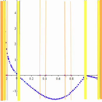
Figure 1: Imaginary part of coefficients $g_{3}^{3}$ (dots) on $\Sigma$, resonances of the third order (vertical lines), domain $\Sigma_{instable}$, where the imaginary parts of several coefficients $g_{i}^{j}$ do not vanish (yellow vertical lines) for $\gamma=9/7$.

Direct numerical computation from the system (8), (9), confirm our hypothesis on stability of equilibrium on $\Sigma_{stable}$.

Of course, our results concern stability with respect to small perturbations and the basin of attraction can be very small. The initial data that fall into the basin of attraction of a stable equilibrium can be found only numerically except of the case $b^{*}=0$ and $b^{*}=l$, where we obtained exact solution in Sec.5.1. However, even in this case the domain in the four-dimensional space of parameters $a_{0}=a(0),b_{0}=b(0),c_{0}=c(0),d_{0}=d(0)$ is very complicated. Indeed, as follows from (17), the trajectory will be periodic and therefore does not move away from the equilibrium for such initial data that $\det U(t)=1+l^{2}(C_{2}C_{4}-C_{1}C_{3})+(C_{2}+C_{4})l\sin lt+(C_{1}-C_{3})l\cos lt\neq 0$ for all $t>0$. Thus, the initial data corresponding to the basin of attraction have to satisfy the following condition:

$$-(a_{0}d_{0}+b_{0}c_{0})^{2}l^{2}+2\,(b_{0}+c_{0})(a^{2}_{0}d^{2}_{0}-b^{2}_{0}c^{2}_{0})l+((a_{0}-d_{0})^{2}-4b_{0}c_{0})(a_{0}d_{0}-b_{0}c_{0})^{2}<0.$$

In particular, this condition implies that increasing of $l$ at fixed parameters $a_{0},b_{0},c_{0},d_{0}$ stabilizes the motion.

The case $l=0$ ie exceptional. As follows from the results of Sec.4, in this case there is no nontrivial steady state solution an even the trivial equilibrium is unstable in the Lyapunov sense. Nevertheless, the oscillating regime can arise from elliptic perturbation of the axisymmetric state. Namely, as it was mentioned, in [2] it was shown that the system (10), an analog of (8), (9) for the case of the finite mass, is integrable for $\gamma=2$. This value of $\gamma$ corresponds to the shallow water equations. The formulae are very complicated and contain elliptic integrals, therefore it is hard to analyze them. Nevertheless, in [8], Ch.7, Sec.3 it is shown qualitatively that in this problem there exists oscillations and their period is estimated.

6 Comparison with numerics: localized vortex

We studied stability of the vortex corresponding to a very specific class of solutions. In fact, real vortices have the linear profile of velocity only near its center (see the discussion in [49]), therefore our results on the nonlinear stability or instability for the ”toy” solution (6), (7) not obliged to hold for ”realistic” solutions.

According [50], [51] the steady solution to (4), (5) can be constructed as follows. Let us consider arbitrary smooth enough stream function $\Phi=\Phi\left({x_{1}}^{2}+{x_{2}}^{2}\right)$. Then

$${\bf U}=\nabla_{\bot}\Phi=(\Phi_{x_{2}},-\Phi_{x_{1}})$$ (29)

and

$$\Pi=-\frac{1}{c_{0}}\,\left[2l\Phi+\int(\Phi_{x_{2}}\Phi_{x_{1}x_{2}}-\Phi_{x_{1}}\Phi_{x_{2}x_{2}})\,dx_{1}+\int(-\Phi_{x_{2}}\Phi_{x_{1}x_{1}}+\Phi_{x_{1}}\Phi_{x_{1}x_{2}})\,dx_{2}\right].$$ (30)

In [50] we choose the solution of such class with exponential decay for numerical computations in the context of big atmospherical vortices such as typhoons,i.e. this solution has the form

$$u_{1}^{0}\,=\,k\,B_{0}\,\sigma\,x_{2}\,e^{-\frac{\sigma}{2}\,\left({x_{1}}^{2}+{x_{2}}^{2}\right)},\qquad u_{2}^{0}\,=\,-B_{0}\,\sigma\,x_{1}\,e^{-\frac{\sigma}{2}\,\left({x_{1}}^{2}+{x_{2}}^{2}\right)},\quad k=1,$$ (31)

$$\Pi^{0}\,=\,-\,\frac{1}{2c_{0}}\,\left(\,B_{0}^{2}\,\sigma\,e^{-\sigma\,(x_{1}^{2}+x_{2}^{2})}\,-2\,l\,B_{0}\,e^{-\frac{\sigma}{2}\,(x_{1}^{2}+x_{2}^{2})}\right)+R_{0}.$$ (32)

is case corresponds to $\Phi=-B_{0}\,e^{-\frac{\sigma}{2}\,\left({x_{1}}^{2}+{x_{2}}^{2}\right)}$.

Nevertheless, based on experimental data, the meteorologists use a piecewise-continuous profile of tangential wind speed $V(r)$ such as $V(r)={\rm const}\cdot r$ for $r<R$ and $V(r)={\rm const}\cdot r^{-\frac{5}{8}}$ for $r>R$, where $R$ is the radius of the cyclone eye [60], so we study the numerical solution for initial conditions with ”natural” slower decay rate such as $x_{1}^{2}+x_{2}^{2}\to\infty$. To construct the steady solution, we use the following stream function

$$\Phi=\frac{B_{0}}{q}\left(1+\frac{\sigma}{2}\,\left({x_{1}}^{2}+{x_{2}}^{2}\right)\right)^{-q},\quad q>0,$$

which gives a family of initial data :

$$u_{1}^{0}\,=\,k\,B_{0}\,\sigma\,x_{2}\,\left(1+\frac{\sigma}{2}\,\left({x_{1}}^{2}+{x_{2}}^{2}\right)\right)^{-q-1},$$ (33)

$$u_{2}^{0}\,=\,-\,B_{0}\,\sigma\,x_{1}\,\left(1+\frac{\sigma}{2}\,\left({x_{1}}^{2}+{x_{2}}^{2}\right)\right)^{-q-1},$$

$$\Pi^{0}\,=\,-\,\frac{2}{c_{0}}\left[-\frac{B_{0}l}{q}\,\left(1+\frac{\sigma}{2}\,\left({x_{1}}^{2}+{x_{2}}^{2}\right)\right)^{-q}+\frac{B_{0}^{2}\sigma}{2q+1}\,\left(1+\frac{\sigma}{2}\,\left({x_{1}}^{2}+{x_{2}}^{2}\right)\right)^{-2q-1}\right]+R_{0},$$ (34)

They provide the steady solution for $k=1$.

It is easy to check that both velocities (31) and (33) have a linear profile with $b^{*}=B_{0}\sigma$ for those solutions close to the origin .

Easy computations show that for the both classes of data (31), (32) and (33), (34), the pressure has maximum or minimum at infinity for the same values of parameters as for the case of the velocity with linear profile. That is, (32) and (34) have a maximum at the origin provided $B_{0}\sigma/l=b^{*}/l\in(0,1)$. Nevertheless, if $B_{0}\sigma/l=b^{*}/l\in(1,s_{q})$, $s_{q}=\frac{2q+1}{q}>1,$ $q>0$, the value of $\Pi^{0}-R_{0}$ in (34) at zero is positive. This means that a small domain of low pressure exists on a background of high pressure. If $q\to\infty$, then $s_{q}\to 2$. The data with exponential decay (31), (32) correspond to a limit case, and the phenomenon takes place for $B_{0}\sigma/l=b^{*}/l\in(1,2)$. Thus, we can see that a stronger decay of initial data at infinity in some sense enlarges an ”anomalous low” domain.

Let us analyze whether the range of parameter $B_{0}\sigma$ that guarantees stability of the localized vortex like (31), (32) (or (33), (34)) can correspond to the respective range of stability of parameter $b^{*}$.

Basically, the answer is negative. Indeed, we have to compute the value of $G_{x_{1}}(0)$ (see Sec.3) with

$$\rho=\frac{\gamma}{c_{0}(\gamma-1)}(\Pi^{0}-R_{0})^{1/(\gamma-1)}$$

and estimate how far $G_{x_{1}}(0)$ is from the value of $A^{*}$ (see (13)). This requires the computation of improper integral with respect to $x_{1}$ and $x_{2}$. The integral can be taken analytically in the exponential case (32) with $\gamma=2$. It can be readily checked that here

$$G_{x_{1}}(0)=G_{x_{2}}(0)=-\frac{1}{2}\frac{\pi(B_{0}\sigma-8l)B_{0}}{\sigma^{2}c_{0}^{2}},\quad G_{x_{1}x_{2}}(0)=0,$$

$G_{x_{1}}(0)=G_{x_{2}}(0)=A^{*}$ for $B_{0}=0$ and $B_{0}=l\frac{c_{0}\sigma^{3}+8\pi}{c_{0}\sigma^{3}+\pi}.$ Thus, for sufficiently small values of $B_{0}$, the values of $A^{*}$ and $G_{x_{1}}(0)$ are close for any $\sigma$ and $c_{0}$. For large $B_{0}$ $A^{*}$ and $G_{x_{1}}(0)$, their values are close only for some specific parameters. This analysis is approximate, since in the velocity profile is not linear for the localized vortex, considered in this section, nevertheless, it helps us to understand the phenomenon.

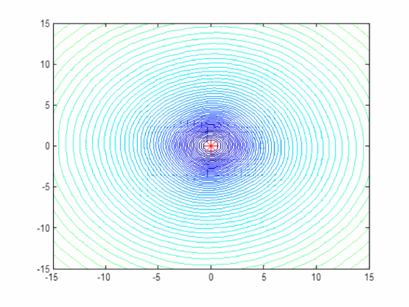
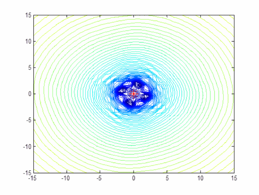
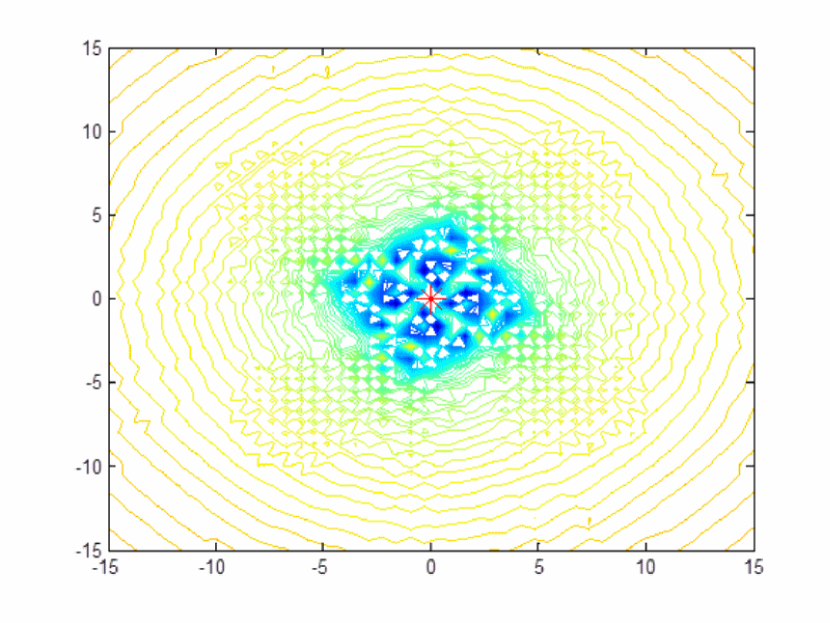
Figure 2: Transformation of vortex for cyclonic vorticity: $B_{0}=-10^{3}$, $B_{0}=-5\cdot 10^{3}$ and $B_{0}=-8\cdot 10^{3}$. $k=1.5$, $T\approx 24\rm h$, the horizontal scale is in kilometers

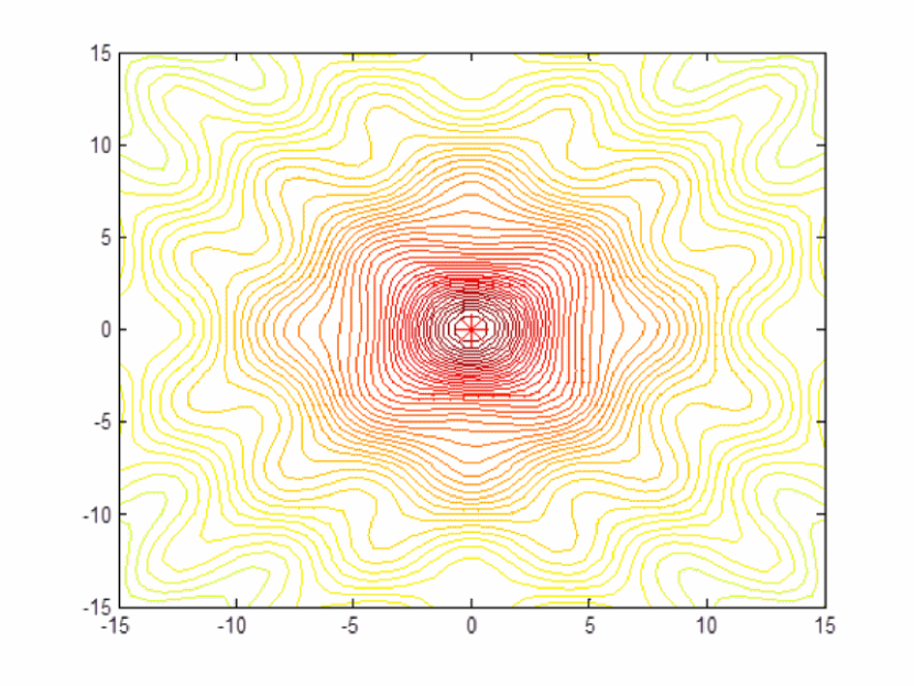
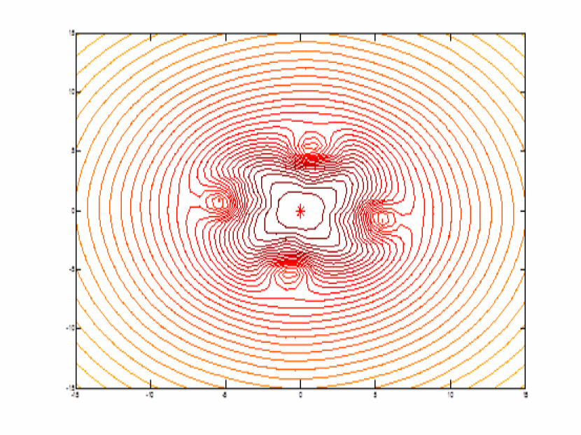
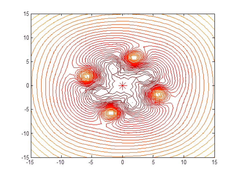
Figure 3: Transformation of vortex for anticyclonic vorticity: $B_{0}=10^{3}$, $B_{0}=7.5\cdot 10^{3}$ and $B_{0}=10^{4}$. $k=1.5$, $T\approx 24\rm h$, the horizontal scale is in kilometers

In the present paper, we studied numerically the deviation from the axial symmetry for stationary solution having exponential decay rate. Namely, we use initial data (31), (32), with $k\neq 1$, where parameter $k$ is a measure of deviation of velocity from the axial symmetry. Here, we take $k=1.5$ and $b^{*}=B_{0}\sigma.$

We used the same numerical method as in [50]. Namely, the computations were made by a modified Lax-Wendroff scheme, the method is second order accurate in both space and time variables [48], [36], [62]. The computations were performed on a $(400\times 400)$ uniform grid with the space step $\Delta x=\Delta y=0.64$ which corresponds to 12.8 km and the time step $\Delta t=0.0005$ which corresponds to 10 sec of the real time. We use the Neumann boundary condition set sufficiently far from the vortex domain. Nevertheless, it is possible to use more sophisticated non-reflecting boundary conditions (see [25]) and introduce an artificial viscosity to damp the oscillations [47].

The constants were chosen from the geophysical reasons, see [50]. Namely, the Coriolis parameter $l=7.3\times 10^{-5}\,{\rm s}^{-1},$ that corresponds to the latitude $30^{\circ}\,$ approximately, $c_{0}=0.1,\,R_{0}=10\,$(appropriate dimension), $\gamma=\frac{9}{7}$ (in the procedure of averaging over the height, the value of heat ratio for air changes), $\sigma=10^{-9}\rm m^{-2}$.

The results of computations show that the solution blows up if the value of $B_{0}\sigma$ does not belong to the segment $(b_{-},b_{+})$, $b_{-}\approx-1.31\cdot 10^{-5}$, $b_{+}\approx 1.85\cdot 10^{-5}$. We note that the left boundary $b_{-}$ is sufficiently close to the left boundary of stability domain for $b^{*}=l\frac{1-\sqrt{2}}{2}\approx 1.51\cdot 10^{-5}$. The right boundaries $b_{+}$ and $l\frac{1+\sqrt{2}}{2}$ are far from each other. Let us note that real values of vorticity in the atmosphere are sufficiently small. For example, in [50], we used $B_{0}\sigma=-10^{-6}\rm m^{2}/s.$

Figs.2 and 3 presents the level lines of pressure after one day for the initial data with exponential decay (31), (32).

Remark 5

We can see that the process of transition to breakdown is very similar to the case of formation of four vortices of a smaller size. Our graphs are similar to azimuthal Kelvin-Helmholtz instability, known from experimental works, e.g.[15].

Remark 6

The solution to the ODE system (8), (9) can blow up for certain initial data and the numerics confirms that this takes place in the instability domains. For the system (4), (5) the blow up means formation of infinite gradients of solution, e.g. the shock waves.

Remark 7

If we choose $\Phi$ as a smooth function with compact support, the initial data (29), (30) also have compact support. So, we can apply the stability theorem from [44], Sec.2.3.3, which says that the stationary solution of the initial boundary-value problem with the Dirichlet boundary condition is stable with respect to the class of smooth perturbations. Therefore, if for some range of parameters the perturbed solution is unstable, then it does not keep smoothness for all $t>0$.

7 Conclusion

We examine both theoretically and numerically the nonlinear stability of axisymmetric vortex in a compressible media. As in our previous works [49], [50], we consider two dimensional barotropic model obtained by averaging over the height of the primitive system of equations of the atmosphere dynamics. The resulting model is the 2D model of compressible barotropic rotating non-viscous medium. It can be used not only for studying the vortex process in atmosphere, but also in plasma, etc. In contrast to other models, where first the additional physically reasonable simplifications are made, we deal with special classes of solutions of the full system. This allows us to catch the complicated features of the full model.

We study how rotation of the coordinate frame and compressibility affect the stability of vortex. It is known that the axisymmetric form of vortex is stable with respect to asymmetric elliptical perturbations for the solutions of the incompressible Euler equations in a fixed coordinate frame (see [53] and references therein). Both linear analysis and computations show that a compressible vortex in a similar situation is basically instable [12]. We show that the situation is quite different for the compressible vortex in a rotating coordinate frame. Namely, the stability can take place only for a narrow range of parameters characterized by the rotation of vortex with respect to the Coriolis parameter. We prove that the motion is unstable if the parameter $b_{*}/l$, characterizing the relations between the vorticity and the Coriolis parameter, lies outside the segment $[(1-\sqrt{2})/2,(1+\sqrt{2})/2]$. Using the analytical-numerical method, we checked that the motion is unstable in a small neighborhood of boundary points $(1-\sqrt{2})/2$, $(1-\sqrt{2})/2$, as well as in a small neighborhood of the points $0$ and $1$, where the cyclonic motion changes to the anticyclonic one. For points of the segment $[(1-\sqrt{2})/2,(1+\sqrt{2})/2]$, up to the third order terms in the expansion of the normal form at the point of equilibrium, we checked numerically the sufficient condition of the stability.

In particular, the results imply that a rotation can stabilize the vortex. Similar results were obtained in [37], where the authors conclude that the rotation prevents blow up in a hydrodynamical model.

Furthermore, we study that the localized vortex with a linear profile of velocity near its center numerically. We conclude that for sufficiently small values of vorticity the range of parameters guaranteing stability approximately corresponds to the range of parameters guaranteing stability of the vortex with a linear profile. The reason for the phenomenon is explained analytically.

As it was mentioned, in [49], [50] we used the class of solutions with the properties of linear profile velocity to predict the trajectories of large geophysical vortices such as tropical cyclones. As it follows from [50], [51], the trajectory of localized vortex is not that far from the trajectory of vortex with a linear profile of velocity, if the divergence of velocity in this localized vortex is small in some sense. Thus, in the stable cases, we can compute the trajectory of vortices without much distortion even when the axial symmetry is breaking.

References

- [1] Aboelkassem Y and Vatistas G H 2007 New model for compressible vortices J. Fluids Eng 129 1073–1079
- [2] Anisimov S I and Lysikov Yu I 1970 Expansion of a gas cloud in vacuum Applied Meth.Mech.(PMM) 34 926-929
- [3] Anisimov S I and Inogamov N A 1974 Development of instability and loss of symmetry following isentropic compression of a spherical drop, JETP Lett.20 74-75
- [4] Ardalan K, Meiron D I and Pullin D I 1995 Steady compressible vortex flows: the hollow-core vortex array J. Fluid Mech.301 1- 17
- [5] Ball F K 1964 An exact theory of simple finite shallow water oscillations on a rotatirig earth 1st Australasian conference on hydraulics and fluid mechanics: proceedings (ed. R. Silvester). (MacMillan) 293 293–305
- [6] Bershader D 1995 Compressible Vortices in: Fluid Vortices Fluid Mechanics and Its Applications Vol 30 (Springer Netherlands) Ch.VII 291-316
- [7] Bibikov Yu N 1979 Local Theory of Nonlinear Analytic Ordinary Differential Equations (Lecture Notes in Mathematics, 702. Springer-Verlag: Berlin-New York) p 147
- [8] Bogoyavlensky O.I. 1985 Methods in the Qualitative Theory of Dynamical Systems in Astrophysics and Gas Dynamics (Springer Series in Soviet Mathematics Berlin-Heidelberg-New York: Springer-Verlag) p 301
- [9] Bruno A D 1989 Local methods in nonlinear differential equations (Springer Series in Soviet Mathematics. Springer-Verlag: Berlin)
- [10] Bruno A D 1971, 1972 Analytic form of differential equations, I and II Proceedings on the Moscow Mathematical Society 25 119–262 26 199– 239
- [11] Borisov A V, Mamaev I S and Kilin A A 2008 Hamiltonian dynamics of liquid and gas self-gravitating ellipsoids Russian Journal of Nonlinear Dynamics 4 363 - 406 (in Russian)
- [12] Chan W M, Shariff T K and Pulliam T H 1993 Instabilities of two-dimensional inviscid compressible vortices J. Fluid Mech. 253 173-209
- [13] Caillo P 2009 Absolute and convective instabilities of an inviscid compressible mixing layer: Theory and applications Phys. Fluids 21 104101
- [14] Chiocchia G 1989 A hodograph approach to the rotational compressible flow of an ideal fluid Q. Appl. Math. 47 513–528
- [15] Chomaz J-M, Ortiz S, Gallaire F and Billant P 2010 Stability of quasi two-dimensional vortices in: Fronts, Waves and Vortices in Geophysical Flows, Jan-Bert Flór (Ed.): Lect. Notes Phys. 805 (Springer, Berlin Heidelberg ) Chapter2
- [16] Chree C 1887 Vortex rings in a compressible fluid Proceedings of the Edinburgh Mathematical Society 6 59 -68
- [17] Colonius T, Lele S. K and Moin P 1991 The free compressible viscous vortex J. Fluid Mech. 230 45–73
- [18] Coulombel J-F and Secchi P 2008 Nonlinear compressible vortex sheets in two space dimensionsAnn. Sci. Ec. Norm. Super. 41 85–139
- [19] Dolzhansky F V 2013 Fundamentals of Geophysical Hydrodynamics Encyclopaedia of Mathematical Sciences V.103 (Berlin Heidelberg:Springer-Verlag)
- [20] Dyson J F 1968 Dynamics of a spinning gas cloud J. Math. Mech. (Indiana Univ. Math. J.) 18 91-101
- [21] Flierl G R 1988 On the instability of geostrophic vortices J. Fluid Mech 197 349–388
- [22] Fung Y T 1985 On the stability of vortex motions in compressible stratified fluids Journal of Fluids Engineering 107 73-78
- [23] Gaffet B 2001 Spinning gas clouds: Liouville integrability Journal of Physics A: Mathematical and General 34 2097-2109
- [24] Gill A E 1982 Atmosphere – Ocean Dynamics ( Academic Press: Cambridge)
- [25] Givoli D and Neta B 2003 High-order nonreflecting boundary conditions for the dispersive shallow water equations J. Comput. Appl. Math. 158 49–60
- [26] van Heijst G J F 2010 Dynamics of Vortices in Rotating and Stratified Fluids in: Fronts, Waves and Vortices in Geophysical Flows, Jan-Bert Flór (Ed.): Lect. Notes Phys. 805 (Springer, Berlin Heidelberg ) Chapter 1
- [27] Hiejima T 2015 Stability of compressible stream-wise vortices Physics of Fluids 27 074107
- [28] Hellier C 2001 Cataclysmic Variable Stars: How and Why They Vary (Springer Praxis: Berlin, Heidelberg, New-York)
- [29] Hopfinger E J and van Heijst G J F 1993 Vortices in rotating fluids Annu. Rev. Fluid Mech. 25 241–289
- [30] Khorrami M R 1995 Stability of a compressible axisymmetric swirling jet AIAA Journal 33 650–658
- [31] Kloosterziel R C and van Heijst G J F 1991 An experimental study of unstable barotropic vortices in a rotating fluid J. Fluid Mech. 223 1–24
- [32] Kloosterziel R C and van Heijst G J F 1992 The evolution of stable barotropic vortices in a rotating free-surface fluid J. Fluid Mech. 239 607–629
- [33] Lamb H 1975 Hydrodynamics (6th ed.) (Cambridge: Cambridge University Press)
- [34] Landau L D and Lifshits E M 1987 Fluid mechanics. 2nd ed., Volume 6 of Course of Theoretical Physics ( Oxford etc.: Pergamon Press)
- [35] Leblanc S, Le Duc A and Le Penven L 2000 On the stability of vortices in an ideal gas, in: Vortex Structures and Dynamics A. Maurel, P. Petitjeans (Eds.) (Berlin Heidelberg:Springer) 205–220
- [36] Lin X and Ballmann J 1995 A numerical scheme for axisymmetric elastic waves in solids Wave Motion 21 115–126
- [37] Liu H and Tadmor E 2004 Rotation prevents finite-time breakdown Phys. D 188 262–276
- [38] Lu G and Lele S K 1999 Inviscid instability of compressible swirling mixing layers Phys. Fluids 11 450–461
- [39] Meleshko V V and Aref H 2007 A Bibliography of Vortex Dynamics, 1858 – 1956 Advances in Applied Mechanics 41 197–292
- [40] Menshov I and Nakamura Yoshiaki 2005 Instability of isolated compressible entropy-stratified vortices Physics of Fluids17 034102
- [41] Nayfeh A H 2000 Perturbation Methods (Wiley-Interscience: New York)
- [42] Obukhov A M 1949 On the geostrophical wind Izv.Acad.Nauk (Izvestiya of Academie of Science of URSS), Ser. Geography and Geophysics XIII 281–306
- [43] Ovsiannikov L V 1956 New solution of hydrodynamics equations Dokl. Akad. Nauk SSS 111 47-9 (in Russian)
- [44] Padula M 2011 Asymptotic Stability of Steady Compressible Fluids (Lecture Notes In Mathematics Springer: Berlin, Heidelberg)
- [45] Pedlosky J 1979 Geophysical fluid dynamics (NY:Springer-Verlag)
- [46] Reid W T 1946 A matrix differential equation of Riccati type American Journal of Mathematics 68 237–246
- [47] Reutskiy S and Tirozzi B 2007 Forecast of the trajectory of the center of typhoons and the Maslov decomposition Russian Journal of Mathematical Physics, 14 232–237
- [48] Roache P.J. 1976 Computational fluid dynamics (Hermosa Publishers: Albuquerque)
- [49] Rozanova O S, Yu J-L and Hu C-K 2010 Typhoon eye trajectory based on a mathematical model: Comparing with observational data. Nonlinear Analysis: Real World Applications 11 1847–1861
- [50] Rozanova O S, Yu J-L and Hu C-K 2012 On the position of vortex in a two-dimensional model of atmosphere Nonlinear Analysis: Real World Applications13 1941–1954
- [51] Rozanova O S 2015 Frozen and almost frozen structures in the compressible rotating fluid Bulletin of the Brazilian Mathematical Society, New Series, Proceedings of HYP2014 (to appear) arXiv:1507.00690
- [52] Rozanova O S 2004 Classes of smooth solutions to the multidimensional balance laws of gas dynamic type on the riemannian manifolds In: Trends in mathematical physics (Nova Science: New-York)
- [53] Schecter D A, Dubin D H E, Cass A C, Driscoll C F, Lansky I M and O’Neil T.M. 2000 Inviscid damping of asymmetries on a two-dimensional vortex Phys. Fluids 12 2397
- [54] Rusak Z and Lee J H 2004 On the stability of a compressible axisymmetric rotating flow in a pipe Journal of Fluid Mechanics 501 25–42
- [55] Schecter D A and Montgomery M T 2003 On the symmetrization rate of an intense geophysical vortex Dynamics of Atmospheres and Oceans 37 55–88
- [56] Sheets R C 1982 On the structure of hurricanes as revealed by research aircraft data In: Intense atmospheric vortices. Proceedings of the Joint Simposium (IUTAM/IUGC) held at Reading (United Kingdom) July 14-17, 1981, edited by L.Begtsson and J.Lighthill, (Berlin-Heidelberg-New York: Springer-Verlag) p 33–49
- [57] Sipp D, Lauga E and Jacquin L 1999 Vortices in rotating systems: Centrifugal, elliptic and hyperbolic type instabilities Physics of Fluids 11 3716–3728
- [58] Starzhinskii V M 1980 Applied Methods in the Theory of Nonlinear Oscillations (Mir: Moscow) p 263
- [59] Thacker W C 1981 Some exact solutions to the nonlinear shallow water wave equations Journal of Fluid Mechanics 107 499–508
- [60] Vanderman L W and Usaf M 1962 An improved NWP model for forecasting the paths of tropical cyclones Monthly Weather Review January 19–22.
- [61] Wesson J 2004 Tokamaks International series of monographs on physics 118 (Oxford: Clarendon Press, Oxford University Press)
- [62] Zhang Y and Tabarrok B 1999 Modifications to the Lax-Wendroff scheme for hyperbolic systems with source terms Internat.J.Numer. Methods Eng. 44 27–40
- [63] Zheng Y and Zhang T 1997 Exact spiral solutions of the two-dimensional Euler equations Discrete and Continuous Dynamical Systems - Series A 3 117–133
- [64] Zheng Y and Zhang T 1998 Axisymmetric Solutions of the Euler equations for polytropic gases, Arch. Rat. Mech. Anal. 142 253–279
- [65] Zheng Y 2001 Systems of Conservation Laws: Two-Dimensional Riemann Problems Progress in Nonlinear Differential Equations and Their Applications 38 (Birkhäuser: Basel)