Quantum spin ice on the breathing pyrochlore lattice

Abstract

The Coulombic quantum spin liquid in quantum spin ice is an exotic quantum phase of matter that emerges on the pyrochlore lattice and is currently actively searched for. Motivated by recent experiments on the Yb-based breathing pyrochlore material Ba₃Yb₂Zn₅O₁₁, we theoretically study the phase diagram and magnetic properties of the relevant spin model. The latter takes the form of a quantum spin ice Hamiltonian on a breathing pyrochlore lattice, and we analyze the stability of the quantum spin liquid phase in the absence of the inversion symmetry which the lattice breaks explicitly at lattice sites. Using a gauge mean-field approach, we show that the quantum spin liquid occupies a finite region in parameter space. Moreover, there exists a direct quantum phase transition between the quantum spin liquid phase and featureless paramagnets, even though none of theses phases break any symmetry. At nonzero temperature, we show that breathing pyrochlores provide a much broader finite temperature spin liquid regime than their regular counterparts. We discuss the implications of the results for current experiments and make predictions for future experiments on breathing pyrochlores.

I Introduction

Frustrated magnetic materials provide a fertile arena to look for novel quantum phenomena. Frustration often leads to a large classical ground state degeneracy and quantum fluctuations are accordingly enhanced in quantum spin systems Moessner (2001); Balents (2010). When strong quantum fluctuations are taken to the extreme, they suppress any conventional magnetic order and may drive systems into a completely disordered quantum mechanical state, namely, a quantum spin liquid (QSL) Lee (2008); Balents (2010). QSLs are exotic quantum phases of matter, with long-range quantum entanglement, and are characterized by emergent gauge fields and deconfined fractionalized excitations Lee (2008); Balents (2010); Wen (2007).

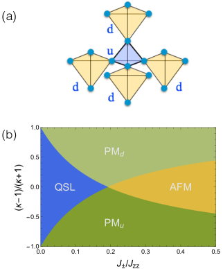
Figure 1: (Color online.) (a) The breathing pyrochlore lattice. The letter ‘u’ (‘d’) refers to the up- (down-) pointing tetrahedra. The bond lengths on up and down tetrahedra are different. (b) The phase diagram of the Hamiltonian $H$ in Eq. (1) at $T=0$. See the main text for a detailed discussion.

A three-dimensional $U(1)$ QSL with an emergent $U(1)$ gauge field and deconfined bosonic spinons has been proposed for rare-earth pyrochlore materials Hermele et al. (2004); Molavian et al. (2007); Ross et al. (2011); Savary and Balents (2012); Lee et al. (2012); Shannon et al. (2012a); Huang et al. (2014); Gingras and McClarty (2014); Kimura et al. (2013); Wan and Tchernyshyov (2012); Hao et al. (2014); Li and Chen (2016); Fritsch et al. (2013); Zhou et al. (2008); Chen (2016). In the context of rare-earth pyrochlores, Hamiltonians susceptible of hosting such QSLs are often referred to as “quantum spin ice” (QSI) Molavian et al. (2007); Ross et al. (2011); Savary and Balents (2012); Lee et al. (2012); Huang et al. (2014); Gingras and McClarty (2014), and their QSL is called QSI QSL or Coulombic QSL. Despite intense theoretical and experimental efforts, no definitive experimental evidence of such a QSL in QSI has been identified yet. This is partly because the underlying spin moment comes from 4f electrons whose exchange energy scale is usually very small. Thus, very challenging low temperature experiments are required to observe the intrinsic quantum properties of these materials, such as spinon deconfinement and the emergent gapless gauge photon. This raises an important question: Can we find an alternative physical system that realizes the QSI QSL ground state at a higher energy scale? A proposal has suggested to replace the spin degrees of freedom by charge degrees of freedom. The resulting cluster Mott insulator on the pyrochlore lattice can realize QSI physics in the charge sector at a much higher temperature scale Chen et al. (2014). Recently, a new material, Ba₃Yb₂Zn₅O₁₁, where the Yb atoms form a breathing pyrochlore lattice (see Fig. 1a), was synthesized. In contrast to the regular pyrochlore lattice, the breathing pyrochlore lattice has its up-pointing and down-pointing tetrahedra expanded and contracted, respectively, and thus breaks the lattice inversion symmetry at each lattice site Okamoto et al. (2013); Rau et al. (2016); Tanaka et al. (2014); Haku et al. (2016); Canals and Lacroix (1998, 2000); Tsunetsugu (2001); Li et al. (2016). Despite the a priori dominant antiferromagnetic interactions with a Curie-Weiss temperature $\Theta_{\text{CW}}=-6.7$K, the Yb local moments in Ba₃Yb₂Zn₅O₁₁ remain disordered down to $0.38$K Kimura et al. (2014). Motivated by the latter experiments, in this paper we propose that breathing pyrochlore materials are a new place to search for QSI physics, and in particular its QSL. Moreover, we argue that, due to the unique structure of breathing pyrochlores, the transition or crossover temperature from QSI to the higher-temperature thermal spin liquid phase occurs in breathing pyrochlores at a much higher temperature than in their ‘regular’ counterparts.

The breathing pyrochlore lattice harbors the same symmetries as the regular pyrochlore lattice except that it lacks the inversion symmetry centered at lattice sites. The spin model that we propose takes care of the absence of inversion symmetry by allowing different exchange couplings on the up and down tetrahedra. Near the symmetric limit, the system and the model are understood from the known results on the regular pyrochlores. There exists a QSI U(1) QSL phase in this limit. To understand the robustness of the QSL phase, we extend the gauge mean-field approach to access the parameter regime for the breathing pyrochlore system. As one observes in Fig. 1b, the QSL phase covers a large parameter regime. In addition, two paramagnetic (PM) phases are present in the asymmetric regime. These PM states are well understood in the strong asymmetric regime where the system breaks into decoupled tetrahedra. Since the ground state of the decoupled tetrahedron for our spin model is a singlet state, the PM in the asymmetric regime is smoothly connected to the simple product state of these decoupled tetrahedral singlets.

In the QSI $U(1)$ QSL phase, there are gapless gauge photon modes and deconfined and fractionalized spinon excitations. These exotic excitations are absent in the PM phases. In the gauge mean-field theory framework, the quantum phase transition from the QSL phase to the nearby PM phases is understood as the condensation of the spinons. The gauge photon picks up a mass due to the spinon condensation. This is essentially the Anderson-Higgs’ phenomenon, but it occurs in a system where the gauge field is emergent.

We further explore the finite temperature properties of the QSL phase. Both the perturbative argument and the gauge mean-field theory show that the onset temperature of the finite temperature QSL regime can be much higher than the regular pyrochlore system. This is because the asymmetric exchange couplings on the breathing pyrochlores allow the spins to fluctuate more effectively and thus enhance the energy scale of the collective spin fluctuations. The gauge mean-field theory is used to obtain the finite temperature phase diagram of the spin model. The persistence of the QSL physics to the high temperature regime gives a large room for the experimental confirmation.

The remaining parts of the paper are organized as follows. In Sec. II, we propose a minimal spin model for the breathing pyrochlore systems. In Sec. III, we implement the gauge mean-field mapping and obtain the full phase diagram of the spin model. We explain all the four phases and elucidate the nature of the phase transitions between them. In Sec. IV, we extend the gauge mean-field theory to finite temperatures and explore the properties of the system in the finite temperature regime. Finally, in Sec. V, we discuss the experimental consequences of the different phases. In the appendices, we provide the details of the derivation and the theoretical framework.

II Minimal model for breathing pyrochlores

In Ba₃Yb₂Zn₅O₁₁, the 4f electrons of a Yb³⁺ ion form a $J=7/2$ local moment due to the strong spin-orbit coupling of 4f electrons. The crystalline electric fields further split the eight-fold degeneracy of the $J=7/2$ manifold and lead to an on-site ground state with two-fold Kramers degeneracy. This local ground state doublet is separated from the excited doublets by a large crystal field energy gap of $\approx 500$K Kimura et al. (2014). Since the Curie-Weiss temperature $\Theta_{\text{CW}}=-6.7$K is much smaller than the crystal field energy gap, one then introduces a pseudospin-1/2 operator, $\bm{\tau}$, that operates within the local ground state doublet, to describe the low temperature magnetic properties of Ba₃Yb₂Zn₅O₁₁. Moreover, the strong crystal fields and spin-orbit coupling lead to a very large on-site anisotropy, which naturally singles out the local three-fold axis of the $D_{3d}$ point group, which corresponds to a $\langle 111\rangle$ crystallographic direction. Like the regular pyrochlore lattice, the local $\langle 111\rangle$ direction at a site is the direction that points into or out of the centers of the neighboring tetrahedra. We define the $z$ components of the pseudospins to be along their local $\langle 111\rangle$ axis (see Appendix. A).

We consider a minimal model for the pseudospins $\tau=1/2$ with Hamiltonian

$$H = \sum_{\langle ij\rangle\in\text{u}}{J_{zz}{\tau}^{z}_{i}\tau^{z}_{j}-J_{\pm}(\tau^{+}_{i}\tau^{-}_{j}+\tau^{-}_{i}\tau^{+}_{j})}$$ (1)

$$+ \sum_{\langle ij\rangle\in\text{d}}\kappa{\big{[}J_{zz}{\tau}^{z}_{i}\tau^{z}_{j}-J_{\pm}(\tau^{+}_{i}\tau^{-}_{j}+\tau^{-}_{i}\tau^{+}_{j})\big{]}},$$

where ${\tau^{\pm}_{i}=\tau^{x}_{i}\pm i\tau^{y}_{i}}$. The hallmark of breathing pyrochlore systems is the absence of inversion symmetry centered at lattice sites, and the parameter $\kappa$ captures this property. More precisely, it parametrizes the asymmetry of the spin interactions between the up-pointing (labelled by ‘u’) and down-pointing (labelled by ‘d’) tetrahedra of the breathing pyrochlore lattice. On a regular pyrochlore lattice, due to the presence of inversion symmetry, one has $\kappa=1$. In breathing pyrochlore systems, the asymmetry parameter $\kappa$ should generically deviate from 1.

Even though the Hamiltonian $H$ is not the most general spin model obtained from a full space group symmetry analysis of the breathing pyrochlore lattice Ross et al. (2011); Savary and Balents (2012), the Hamiltonian $H$ is sufficient for the purpose of understanding the stability of the QSI QSL phase against the breathing distortion, as well as some additional features of breathing pyrochlore systems. Due to the strong spin-orbit coupling of the Yb 4f electrons, the interactions between local moments should be both bond dependent and anisotropic in (effective) spin space Witczak-Krempa et al. (2014); Chen et al. (2010); Chen and Balents (2011), which thus introduces additional complications. Its study will be discussed in future work.

The Hamiltonian $H$ has been studied both theoretically and numerically on the regular pyrochlore lattice, where $\kappa=1$ Hermele et al. (2004); Banerjee et al. (2008); Savary and Balents (2012); Lv et al. (2015). There, in the Ising limit with $J_{\pm}=0$, the system favors the extensively-degenerate “2-in 2-out” spin ice ground state manifold. A small and finite transverse coupling $J_{\pm}$ generates a six-spin ring exchange around the hexagonal plaquettes of the pyrochlore lattice and allows the system to fluctuate quantum mechanically within the ice manifold Hermele et al. (2004); Savary and Balents (2012, 2016); Gingras and McClarty (2014); Lee et al. (2012); Huang et al. (2014); Hao et al. (2014). By mapping the effective ring exchange Hamiltonian in the perturbative regime ($J_{zz}\gg|J_{\pm}|$) onto a lattice gauge theory that operates within the spin ice manifold, it was argued that the system exhibits a $U(1)$ QSL phase, i.e. the QSI QSL state Hermele et al. (2004). This theoretical result was later confirmed numerically by quantum Monte Carlo calculations in the regime with $J_{\pm}>0$ Banerjee et al. (2008); Lv et al. (2015); Kato and Onoda (2015); Shannon et al. (2012b). In the breathing pyrochlore lattice, the perturbative argument in the limit $J_{zz}\gg|J_{\pm}|$ remains valid at least when the parameter $\kappa$ does not strongly deviate from 1 (see Appendix. B). Moreover, in general, the QSI QSL state is a robust quantum phase of matter and is stable against any small local perturbation Hermele et al. (2004). Both arguments confirm that the QSL state of QSI should be the ground state of the minimal model $H$ at least in the regime with $J_{zz}\gg|J_{\pm}|$ and $\kappa\approx 1$.

III Ground state phase diagram

To investigate the stability of the QSI QSL state further and to obtain its proximate phases on the breathing pyrochlore lattice, we apply the recently developed non-perturbative slave-particle construction Savary and Balents (2012); Lee et al. (2012). For this purpose, we first enlarge the physical Hilbert space to make the spinon and $U(1)$ gauge field variables explicit, and we express the effective spin operators as

$$\tau^{+}_{i} \equiv \tau^{+}_{{\bf r},{\bf r}+{\bf e}_{\mu}}=\Phi^{\dagger}_{\bf r}\Phi^{\phantom{\dagger}}_{{\bf r}+{\bf e}_{\mu}}\mathsf{s}^{+}_{{\bf r},{\bf r}+{\bf e}_{\mu}},$$ (2)

$$\tau^{z}_{i} \equiv \tau^{z}_{{\bf r},{\bf r}+{\bf e}_{\mu}}=\mathsf{s}^{z}_{{\bf r},{\bf r}+{\bf e}_{\mu}},$$ (3)

where ${\bf r}$ belongs to the u sublattice of the diamond lattice that is formed by the centers of the up-pointing tetrahedra in the breathing pyrochlore lattice (see Fig. 1), where the vectors ${\bf e}_{\mu}$ (with $\mu=1,2,3,4$) connect ${\bf r}$ with the centers of the neighboring tetrahedra, and $i$ is the breathing pyrochlore lattice site that is shared by the two tetrahedra that are centered at the positions ${\bf r}$ and ${{\bf r}+{\bf e}_{\mu}}$. $\Phi^{\dagger}_{\bf r}$ ($\Phi^{\phantom{\dagger}}_{\bf r}$) is the (bosonic) spinon creation (annihilation) operator at site ${\bf r}$, and $\mathsf{s}^{z}_{{\bf r}{\bf r}^{\prime}},\mathsf{s}^{\pm}_{{\bf r}{\bf r}^{\prime}}$ are “spin”-$1/2$ operators that act as $U(1)$ gauge fields. To preserve the physical spin Hilbert space, we further impose the constraint

$${Q}_{\bf r}=\eta_{\bf r}\sum_{\mu}\mathsf{s}^{z}_{{\bf r},{\bf r}+\eta_{\bf r}{\bf e}_{\mu}},$$ (4)

where $\eta_{\bf r}=\pm 1$ for ${\bf r}\in\text{u/d}$ sublattice. The operator ${Q}_{\bf r}$ counts the number of spinons and satisfies $[\phi_{\bf r},Q_{{\bf r}^{\prime}}]=i\delta_{{\bf r}{\bf r}^{\prime}}$, where $\phi_{\bf r}$ is a $2\pi$ periodic angular variable defined as $\Phi_{\bf r}\equiv e^{-i\phi_{\bf r}}$, with $\Phi^{\dagger}_{\bf r}\Phi^{\phantom{\dagger}}_{\bf r}=1$, by construction. In terms of these slave particle operators, the Hamiltonian $H$ is rewritten as

$$H = \sum_{{\bf r}\in\text{u}}\frac{J_{zz}}{2}Q_{\bf r}^{2}-\kappa J_{\pm}\sum_{{\bf r}\in\text{d},\mu\neq\nu}\Phi^{\dagger}_{{\bf r}-{\bf e}_{\mu}}\Phi^{\phantom{\dagger}}_{{\bf r}-{\bf e}_{\nu}}\mathsf{s}^{-}_{{\bf r},{\bf r}-{\bf e}_{\mu}}\mathsf{s}^{+}_{{\bf r},{\bf r}-{\bf e}_{\nu}}$$

$$+ \sum_{{\bf r}\in\text{d}}\frac{\kappa J_{zz}}{2}Q_{\bf r}^{2}-J_{\pm}\sum_{{\bf r}\in\text{u},\mu\neq\nu}\Phi^{\dagger}_{{\bf r}+{\bf e}_{\mu}}\Phi^{\phantom{\dagger}}_{{\bf r}+{\bf e}_{\nu}}\mathsf{s}^{-}_{{\bf r},{\bf r}+{\bf e}_{\mu}}\mathsf{s}^{+}_{{\bf r},{\bf r}+{\bf e}_{\nu}}.$$

The above Hamiltonian describes the bosonic spinons ($\Phi_{\bf r}$) hopping on the dual diamond lattice in the background of a fluctuating $U(1)$ gauge field ($\mathsf{s}^{\pm}_{{\bf r}{\bf r}^{\prime}}$). It is manifestly invariant under the local $U(1)$ gauge transformation $\Phi_{\bf r}\rightarrow\Phi_{\bf r}e^{-i\chi_{\bf r}},\mathsf{s}^{\pm}_{{\bf r}{\bf r}^{\prime}}\rightarrow\mathsf{s}^{\pm}_{{\bf r}{\bf r}^{\prime}}e^{\pm i(\chi_{{\bf r}^{\prime}}-\chi_{\bf r})}$.

We apply gauge mean field theory (gMFT) Savary and Balents (2012); Lee et al. (2012); Savary and Balents (2013) to analyze the phase diagram of $H$. To proceed, we first note that the (low-energy) ring exchange Hamiltonian that operates within the spin ice manifold favors a zero gauge flux for $J_{\pm}>0$ (see Appendix. B). Therefore, we choose a mean-field ansatz where the spinons experience a zero gauge flux through each hexagon of the pyrochlore lattice. We decouple Eq. (LABEL:eq4) into the spinon and gauge field sectors, and select a gauge such that the spinon hopping is uniform. With this gauge choice, the gMFT connects to and reproduces the results of the $J_{\pm}\ll J_{zz},|\kappa-1|\ll 1$ limit where the solution is known from perturbation theory and numerical calculations Hermele et al. (2004); Savary and Balents (2012, 2016); Gingras and McClarty (2014); Lee et al. (2012); Huang et al. (2014); Hao et al. (2014); Banerjee et al. (2008); Lv et al. (2015); Kato and Onoda (2015); Shannon et al. (2012b). The gMFT phase diagram is depicted in Fig. 1b. The QSL covers a wide range of $\kappa$ in parameter space. When the spinons on the u and d sublattices of the diamond lattice are both gapped (and thus do not condense), the system is in the QSI QSL phase (see Table 1) and the low energy properties, such as algebraic correlations, are controlled by the gapless $U(1)$ gauge photon.

Phase	$\langle\Phi_{\bf r}\rangle,{\bf r}\in\text{u}$	$\langle\Phi_{\bf r}\rangle,\bf r\in\text{d}$	$\langle\mathsf{s}^{\pm}\rangle$	$\langle\mathsf{s}^{z}\rangle$	$|\langle\vec{\mathsf{s}}\rangle|$
QSL	$=0$	$=0$	$\neq 0$	$=0$	$\neq 0$
AFM	$\neq 0$	$\neq 0$	$\neq 0$	$=0$	$\neq 0$
PM${}_{\text{u}}$	$\neq 0$	$=0$	$\neq 0$	$=0$	$\neq 0$
PM${}_{\text{d}}$	$=0$	$\neq 0$	$\neq 0$	$=0$	$\neq 0$
TSL	$=0$	$=0$	$=0$	$=0$	$=0$

Table 1: Different ground state phases with their order parameters in gMFT. QSL and TSL stand for the quantum spin ice quantum spin liquid, and thermal spin liquid, respectively.

We treat the QSI QSL as the parent state and analyze the proximate phases obtained via an Anderson-Higgs transition. We first consider leaving the QSL by condensing one spinon flavor (i.e. condensing the spinons on one diamond sublattice) while keeping the other spinon flavor uncondensed. This is certainly reasonable due to the absence of on-site inversion symmetry in the breathing pyrochlore lattice. For concreteness, we condense the spinons on the down sublattice with $\langle\Phi_{\bf r}\rangle\neq 0$ for ${\bf r}\in$ d sublattice. As a consequence, the $U(1)$ gauge field picks up a mass through the usual Anderson-Higgs mechanism. What is surprising is that the resulting state is not magnetically ordered. This is because the spinons on the u sublattice are not condensed. According to the slave particle construction in Eq. (2), this proximate state of the QSI QSL, obtained by condensing spinons on one sublattice but not on the other, does not develop any transverse magnetic long range order following

$$\langle\tau^{\pm}_{{\bf r}{\bf r}^{\prime}}\rangle=\langle\Phi_{\bf r}^{\dagger}\rangle\langle\Phi_{{\bf r}^{\prime}}^{\phantom{\dagger}}\rangle\langle\mathsf{s}^{\pm}_{{\bf r}{\bf r}^{\prime}}\rangle=0.$$ (6)

This paramagnetic state preserves time reversal symmetry and all the lattice symmetries of the breathing pyrochlore lattice. We thus dub this paramagnetic (PM) state PM${}_{\text{u}}$ in Fig. 1b and Table 1.

To understand the nature of the PM_u/d phases better, especially outside of gMFT, we consider the limiting case $\kappa\rightarrow 0$. In this special limit, the breathing pyrochlore system reduces to a set of decoupled up-pointing tetrahedra, i.e. set of four spins. Since a tetrahedron contains a finite number of spins (it is a finite system), its ground state must preserve all the symmetries of the system. For each up-pointing tetrahedron, the local magnetization $\sum_{i\in\text{u}}\tau^{z}_{i}$ commutes with the Hamiltonian and is therefore a good quantum number, and the ground state is unique with $\sum_{i\in\text{u}}\tau^{z}_{i}=0$. Since the tetrahedra are decoupled, the many-body ground state is simply a product state of the single-up-tetrahedron ground states. Hence, the system is an obvious paramagnetic state, preserving all symmetries. A finite and small $\kappa$ introduces inter-up-tetrahedral couplings but does not significantly alter the ground state. Moreover, due to the weak $\tau^{z}$ coupling on the down-pointing tetrahedra, the local magnetization ($\sum_{i\in\text{d}}\tau^{z}_{i}$) on each down-pointing tetrahedron is strongly fluctuating quantum mechanically and thus is not a good quantum number. These features are exactly reproduced by the gMFT description of the PM_u: the spinon condensate on the down tetrahedra corresponds to an ill-defined spinon number $Q_{\mathbf{r}\in{\rm d}}=\sum_{i\in\text{d}}\tau^{z}_{i}$, and the single-tetrahedron ground state with its (small) ‘cat’ state on the up tetrahedra preserves all symmetries and corresponds to $\langle\Phi_{\mathbf{r}\in{\rm u}}\rangle=0$. Therefore, the gMFT approach provides a good description of the $\kappa\rightarrow 0$ limit, like it did for the QSI QSL phase.

The state obtained by instead condensing the spinons on the down sublattice, is naturally labelled PM${}_{\text{d}}$. Like the relation between the PM${}_{\text{u}}$ and the $\kappa\rightarrow 0$ limit, the PM${}_{\text{d}}$ is smoothly connected to the paramagnetic state in the limit $\kappa\rightarrow\infty$, and the gMFT also provides a good description of this limit. As the PM${}_{\text{u}}$ and the PM${}_{\text{d}}$ have neither gapless emergent gauge photon nor spontaneous continuous symmetry breaking, the system is fully gapped in these two phases. The quantum phase transition from the gapless QSI QSL to the gapped PM${}_{\text{u}}$ or PM${}_{\text{d}}$ is described by the condensation of one critical bosonic spinon mode coupled to a fluctuating $U(1)$ gauge field. This quantum phase transition is not present for the regular pyrochlores and is a new feature of the breathing pyrochlores.

A condensate of both spinon flavors is obtained for example by increasing $J_{\pm}/J_{zz}$ and keeping a moderate $\kappa$. The resulting state breaks time reversal symmetry and develops magnetic order via

$$\langle\tau^{\pm}_{{\bf r}{\bf r}^{\prime}}\rangle=\langle\Phi_{\bf r}^{\dagger}\rangle\langle\Phi_{{\bf r}^{\prime}}^{\phantom{\dagger}}\rangle\langle\mathsf{s}^{\pm}_{{\bf r}{\bf r}^{\prime}}\rangle\neq 0.$$ (7)

In terms of the original physical magnetic moments, this ordered state is an AFM state and the magnetic unit cell is identical to that of the crystal. Moreover, the direct treatment of the limiting case with a dominant $J_{\pm}/J_{zz}$ and a moderate $\kappa$ also leads to a transverse spin ordering, which is again consistent with the results from the gMFT approach.

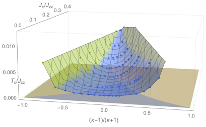
Figure 2: (Color online.) Phase diagram in the $\kappa$-$J_{\pm}/J_{zz}$-$T/J_{zz}$ space. The three-dimensional surface indicates the first-order transition between the phases akin to the zero-temperature phases, namely the QSL, AFM, PM_u,d (below the surface), and the TSL (above the surface). The colors on the surface correspond to those of the phases immediately below the surface.

IV Nonzero temperature spin liquid regime of QSI

Now we turn to the nonzero temperature behavior of the system. Strictly speaking, the QSI QSL is truly a quantum phase and cannot exist at non-zero temperatures. This is because the topological defects (or magnetic monopole excitations) of the emergent $U(1)$ gauge field Hermele et al. (2004) in the QSI QSL state are point-like particles and have a finite energy Savary and Balents (2013). These topological excitations can always be created with a finite concentration at a non-zero temperature so that the infinitesimal temperature phase above the QSL can be smoothly connected to the high-temperature phase Savary and Balents (2013). The above general argument does not however preclude the existence of a non-generic first-order transition, which indeed is found in nonzero temperature gMFT between the low temperature regime akin to the QSL, and a classical regime where the entropy is released and the spinons lose coherence: the thermal spin liquid (TSL) regime. This TSL regime is the one found in classical spin ices Bramwell and Gingras (2011); den Hertog and Gingras (2000); Gardner et al. (2010). Regardless of whether a crossover or a first order transition occurs between the low temperature spin liquid regime and a thermal spin ice regime, the temperature scale of either is set by the strength of the ring exchange Hermele et al. (2004); Savary and Balents (2013), $J_{\text{ring}}=6(\kappa^{3}+\kappa^{-2})J_{\pm}^{3}/J_{zz}^{2}$. The minimum of $(\kappa^{3}+\kappa^{-2})$, and hence that of $J_{\text{ring}}$, occurs at $\kappa\approx 0.92$ (see Appendix. B). We therefore expect that, at any given value of $J_{\pm}/J_{zz}$, the crossover/transition temperature is usually enhanced for the breathing pyrochlore lattice as compared to that in its regular counterpart. This suggests that the QSL physics can be observed at higher temperatures in breathing pyrochlore systems.

To explicitly confirm the above observation, we carry out a nonzero temperature gMFT calculation for the minimal model Eq. (1). The calculation is carried out variationally, and the details are given in Appendix. D. The gMFT finds a direct first-order transition, with the transition temperature shown on the surface plotted on Fig. 2. Just as we expect, the transition temperature is significantly enhanced as $\kappa$ deviates from 1. This transition can be regarded as a “thermal confinement” transition as discussed in early literature Kamiya et al. (2015); Kato and Onoda (2015); Savary and Balents (2013).

Like many other mean field treatments, the gMFT neglects the gauge field fluctuations and thus overestimates the transition temperature. This can be seen for example through the analytical gMFT expression (see Appendix. D) obtained in the limit of very low temperature, $\kappa\approx 1$ and small $J_{\pm}/J_{zz}$:

$$k_{B}T_{c}^{\rm gMFT}=\frac{3J_{\pm}^{2}}{32J_{zz}\ln 2}\left(\kappa^{2}+\frac{1}{\kappa}\right)$$ (8)

(to be compared, in that limit, with the $J_{\rm ring}$ scale of perturbation theory). Nevertheless, the gMFT does qualitatively capture the thermal activation of the gapped spinon excitations which effectively reduces the magnetic stiffness and thus destabilizes the QSL.

V Discussion

Since the featureless PM phases (PM${}_{\text{u}}$ or PM${}_{\text{d}}$) are also connected to the high-temperature paramagnet and do not have any ordering, one may then wonder how to distinguish the QSI QSL state and the featureless PM phases of Fig. 1b in experiment. QSL has a linearly-dispersing gauge photon mode that gives rise to a low-temperature heat capacity $C_{v}\sim T^{3}$ whose prefactor can be quite large in 4f electron systems Savary and Balents (2012); Shannon et al. (2012a); Huang et al. (2014). Inelastic neutron scattering and/or NMR spin lattice relaxation time measurements are direct probes of the gapless gauge photon. In contrast, since the PM${}_{\text{u,d}}$ is fully gapped, the heat capacity should have an activated temperature dependence.

Thermodynamic measurements on the breathing pyrochlore material Ba₃Yb₂Zn₅O₁₁ have not found any indication of ordering down to 0.38K Kimura et al. (2014). The magnetic entropy density extracted from the heat capacity data above 0.38K is close to $0.75{\text{R}}\ln(2)$ per site, and the missing entropy ($0.25{\text{R}}\ln(2)$ per site) was interpreted in terms of an AFM Heisenberg model, effectively acting only within the smaller tetrahedra at the accessible temperatures Kimura et al. (2014): this model of decoupled tetrahedra has a two-fold (the two singlet states of four coupled $S=1/2$) degeneracy per small tetrahedron, giving, per site, an entropy of $0.25{\text{R}}\ln(2)$. In this picture, the exchange coupling on the large tetrahedra then operates perturbatively on the singlet manifold and lifts the degeneracy only at a much lower energy scale. (The Heisenberg model for arbitrary small to large exchange was also recently studied classically in detail in Ref. Benton and Shannon, 2015.) Here we provide an alternative explanation for the experimental value of the low-temperature magnetic entropy density.

First, we argue that, due to strong spin-orbit coupling, the $J=7/2$ local moment of the Yb³⁺ ion is an entangled state of the $L=3$ orbital angular momentum and $S=1/2$ spin moment, and an isotropic model, such as the Heisenberg model, is therefore unlikely Witczak-Krempa et al. (2014); Chen and Balents (2008); Chen et al. (2010); *PhysRevB.84.094420. This is especially true considering that the main contribution to the local doublet comes from the orbital degree of freedom Ross et al. (2011), which naturally singles out the local $z$ directions. This non-Heisenberg exchange, and more specifically its $D_{3d}$ anisotropy, points to the Pauling entropy of thermal spin ice in the temperature regime $J_{\text{ring}}\lesssim T\lesssim\min(1,\kappa)J_{zz}$ Savary and Balents (2013). Indeed, current experiments cannot rule out this possibility as Pauling’s entropy ($0.5{\text{R}}\ln(3/2)\approx 0.20{\text{R}}$ per site) is very close to the reported $0.25{\text{R}}\ln(2)\approx 0.17{\text{R}}$ per site, with these two values likely being within error bars of one another.

At this point, neutron scattering experiments are crucially needed to check whether the system might be in the ice manifold and whether quantum spin ice QSL physics appears below $0.38$K. It will also be interesting to look for QSL physics in other breathing pyrochlore systems with other rare earth elements Rabbow and Müller-Buschbaum (1996). Indeed, in general, based on our theoretical results, breathing pyrochlores appear as a promising playground for the discovery of quantum spin ice physics and novel quantum phase transitions, and certainly warrant further investigation.

VI Acknowledgements

LS acknowledges Leon Balents for previous collaborations on related work. LS is supported by a postdoctoral fellowship from the Gordon and Betty Moore foundation, EPiQS initiative, Grant No. GBMF4303. HYK and YBK are supported by NSERC, Centre for Quantum Materials at UofT. GC would like to thank the hospitality of Fuchun Zhang and Yi Zhou for supporting his stay at Zhejiang University (Hangzhou, People’s Republic of China) in April and May 2015 when and where part of the work was carried out. GC is supported by the Starting-up fund of Fudan University (Shanghai, People’s Republic of China) and Thousand-Youth-Talent Program of People’s Republic of China. Notes added: we recently noticed an interesting work on a related topic Rau et al. (2016). The view of Ref. Rau et al., 2016 is complementary to ours.

Appendix A Local coordinate system

The Bravais lattice of the breathing pyrochlore lattice is a FCC lattice. We choose the basis vectors to be

$${\bf a}_{1}=\frac{1}{2}[011],\;{\bf a}_{2}=\frac{1}{2}[101],\;{\bf a}_{3}=\frac{1}{2}[110],$$ (9)

where the lattice constant is set to be unity. We define the reference points of the four sublattices as

$${\bf b}_{1} = [000],$$ (10)

$${\bf b}_{2} = c[011],$$ (11)

$${\bf b}_{3} = c[101],$$ (12)

$${\bf b}_{4} = c[110],$$ (13)

where $c=1/4$ for the regular pyrochlore lattice and $c\neq 1/4$ for the breathing pyrochlore lattice. The local coordinate system at each sublattice is then defined in Table 2.

$\mu$	1	2	3	4
$\hat{x}_{\mu}$	$\frac{1}{\sqrt{2}}[\bar{1}10]$	$\frac{1}{\sqrt{2}}[\bar{1}\bar{1}0]$	$\frac{1}{\sqrt{2}}[110]$	$\frac{1}{\sqrt{2}}[1\bar{1}0]$
$\hat{y}_{\mu}$	$\frac{1}{\sqrt{6}}[\bar{1}\bar{1}2]$	$\frac{1}{\sqrt{6}}[\bar{1}1\bar{2}]$	$\frac{1}{\sqrt{6}}[1\bar{1}\bar{2}]$	$\frac{1}{\sqrt{6}}[112]$
$\hat{z}_{\mu}$	$\frac{1}{\sqrt{3}}[111]$	$\frac{1}{\sqrt{3}}[1\bar{1}\bar{1}]$	$\frac{1}{\sqrt{3}}[\bar{1}1\bar{1}]$	$\frac{1}{\sqrt{3}}[\bar{1}\bar{1}1]$

Table 2: The local coordinate systems for the four sublattices of the breathing pyrochlore lattice.

Appendix B Ring exchange

In the perturbative regime or in the Ising limit, one can treat the $J_{\pm}$ and $\kappa J_{\pm}$ terms as a perturbation. We thus write the Hamiltonian $H$ as

$$H=H_{\text{Ising}}+H^{\prime},$$ (14)

where $H_{\text{Ising}}$ and $H^{\prime}$ are the unperturbed part and the perturbation part, respectively. We have

$$H_{\text{ring}} = \sum_{\langle ij\rangle\in\text{u}}J_{zz}\tau_{i}^{z}\tau_{j}^{z}+\sum_{\langle ij\rangle\in\text{d}}\kappa J_{zz}\tau_{i}^{z}\tau_{j}^{z}$$ (15)

$$H^{\prime} = -\sum_{\langle ij\rangle\in\text{u}}{J_{\pm}}(\tau_{i}^{+}\tau_{j}^{-}+h.c.)$$ (16)

$$-\sum_{\langle ij\rangle\in\text{d}}{\kappa J_{\pm}}(\tau_{i}^{+}\tau_{j}^{-}+h.c.).$$

The Ising exchange $H_{\text{Ising}}$ favors a highly degenerate spin ice ground state. The perturbation $H^{\prime}$ acts on the ice manifold. Treating $H^{\prime}$ in the 3rd order degenerate perturbation theory, we obtain a ring exchange effective Hamiltonian Hermele et al. (2004),

$$H_{\text{eff}}=-\sum_{\hexagon}J_{\text{ring}}(\tau_{1}^{+}\tau_{2}^{-}\tau_{3}^{+}\tau_{4}^{-}\tau_{5}^{+}\tau_{6}^{-}+h.c.),$$ (17)

where 1,2,3,4,5,6 label the 6 pseudospins on the perimeter of an elementary hexagon on the breathing pyrochlore lattice and

$$J_{\text{ring}}=6(\kappa^{3}+\kappa^{-2})\frac{J_{\pm}^{3}}{{J_{zz}^{2}}}.$$ (18)

We map the effective Hamiltonian $H_{\text{eff}}$ to a $U(1)$ lattice gauge theory by expressing $\tau^{z}_{i}=E_{{\bf r}{\bf r}^{\prime}},\tau^{\pm}_{i}=e^{\pm iA_{{\bf r}{\bf r}^{\prime}}}$, where ${\bf r}$ (${\bf r}^{\prime}$) belongs to the u (d) sublattice of the diamond lattice formed by the centers of the tetrahedra and $i$ is the pyrochlore lattice site shared by the two neighbor tetrahedra at ${\bf r}$ and ${\bf r}^{\prime}$ (see Fig. 1a). $E$ and $A$ are the lattice electric field and the vector gauge potential defined on the diamond lattice and $E_{{\bf r}{\bf r}^{\prime}}=-E_{{\bf r}^{\prime}{\bf r}},A_{{\bf r}{\bf r}^{\prime}}=-A_{{\bf r}^{\prime}{\bf r}}$ Hermele et al. (2004). In terms of the gauge field operators, the low energy ring exchange is recast as the following $U(1)$ gauge theory on the diamond lattice,

$$H_{\text{eff}}=-K\sum_{\varhexagon}\cos(\nabla\times A)_{\varhexagon}$$ (19)

where $\varhexagon$ refers to the elementary hexagons on the diamond lattice and the magnetic stiffness $K=2J_{\text{ring}}$ is plotted in Fig. 3 as a function of $\kappa$.

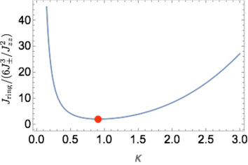
Figure 3: (Color online.) The ring exchange as a function of $\kappa$. The (red) dot is the position of the minimum and is at $\kappa\approx 0.92$.

Appendix C Gauge mean field theory for the ground state

In the gauge mean field theory, we decouple the Hamiltonian $H$ into the spinon and gauge sectors. The spinon sector mean field Hamiltonian is written as

$$H_{\text{u}} = \sum_{{\bf r}\in\text{u}}\frac{J_{zz}}{2}Q_{\bf r}^{2}-\kappa J_{\pm}\langle\mathsf{s}^{\pm}\rangle^{2}\sum_{{\bf r}\in\text{d},\mu\neq\nu}\Phi^{\dagger}_{{\bf r}-{\bf e}_{\mu}}\Phi^{\phantom{\dagger}}_{{\bf r}-{\bf e}_{\nu}},$$ (20)

$$H_{\text{d}} = \sum_{{\bf r}\in\text{d}}\frac{\kappa J_{zz}}{2}Q_{\bf r}^{2}-J_{\pm}\langle\mathsf{s}^{\pm}\rangle^{2}\sum_{{\bf r}\in\text{u},\mu\neq\nu}\Phi^{\dagger}_{{\bf r}+{\bf e}_{\mu}}\Phi^{\phantom{\dagger}}_{{\bf r}+{\bf e}_{\nu}},$$ (21)

where the u and d sublattices of the dual diamond lattice are effectively decoupled, and $\langle\mathsf{s}^{\pm}\rangle\equiv\langle\mathsf{s}^{\pm}_{{\bf r}{\bf r}^{\prime}}\rangle$. The gauge sector mean field Hamiltonian is simply a Zeeman-field-like term that couples to each $\mathsf{s}^{\pm}_{{\bf r}{\bf r}^{\prime}}$. For the choice of the zero gauge flux mean field state, the gauge sector is thus trivially solved and has $\langle\mathsf{s}^{\pm}\rangle=1/2$. The bosonic spinon sectors are finally solved by applying the standard coherent state path integral with a saddle point approximation Savary and Balents (2012); Lee et al. (2012); Huang et al. (2014).

Appendix D Gauge mean-field theory at nonzero temperature

Here we proceed using a variational approach, and consider the trial Hamiltonian $H^{0}=H_{\Phi}^{0}+H_{\mathsf{s}}^{0}$, with

$$H_{\Phi}^{0} = \frac{J_{\rm u}}{2}\sum_{\mathbf{r}\in{\rm u}}Q_{\mathbf{r}}^{2}-\sum_{\mathbf{r}\in{\rm d},\mu\neq\nu}t_{\mu\nu}^{\prime}{}^{\rm u}\Phi^{\dagger}_{\mathbf{r}-\mathbf{e}_{\mu}}\Phi_{\mathbf{r}-\mathbf{e}_{\nu}}$$ (22)

$$+\frac{J_{\rm d}}{2}\sum_{\mathbf{r}\in{\rm d}}Q_{\mathbf{r}}^{2}-\sum_{\mathbf{r}\in{\rm u},\mu\neq\nu}t_{\mu\nu}^{\prime}{}^{\rm d}\Phi^{\dagger}_{\mathbf{r}+\mathbf{e}_{\mu}}\Phi_{\mathbf{r}+\mathbf{e}_{\nu}}$$

and

$$H_{\mathsf{s}}^{0}=-\sum_{\mathbf{r}\in{\rm u}}\sum_{\mu}\vec{\mathsf{h}}_{\mu}(\mathbf{r})\cdot\vec{\mathsf{s}}_{\mathbf{r},\mathbf{r}+\mathbf{e}_{\mu}}.$$ (23)

The chosen variational parameters are $J_{\rm u,d}$ and $t^{\prime}_{\mu\nu}{}^{\rm u,d}$.

Now, we rewrite:

$$\frac{J_{\eta}}{2}\sum_{\mathbf{r}\in\eta}Q_{\mathbf{r}}\rightarrow\sum_{\mathbf{r}\in\eta}\left\{\frac{J_{\eta}}{2}\Pi_{\mathbf{r}}^{\dagger}\Pi_{\mathbf{r}}+\lambda_{\eta}(\Phi_{\mathbf{r}}^{\dagger}\Phi_{\mathbf{r}}-1)\right\},$$ (24)

where $\eta={\rm u,d}$. The trial spinon Hamiltonian then becomes:

$$H_{\Phi}^{0} \rightarrow \frac{J_{\rm u}}{2}\sum_{\mathbf{r}\in{\rm u}}\Pi_{\mathbf{r}}^{\dagger}\Pi_{\mathbf{r}}$$ (25)

$$- \sum_{\mathbf{r}\in{\rm d},\mu\neq\nu}t_{\mu\nu}^{\prime}{}^{\rm u}\Phi^{\dagger}_{\mathbf{r}-\mathbf{e}_{\mu}}\Phi_{\mathbf{r}-\mathbf{e}_{\nu}}+\lambda_{\rm u}\sum_{\mathbf{r}\in{\rm u}}\Phi^{\dagger}_{\mathbf{r}}\Phi_{\mathbf{r}}$$

$$+ \frac{J_{\rm d}}{2}\sum_{\mathbf{r}\in{\rm d}}\Pi_{\mathbf{r}}^{\dagger}\Pi_{\mathbf{r}}$$

$$- \sum_{\mathbf{r}\in{\rm u},\mu\neq\nu}t_{\mu\nu}^{\prime}{}^{\rm d}\Phi^{\dagger}_{\mathbf{r}+\mathbf{e}_{\mu}}\Phi_{\mathbf{r}+\mathbf{e}_{\nu}}+\lambda_{\rm d}\sum_{\mathbf{r}\in{\rm d}}\Phi^{\dagger}_{\mathbf{r}}\Phi_{\mathbf{r}}.$$

Going to Fourier space and Matsubara frequency, and setting $t^{\prime}_{\mu\nu}{}^{\rm u,d}=t_{\rm u,d}$ we obtain the Green’s function for the trial spinon Hamiltonian:

$${[G_{0}^{-1}]}=\left(\begin{array}[]{cc}\frac{1}{2J_{\rm u}}\omega_{n}^{2}+\lambda_{\rm u}-\tilde{L}^{\rm u}_{\mathbf{k}}&0\\ 0&\frac{1}{2J_{\rm d}}\omega_{n}^{2}+\lambda_{\rm d}-\tilde{L}^{\rm d}_{\mathbf{k}}\end{array}\right),$$ (26)

where

$$\tilde{L}_{\mathbf{k}}^{\eta}=t_{\eta}\sum_{\mu\neq\nu}e^{i\mathbf{k}\cdot(\mathbf{e}_{\mu}-\mathbf{e}_{\nu})}=t_{\eta}\sum_{\mu\neq\nu}\cos[\mathbf{k}\cdot(\mathbf{e}_{\mu}-\mathbf{e}_{\nu})],$$ (27)

and from which we may extract the spinon dispersion relations:

$$\omega^{\rm u}_{\mathbf{k}} = \sqrt{2J_{zz}}\sqrt{\lambda_{\rm u}-\tilde{L}_{\mathbf{k}}^{\rm u}},$$ (28)

$$\omega^{\rm d}_{\mathbf{k}} = \sqrt{2\kappa J_{zz}}\sqrt{\lambda_{\rm d}-\tilde{L}_{\mathbf{k}}^{\rm d}}.$$ (29)

Inverting $[G^{-1}_{0}]$ simply yields:

$$[G_{0}]=\left(\begin{array}[]{cc}\frac{1}{\frac{1}{2J_{\rm u}}\omega_{n}^{2}+\lambda_{\rm u}-\tilde{L}^{\rm u}_{\mathbf{k}}}&0\\ 0&\frac{1}{\frac{1}{2J_{\rm d}}\omega_{n}^{2}+\lambda_{\rm d}-\tilde{L}^{\rm d}_{\mathbf{k}}}\end{array}\right),$$ (30)

and the equal-time version is obtained by summing over all $\Omega_{n}=2\pi n/\beta$ ($\beta=1/(k_{\rm B}T)$ where $T$ is the temperature and $k_{\rm B}$ Boltzmann constant), $n\in\mathbb{Z}$:

$$G_{0}(\tau=0) = \frac{1}{\beta}\sum_{n\in\mathbb{Z}}G_{0}(\mathbf{k},\Omega_{n})$$ (31)

$$= \left(\begin{array}[]{cc}\sqrt{\frac{J_{\rm u}}{2}}\frac{\mathcal{F}^{\rm u}_{\mathbf{k}}}{\sqrt{\lambda_{\rm u}-\tilde{L}^{\rm u}_{\mathbf{k}}}}&0\\ 0&\sqrt{\frac{J_{\rm d}}{2}}\frac{\mathcal{F}^{\rm d}_{\mathbf{k}}}{\sqrt{\lambda_{\rm d}-\tilde{L}^{\rm d}_{\mathbf{k}}}}\end{array}\right)$$ (34)

where

$$\mathcal{F}^{\rm u}_{\mathbf{k}} = \coth\left[\beta\sqrt{\frac{J_{zz}}{2}}\sqrt{\lambda_{\rm u}-\tilde{L}_{\mathbf{k}}^{\rm u}}\right],$$ (35)

$$\mathcal{F}^{\rm d}_{\mathbf{k}} = \coth\left[\beta\sqrt{\frac{\kappa J_{zz}}{2}}\sqrt{\lambda_{\rm d}-\tilde{L}_{\mathbf{k}}^{\rm d}}\right].$$ (36)

Finally, if we choose

$$J_{\rm u} = J_{zz},$$ (37)

$$J_{\rm d} = \kappa J_{zz},$$ (38)

$$t^{\rm u} = \kappa J_{\pm}\mathsf{s}^{2},$$ (39)

$$t^{\rm d} = J_{\pm}\mathsf{s}^{2},$$ (40)

where $0\leq\mathsf{s}\leq 1/2$ and “represents” $|\langle\vec{\mathsf{s}}\rangle|$, we need to minimize

$$\frac{F_{v}}{N_{\rm u.c.}} = 4k_{B}T\left[(\frac{1}{2}+\mathsf{s})\ln(\frac{1}{2}+\mathsf{s})+(\frac{1}{2}-\mathsf{s})\ln(\frac{1}{2}-\mathsf{s})\right]$$

$$-\lambda_{\rm u}-\lambda_{\rm d}$$

$$+\frac{1}{N_{\rm u.c.}}\sum_{\mathbf{k}}\sum_{\eta={\rm u/d}}\left[\omega_{\mathbf{k}}^{\eta}-2k_{B}T\ln\frac{1}{1-e^{-\beta\omega_{\mathbf{k}}^{\eta}}}\right],$$

while imposing the two rotor constraints (on average) simultaneously:

$$1=I_{3}^{\rm u}=\langle\Phi^{\dagger}_{\mathbf{r}}\Phi_{\mathbf{r}}\rangle = \frac{1}{N_{\rm u.c.}}\sum_{\mathbf{k}}\frac{\mathcal{F}^{\rm u}_{\mathbf{k}}({J_{zz}}/{2})^{\frac{1}{2}}}{[{\lambda_{\rm u}-\tilde{L}_{\mathbf{k}}^{\rm u}}]^{\frac{1}{2}}},$$ (42)

$$1=I_{3}^{\rm d}=\langle\Phi^{\dagger}_{\mathbf{r}}\Phi_{\mathbf{r}}\rangle = \frac{1}{N_{\rm u.c.}}\sum_{\mathbf{k}}\frac{\mathcal{F}^{\rm d}_{\mathbf{k}}({\kappa J_{zz}}/{2})^{\frac{1}{2}}}{[{\lambda_{\rm d}-\tilde{L}_{\mathbf{k}}^{\rm d}}]^{\frac{1}{2}}}.$$ (43)

The deconfined and condensed phases are distinguished in particular by the existence of an important subextensive part to $\lambda^{\eta}$, which we write:

$$\lambda^{\rm u} = \lambda_{\rm min}^{\rm u}+\frac{\delta_{\rm u}\kappa T}{N_{\rm u.c.}},$$ (44)

$$\lambda^{\rm d} = \lambda_{\rm min}^{\rm d}+\frac{\delta_{\rm d}T}{N_{\rm u.c.}}.$$ (45)

There, $\delta_{\eta}=O(1)$, $\delta_{\eta}\geq 0$ and independent of temperature, and

$$\lambda_{\rm min}^{\eta}=\tilde{L}_{\mathbf{k}_{0}^{\eta}}^{\rm\eta}=\max_{\mathbf{k}}\tilde{L}^{\eta}_{\mathbf{k}}.$$ (46)

$\mathbf{k}_{0}^{\eta}$ are the wavevectors at which the spinon dispersion relations become gapless.

Defining

$$I_{3}^{\eta}{}^{\prime} = \sqrt{\frac{J_{\eta}}{2}}\int_{\mathbf{k}}\frac{\mathcal{F}_{\mathbf{k}}^{\eta}}{\sqrt{\lambda_{\rm min}^{\eta}-\tilde{L}_{\mathbf{k}}^{\eta}}}$$ (47)

and

$$I_{3}^{\eta,{\rm min}}=\lim_{N_{u.c.}\rightarrow\infty}\sqrt{\frac{J_{\eta}}{2}}\frac{\mathcal{F}_{\mathbf{k}_{0}}^{\eta}}{\sqrt{\lambda^{\eta}-\tilde{L}_{\mathbf{k}_{0}}^{\eta}}}$$ (48)

we have:

$$I_{3}^{\eta}=I_{3}^{\eta,{\rm min}}+I_{3}^{\eta}{}^{\prime}.$$ (49)

Special values
The phase diagram is obtained by minimizing Eq. (LABEL:eq:5c) subjected to the constraints Eqs. (44,45), and following Table 1. In general, the solution must be found numerically. However, in some limits, thanks to some special values of $\mathsf{s}$, it is possible to obtain analytical results for the transition temperature. This is what is investigated below.

$\mathsf{s}=0$ — Thermal Spin Liquid

If $\mathsf{s}=0$, which corresponds to the Thermal Spin Liquid state, then

$$\frac{F_{v}(\mathsf{s}=0)}{N_{\rm u.c.}}=$$

$$4k_{B}T(-\ln 2)-\lambda_{\rm u}-\lambda_{\rm d}+\bigg{[}\sqrt{2J_{zz}}\left(\sqrt{\lambda_{\rm u}}+\sqrt{\kappa\lambda_{\rm d}}\right)$$

$$\left.-2k_{B}T\left(\ln\frac{1}{1-e^{-\beta\sqrt{2J_{zz}}\sqrt{\lambda_{\rm u}}}}+\ln\frac{1}{1-e^{-\beta\sqrt{2J_{zz}}\sqrt{\kappa\lambda_{\rm d}}}}\right)\right]$$

and

$$1 = \sqrt{\frac{J_{zz}}{2}}\frac{\coth\left[\beta\sqrt{\frac{J_{zz}}{2}}\sqrt{\lambda_{\rm u}}\right]}{\sqrt{\lambda_{\rm u}}},$$ (51)

$$1 = \sqrt{\frac{\kappa J_{zz}}{2}}\frac{\coth\left[\beta\sqrt{\frac{\kappa J_{zz}}{2}}\sqrt{\lambda_{\rm d}}\right]}{\sqrt{\lambda_{\rm d}}}.$$ (52)

For small enough temperature and small enough $T/\kappa$ (numerically, the transition is indeed found to happen at small $T$) we find

$$\lambda_{\rm u}=\frac{J_{zz}}{2},\qquad\lambda_{\rm d}=\frac{\kappa J_{zz}}{2},$$ (53)

and therefore:

$$\frac{F_{v}(\mathsf{s}=0)}{N_{\rm u.c.}}$$

$$=-2k_{B}T\left(2\ln 2+\ln\frac{1}{1-e^{-\beta J_{zz}}}+\ln\frac{1}{1-e^{-\beta\kappa J_{zz}}}\right)$$

$$\quad+\frac{J_{zz}}{2}\left(1-\kappa+2\sqrt{\kappa}\right)$$ (54)

$$\approx-4k_{B}T\ln 2+\frac{J_{zz}}{2}\left(1-\kappa+2\sqrt{\kappa}\right)$$ (55)

for $T$ and $T/\kappa$ small enough. Note that we recover the $\kappa=1$ result at $\kappa=1$.

$\mathsf{s}=1/2$ — Zero temperature limit

When $\mathsf{s}=1/2$, which corresponds to zero temperature (but, numerically, at small temperature, and below the transition, $\mathsf{s}$ deviates only very slightly from $1/2$) and for small enough temperature (i.e. in particular if $\lambda_{\eta}(T)\approx\lambda_{\eta}(T=0)$),

$$\frac{F_{v}(\mathsf{s}=1/2)}{N_{\rm u.c.}}$$

$$\approx\frac{F_{v}(T=0)}{N_{\rm u.c.}}-2k_{B}T\sum_{\eta={\rm u/d}}\int_{\mathbf{q}}\ln\frac{1}{1-e^{-\beta\omega_{\mathbf{q}}^{\eta}}}$$

$$\approx\frac{F_{v}(T=0)}{N_{\rm u.c.}}+2k_{B}T\sum_{\eta={\rm u/d}}\int_{\mathbf{q}}\ln[\beta\omega_{\mathbf{q}}^{\eta}]$$

$$\approx\frac{F_{v}(T=0)}{N_{\rm u.c.}},$$ (56)

and

$$\frac{F_{v}(T=0)}{N_{\rm u.c.}}\approx-\lambda_{\rm u}-\lambda_{\rm d}$$

$$+\sqrt{2J_{zz}}\int_{\mathbf{q}}\left(\sqrt{\lambda_{\rm u}-\frac{1}{4}\kappa J_{\pm}\hat{L}_{\mathbf{q}}}+\sqrt{\kappa\lambda_{\rm d}-\frac{1}{4}\kappa J_{\pm}\hat{L}_{\mathbf{q}}}\right).$$

Now, for small $J_{\pm}$,

$$\frac{F_{v}(T=0)}{N_{\rm u.c.}}$$

$$\approx-\lambda_{\rm u}-\lambda_{\rm d}$$

$$+\sqrt{2J_{zz}}\int_{\mathbf{q}}\left[\sqrt{\lambda_{\rm u}}\left(1-\frac{1}{8}\frac{\kappa J_{\pm}}{\lambda_{\rm u}}\hat{L}_{\mathbf{q}}-\frac{1}{128}\frac{\kappa^{2}J_{\pm}^{2}}{\lambda_{\rm u}^{2}}\hat{L}^{2}_{\mathbf{q}}\right)\right.$$

$$\left.+\sqrt{\kappa\lambda_{\rm d}}\left(1-\frac{1}{8}\frac{J_{\pm}}{\lambda_{\rm d}}\hat{L}_{\mathbf{q}}-\frac{1}{128}\frac{J_{\pm}^{2}}{\lambda_{\rm d}^{2}}\hat{L}^{2}_{\mathbf{q}}\right)\right]$$

$$\approx-\lambda_{\rm u}-\lambda_{\rm d}$$

$$+\sqrt{2J_{zz}}\left[\sqrt{\lambda_{\rm u}}+\sqrt{\kappa\lambda_{\rm d}}-\frac{3J_{\pm}^{2}}{32}\left(\frac{\kappa^{2}}{\lambda_{\rm u}^{3/2}}+\frac{\sqrt{\kappa}}{\lambda_{\rm d}^{3/2}}\right)\right].$$

At $T=0$, the $\lambda$ constraints are

$$1 = \frac{1}{N_{\rm u.c.}}\sqrt{\frac{J_{zz}}{2}}\sum_{\mathbf{k}}\frac{1}{\sqrt{\lambda_{\rm u}-\frac{\kappa J_{\pm}}{4}\hat{L}_{\mathbf{k}}}},$$ (59)

$$1 = \frac{1}{N_{\rm u.c.}}\sqrt{\frac{\kappa J_{zz}}{2}}\sum_{\mathbf{k}}\frac{1}{\sqrt{\lambda_{\rm d}-\frac{J_{\pm}}{4}\hat{L}_{\mathbf{k}}}},$$ (60)

which is, for small enough $J_{\pm}$,

$$1 \approx \frac{1}{N_{\rm u.c.}}(\frac{J_{zz}}{2\lambda_{\rm u}})^{\frac{1}{2}}\sum_{\mathbf{k}}[1+\frac{\kappa J_{\pm}}{8\lambda_{\rm u}}\hat{L}_{\mathbf{k}}+\frac{3\kappa^{2}J_{\pm}^{2}}{128\lambda_{\rm u}}\hat{L}_{\mathbf{k}}^{2}],$$ (61)

$$1 \approx \frac{1}{N_{\rm u.c.}}(\frac{J_{zz}}{2\lambda_{\rm d}})^{\frac{1}{2}}\sum_{\mathbf{k}}[1+\frac{J_{\pm}}{8\lambda_{\rm u}}\hat{L}_{\mathbf{k}}+\frac{3J_{\pm}^{2}}{128\lambda_{\rm d}}\hat{L}_{\mathbf{k}}^{2}],$$ (62)

and finally

$$1 = \sqrt{\frac{J_{zz}}{2\lambda_{\rm u}}}\left(1+\frac{3\kappa^{2}J_{\pm}^{2}}{32\lambda_{\rm u}}\right),$$ (63)

$$1 = \sqrt{\frac{\kappa J_{zz}}{2\lambda_{\rm d}}}\sum_{\mathbf{k}}\left(1+\frac{3J_{\pm}^{2}}{32\lambda_{\rm d}}\right),$$ (64)

which again yields, as a first approximation,

$$\lambda_{\rm u}\approx\frac{J_{zz}}{2}\qquad\mbox{and}\qquad\lambda_{\rm d}\approx\frac{J_{zz}\kappa}{2},$$ (65)

and so

$$\frac{F_{v}(T=0)}{N_{\rm u.c.}} \approx -\frac{J_{zz}}{2}\left(1+\kappa\right)$$

$$+J_{zz}\left[1+\sqrt{\kappa}-\frac{3J_{\pm}^{2}}{8J_{zz}^{2}}\left(\kappa^{2}+\frac{\sqrt{\kappa}}{\kappa^{3/2}}\right)\right]$$

$$\approx \frac{J_{zz}}{2}\left[1-\kappa+2\sqrt{\kappa}-\frac{3J_{\pm}^{2}}{4J_{zz}^{2}}\left(\kappa^{2}+\frac{1}{\kappa}\right)\right].$$

Again, at $\kappa=1$, we recover the ‘regular pyrochlore’ result.

The transition between a regime akin to the Coulombic QSL (with $\mathsf{s}\lesssim 1/2$) and the Thermal Spin Liquid (with $\mathsf{s}=0$) is found numerically to be strongly first-order and to occur at low temperature. So, equating Eqs. (55) and (LABEL:eq:31b), we obtain:

$$T_{c}\approx\frac{3J_{\pm}^{2}}{32J_{zz}k_{B}\ln 2}\left(\kappa^{2}+\frac{1}{\kappa}\right),$$ (67)

which we obtained assuming small $T$, small $T/\kappa$ and small $J_{\pm}$.

References

- Moessner (2001) R Moessner, “Magnets with strong geometric frustration,” Canadian Journal of Physics 79, 1283–1294 (2001).
- Balents (2010) L. Balents, “Spin liquids in frustrated magnets,” Nature 464, 199–208 (2010).
- Lee (2008) Patrick A. Lee, “An end to the drought of quantum spin liquids,” Science 321, 1306–1307 (2008).
- Wen (2007) Xiao Gang Wen, Quantum Field Theory of Many-Body Systems: From the Origin of Sound to an Origin of Light and Electrons, Oxford Graduate Texts in Mathematics (Oxford University Press, Oxford, UK, 2007).
- Hermele et al. (2004) Michael Hermele, Matthew P. A. Fisher, and Leon Balents, Phys. Rev. B 69, 064404 (2004).
- Molavian et al. (2007) Hamid R. Molavian, Michel J. P. Gingras, and Benjamin Canals, “Dynamically induced frustration as a route to a quantum spin ice state in via virtual crystal field excitations and quantum many-body effects,” Phys. Rev. Lett. 98, 157204 (2007).
- Ross et al. (2011) Kate Ross, Lucile Savary, Bruce Gaulin, and Leon Balents, “Quantum excitations in quantum spin ice,” Phys. Rev. X 1, 021002 (2011).
- Savary and Balents (2012) Lucile Savary and Leon Balents, Phys. Rev. Lett. 108, 037202 (2012).
- Lee et al. (2012) SungBin Lee, Shigeki Onoda, and Leon Balents, “Generic quantum spin ice,” Phys. Rev. B 86, 104412 (2012).
- Shannon et al. (2012a) Nic Shannon, Olga Sikora, Frank Pollmann, Karlo Penc, and Peter Fulde, “Quantum ice: A quantum monte carlo study,” Phys. Rev. Lett. 108, 067204 (2012a).
- Huang et al. (2014) Yi-Ping Huang, Gang Chen, and Michael Hermele, “Quantum spin ices and topological phases from dipolar-octupolar doublets on the pyrochlore lattice,” Phys. Rev. Lett. 112, 167203 (2014).
- Gingras and McClarty (2014) M J P Gingras and P A McClarty, “Quantum spin ice: a search for gapless quantum spin liquids in pyrochlore magnets,” Reports on Progress in Physics 77, 056501 (2014).
- Kimura et al. (2013) K. Kimura, S Nakatusji, Jiajia Wen, C. Broholm, Matthew B. Stone, E. Nishibori, H. Sawa, Y. Karaki, Y. Shimura, and T. Sakakibara, “Quantum effects in a magnetic coulomb phase of the exchange spin ice Pr2Zr2O7,” Nat Commun 4, 1934 (2013).
- Wan and Tchernyshyov (2012) Yuan Wan and Oleg Tchernyshyov, “Quantum strings in quantum spin ice,” Phys. Rev. Lett. 108, 247210 (2012).
- Hao et al. (2014) Zhihao Hao, Alexandre G. R. Day, and Michel J. P. Gingras, “Bosonic many-body theory of quantum spin ice,” Phys. Rev. B 90, 214430 (2014).
- Li and Chen (2016) Yao-Dong Li and Gang Chen, “Octupolar quantum spin ice: controlling spinons in a u(1) quantum spin liquid,” ArXiv 1607.02287 (2016).
- Fritsch et al. (2013) K. Fritsch, K. Ross, Y. Qiu, J. Copley, T. Guidi, R. Bewley, H. Dabkowska, and B. Gaulin, “Antiferromagnetic spin ice correlations at (,,) in the ground state of the pyrochlore magnet Tb2Ti2O7,” Phys. Rev. B 87, 094410 (2013).
- Zhou et al. (2008) H. Zhou, C. Wiebe, J. Janik, L. Balicas, Y. Yo, Y. Qiu, J. Copley, and J. Gardner, “Dynamic spin ice: ,” Phys. Rev. Lett. 101, 227204 (2008).
- Chen (2016) Gang Chen, “Magnetic monopole condensation transition out of quantum spin ice: application to Pr2Ir2O7 and Yb2Ti2O7,” ArXiv 1602.02230 (2016).
- Chen et al. (2014) Gang Chen, Hae-Young Kee, and Yong Baek Kim, “Fractionalized charge excitations in a spin liquid on partially filled pyrochlore lattices,” Phys. Rev. Lett. 113, 197202 (2014).
- Okamoto et al. (2013) Yoshihiko Okamoto, Gøran J. Nilsen, J. Paul Attfield, and Zenji Hiroi, “Breathing pyrochlore lattice realized in -site ordered spinel oxides and ,” Phys. Rev. Lett. 110, 097203 (2013).
- Rau et al. (2016) J. G. Rau, L. S. Wu, A. F. May, L. Poudel, B. Winn, V. O. Garlea, A. Huq, P. Whitfield, A. E. Taylor, M. D. Lumsden, M. J. P. Gingras, and A. D. Christianson, “Anisotropic exchange within decoupled tetrahedra in the quantum breathing pyrochlore ,” Phys. Rev. Lett. 116, 257204 (2016).
- Tanaka et al. (2014) Yu Tanaka, Makoto Yoshida, Masashi Takigawa, Yoshihiko Okamoto, and Zenji Hiroi, “Novel phase transitions in the breathing pyrochlore lattice: on and ,” Phys. Rev. Lett. 113, 227204 (2014).
- Haku et al. (2016) Tendai Haku, Minoru Soda, Masakazu Sera, Kenta Kimura, Shinichi Itoh, Tetsuya Yokoo, and Takatsugu Masuda, “Crystal field excitations in the breathing pyrochlore antiferromagnet Ba3Yb2Zn5O,” Journal of the Physical Society of Japan 85, 034721 (2016).
- Canals and Lacroix (1998) B. Canals and C. Lacroix, “Pyrochlore antiferromagnet: A three-dimensional quantum spin liquid,” Phys. Rev. Lett. 80, 2933–2936 (1998).
- Canals and Lacroix (2000) Benjamin Canals and Claudine Lacroix, “Quantum spin liquid: The heisenberg antiferromagnet on the three-dimensional pyrochlore lattice,” Phys. Rev. B 61, 1149–1159 (2000).
- Tsunetsugu (2001) Hirokazu Tsunetsugu, “Antiferromagnetic quantum spins on the pyrochlore lattice,” Journal of the Physical Society of Japan 70, 640–643 (2001).
- Li et al. (2016) Fei-Ye Li, Yao-Dong Li, Yong Baek Kim, Leon Balents, Yue Yu, and Gang Chen, “Weyl magnons in breathing pyrochlore antiferromagnets,” ArXiv 1602.04288 (2016).
- Kimura et al. (2014) K. Kimura, S. Nakatsuji, and T. Kimura, “Experimental realization of a quantum breathing pyrochlore antiferromagnet,” Phys. Rev. B 90, 060414 (2014).
- Witczak-Krempa et al. (2014) W. Witczak-Krempa, G. Chen, Y. B. Kim, and L. Balents, “Correlated quantum phenomena in the strong spin-orbit regime,” Annual Review of Condensed Matter Physics 5, 57 –82 (2014).
- Chen et al. (2010) Gang Chen, Rodrigo Pereira, and Leon Balents, “Exotic phases induced by strong spin-orbit coupling in ordered double perovskites,” Phys. Rev. B 82, 174440 (2010).
- Chen and Balents (2011) Gang Chen and Leon Balents, “Spin-orbit coupling in ordered double perovskites,” Phys. Rev. B 84, 094420 (2011).
- Banerjee et al. (2008) Argha Banerjee, Sergei V. Isakov, Kedar Damle, and Yong Baek Kim, “Unusual liquid state of hard-core bosons on the pyrochlore lattice,” Phys. Rev. Lett. 100, 047208 (2008).
- Lv et al. (2015) Jian-Ping Lv, Gang Chen, Youjin Deng, and Zi Yang Meng, “Coulomb liquid phases of bosonic cluster mott insulators on a pyrochlore lattice,” Phys. Rev. Lett. 115, 037202 (2015).
- Savary and Balents (2016) Lucile Savary and Leon Balents, “Quantum spin liquids,” ArXiv 1601.03742 (2016).
- Kato and Onoda (2015) Yasuyuki Kato and Shigeki Onoda, “Numerical evidence of quantum melting of spin ice: Quantum-to-classical crossover,” Phys. Rev. Lett. 115, 077202 (2015).
- Shannon et al. (2012b) Nic Shannon, Olga Sikora, Frank Pollmann, Karlo Penc, and Peter Fulde, “Quantum ice: A quantum monte carlo study,” Phys. Rev. Lett. 108, 067204 (2012b).
- Savary and Balents (2013) Lucile Savary and Leon Balents, “Spin liquid regimes at nonzero temperature in quantum spin ice,” Phys. Rev. B 87, 205130 (2013).
- Bramwell and Gingras (2011) S. T. Bramwell and M. J. P. Gingras, “Spin ice state in frustrated magnetic pyrochlore materials,” Science 294, 1495–1501 (2011).
- den Hertog and Gingras (2000) Byron C. den Hertog and Michel J. P. Gingras, “Dipolar interactions and origin of spin ice in ising pyrochlore magnets,” Phys. Rev. Lett. 84, 3430–3433 (2000).
- Gardner et al. (2010) Jason S. Gardner, Michel J. P. Gingras, and John E. Greedan, “Magnetic pyrochlore oxides,” Rev. Mod. Phys. 82, 53–107 (2010).
- Kamiya et al. (2015) Yoshitomo Kamiya, Yasuyuki Kato, Joji Nasu, and Yukitoshi Motome, “Magnetic three states of matter: A quantum monte carlo study of spin liquids,” Phys. Rev. B 92, 100403 (2015).
- Benton and Shannon (2015) Owen Benton and Nic Shannon, “Ground state selection and spin-liquid behaviour in the classical heisenberg model on the breathing pyrochlore lattice,” Journal of the Physical Society of Japan 84, 104710 (2015).
- Chen and Balents (2008) Gang Chen and Leon Balents, “Spin-orbit effects in : A hyper-kagome lattice antiferromagnet,” Phys. Rev. B 78, 094403 (2008).
- Rabbow and Müller-Buschbaum (1996) Ch. Rabbow and Hk. Müller-Buschbaum, “On the synthesis and crystal structure of Ba6Lu4Zn10O22 with [OBa6] octahedra,” Journal of Inorganic and General Chemistry 622, 100–104 (1996).