Ironing in the Dark

Abstract

This paper presents the first polynomial-time algorithm for position and matroid auction environments that learns, from samples from an unknown bounded valuation distribution, an auction with expected revenue arbitrarily close to the maximum possible. In contrast to most previous work, our results apply to arbitrary (not necessarily regular) distributions and the strongest possible benchmark, the Myerson-optimal auction. Learning a near-optimal auction for an irregular distribution is technically challenging because it requires learning the appropriate “ironed intervals,” a delicate global property of the distribution.

1 Introduction

The traditional economic approach to revenue-maximizing auction design, exemplified by Myerson Myerson81 , posits a known prior distribution over what bidders are willing to pay, and then solves for the auction that maximizes the seller’s expected revenue with respect to this distribution. Recently, there has been an explosion of work in computer science that strives to make the classical theory more “data-driven,” replacing the assumption of a known prior distribution with that of access to relevant data, in the form of samples from an unknown distribution. In this paper, we study the problem of learning a near-optimal auction from samples, adopting the formalism of Cole and Roughgarden Cole14 . The idea of the model, inspired by PAC-learning V84 , is to parameterize through samples the “amount of knowledge” that the seller has about bidders’ valuation distributions.

We consider single-parameter settings, where each of $n$ bidders has a private valuation (i.e., willingness to pay) for “winning” and valuation 0 for “losing.” Feasible outcomes correspond to subsets of bidders that can simultaneously win; the feasible subsets are known in advance. We assume that bidders’ valuations are drawn i.i.d. from a distribution $F$ that is unknown to the seller. However, we assume that the seller has access to $m$ i.i.d. samples from the distribution $F$ — for example, bids that were observed in comparable auctions in the past. The goal is to design a polynomial-time algorithm $A(v_{1},\ldots,v_{m})$ from samples $v_{i}\sim F$ to truthful auctions that, for every distribution $F$, achieves expected revenue at least $1-\epsilon$ times the optimal expected revenue. The sample complexity of achieving a given approximation factor $1-\epsilon$ is then the minimum number of samples $m$ such that there exists a learning algorithm $A$ with the desired approximation. This model serves as potential “sweet spot” between worst-case and average-case analysis, inheriting much of the robustness of the worst-case model (since we demand guarantees for every underlying distribution $F$) while allowing very good approximation guarantees.

1.1 Our Results

We give polynomial-time algorithms for learning a $(1-\epsilon)$-approximate auction from samples, for arbitrary matroid (or position) auction environments and arbitrary (not necessary regular) distributions with bounded valuations. (See Section 2 for definitions.)

Precisely, our main result is a polynomial-time algorithm that, given a matroid environment with $n$ bidders and $m$ i.i.d. samples from an arbitrary distribution $F$ with maximum valuation $H$, with probability $1-\delta$, approximates the maximum-possible expected revenue up to an additive loss of at most $3n\sqrt{\frac{\ln 2\delta^{-1}}{2m}}\cdot H$. Thus for every $\epsilon>0$, the additive loss is at most $\epsilon$ (with probability at least $1-\delta$) provided $m=\Omega(n^{2}H^{2}\epsilon^{-2}\log\delta^{-1})$. When valuations lie in $[1,H]$, so that the optimal expected revenue is bounded below, this result immediately implies the same sample complexity bound for learning a $(1-\epsilon)$-(multiplicative) approximate auction. Our main result can also be used to give a no-regret guarantee in a stochastic learning setting (Section 5).

A lower bound of Cesa-Bianchi et al. Cesa-Bianchi13 implies that, already for simpler settings, the quadratic dependence of our sample complexity bound on $\tfrac{1}{\epsilon}$ is optimal. A lower bound of Huang et al. HMR15 implies that, already with a single bidder, the sample complexity must depend polynomially on $H$. Whether or not the sample complexity needs to depend on $n$ is an interesting open question.

Our approach is based on a “swiching trick” (Proposition 2.1) and we believe it will lead to further applications. A key idea is to express the difference in expected revenue between an optimal and a learned auction in a matroid or position environment purely in terms of a difference in area under the true and estimated revenue curves. This “global” analysis avoids having to compare explictly the true and estimated virtual valuations or the optimal and learned allocation rules. With this approach, there is clear motivation behind each of the steps of the learning algorithm, and the error analysis, while non-trivial, remains tractable in settings more general than those studied in most previous works.

1.2 Why Irregular Distributions Are Interesting

A major difference between this paper and much previous work on learning near-optimal auctions from samples is that our positive results accommodate irregular distributions. To explain, we first note that learning a near-optimal auction from samples is impossible without some restriction on the space of possible valuation distributions $F$. This observation motivates imposing the weakest-possible conditions under which non-trivial positive results are possible.

A majority of the literature on approximation guarantees for revenue maximization (via learning algorithms or otherwise) restricts attention to “regular” valuation distributions or subclasses thereof; see related work below for examples and exceptions. Formally, a distribution $F$ with density $f$ is regular if

$$\varphi(v)=v-\frac{1-F(v)}{f(v)}$$ (1)

is a nondecreasing function of $v$. $\varphi$ is also called the virtual valuation function. Intuitively, regularity is a logconcavity-type assumption that provides control over the tail of the distribution. While many important distributions are regular, plenty of natural distributions are not. For example, Sivan and Syrgkanis Sivan13 point out that mixtures of distributions (even of uniform distributions) tend to be irregular, and yet obviously occur in the real world. This motivates relaxing regularity conditions while still somehow excluding pathological distributions. One interesting approach is to parameterize a distribution by its “degree of irregularity;” see HartlineXX ; HMR15 ; Sivan13 for some proposals of how to do this. Another approach, and the one we take here, is to bound the support of a distribution (to $[0,H]$ or $[1,H]$, say) and allow it to be otherwise arbitrary. Bounded but otherwise arbitrary valuation distributions clearly capture interesting settings beyond those modeled by regular distributions.

1.3 Why Irregular Distributions Are Hard

To understand why irregular distributions (with bounded valuations) are so much more technically challenging than regular distributions, we need to review some classical optimal auction theory. We can illustrate the important points already in single-item auctions. Myerson Myerson81 proved that, for every regular distribution $F$, the optimal auction is simply a second-price auction supplemented with a reserve price of $\varphi^{-1}(0)$, where $\varphi$ denotes the virtual valuation function in (1). (The winner, if any, pays the higher of the reserve price and the second-highest bid.) Thus, learning the optimal auction reduces to learning the optimal reserve price, a single statistic of the unknown distribution. And indeed, for an unknown regular distribution $F$, there is a polynomial-time learning algorithm that needs only $\mbox{poly}(\tfrac{1}{\epsilon})$ samples to compute a $(1-\epsilon)$-approximate auction DRY10 ; HMR15 .

The technical challenge of irregular distributions is the need to iron. When the virtual valuation function $\varphi$ of the distribution $F$ is not nondecreasing, Myerson Myerson81 gave a recipe for transforming $\varphi$ into a nondecreasing “ironed” virtual valuation function $\overline{\varphi}$ such that the optimal single-item auction awards the item to the bidder with the highest positive ironed virtual valuation (if any), breaking ties randomly. Intuitively, this ironing procedure identifies intervals of non-monotonicity in $\varphi$ and changes the value of the function to be constant on each of these intervals. (See also below and the exposition by Hartline HartlineXX .)

The point is that the appropriate ironing intervals of a distribution are a global property of the distribution and its (unironed) virtual valuation function. Estimating the virtual valuation function at a single point — all that is needed in the regular case — would appear much easier than estimating the right intervals to iron in the irregular case.

We present two examples to drive this point home. The first, which is standard, shows that not ironing can lead to a constant-factor loss in expected revenue. The second shows that tiny mistakes in the choice of ironing intervals can lead to a large loss of expected revenue.

Example 1.1 (Ironing Is Necessary for Near-Optimal Revenue)

The distribution is as follows: with probability $1/H$ the value is $H$ (for a large $H$) and it is $1$ otherwise. The optimal auction irons the interval $[1,H)$ for expected revenue of $2-\frac{1}{n}$ HartlineXX , which approaches 2 with many bidders $n$. Auctions that do not implicitly or explicitly iron obtain expected revenue only 1.

Example 1.2 (Small Mistakes Matter)

Let $F$ be $5$ with probability $1/10$ and $1$ otherwise, and consider a single-item auction with $10$ bidders. The optimal auction irons the interval $[1,5)$ and has no reserve price. If there are at least two bidders with value $5$ one of them will get the item at price $5$; if all bidders have value $1$, one of them will receive it at price $1$. If there is exactly one bidder with value $5$, then her price is $\frac{1}{10}\cdot 1+\frac{9}{10}\cdot 5=\frac{46}{10}$.

Now consider an algorithm that slightly overestimated the end of the ironing interval to be $[1,5+\epsilon)$ with $\epsilon>0$. (Imagine $F$ actually has small but non-zero density above 5, so that this mistake could conceivably occur.) Now all bids always fall in the ironing interval and therefore the item is always awarded to one of the players at price $1$. Not only do we lose revenue when there is exactly one bidder, but additionally we lose revenue for auctions with at least two bidders with value $5$. This auction has even worse revenue than the standard second-price auction, so the attempt to iron did more harm than good.

If we adapt Example 1.2 to slightly underestimate the ironing interval, there is almost no loss in revenue. This motivates an important idea in our learning algorithm, which is to closely protect against overestimation.

1.4 Related Work

Elkind E07 gives a polynomial-time learning algorithm for the restricted case of single-item auctions with discrete distributions with known finite supports but with unknown probabilities. In the model in E07 , learning is done using an oracle that compares the expected revenue of pairs of auctions, and $O(n^{2}K^{2})$ oracles calls suffice to determine the optimal auction (where $n$ is the number of bidders and $K$ is the support size of the distributions). Elkind E07 notes that such oracle calls can be implemented approximately by sampling (with high probability), but no specific sample complexity bounds are stated.

Cole and Roughgarden Cole14 also give a polynomial-time algorithm for learning a $(1-\epsilon)$-approximate auction for single-item auctions with possibly non-identical bidders, under incomparable assumptions to E07 : valuation distributions that can be unbounded but must be strongly regular. It is necessary and sufficient to have $m=\mbox{poly}(n,\frac{1}{\epsilon})$ samples, however in the analysis in Cole14 the exponent in the upper bound is large (currently, 10).

The papers of Cesa-Bianchi et al. CGM15 and Medina and Mohri MM14 give algorithms for learning the optimal reserve-price-based single-item auction. Recall from Example 1.1 that, with irregular distributions, the best reserve-price-based auction can have expected revenue far from optimal.

Dughmi et al. dughmi2014sampling proved negative results (exponential sample complexity) for learning near-optimal mechanisms in multi-parameter settings that are much more complex than the single-parameter settings studied here. The paper also contains positive results for restricted classes of mechanisms.

Huang et al. HMR15 give optimal sample complexity bounds for the special case of a single bidder under several different distributional assumptions, including for the case of bounded irregular distributions where they need $O(H\cdot\epsilon^{-2}\cdot\log(H\epsilon^{-1}))$ samples.

Morgenstern and Roughgarden MR15 recently gave general sample complexity upper bounds which are similar to ours and cover all single-parameter settings (matroid and otherwise), although the (brute-force) learning algorithms in MR15 are not computationally efficient.

For previously studied models about revenue-maximization with an unknown distribution, which differ in various respects from the model of Cole and Roughgarden Cole14 , see BBDSics11 ; Cesa-Bianchi13 ; KL2003focs . For other ways to parameterize partial knowledge about valuations, see e.g. ADMW13 ; CMZ12 . For other uses of samples in auction design that differ from ours, see Fu et al. FHHK14 , who use samples to extend the Crémer-McLean theorem CM85 to partially known valuation distributions, and Chawla et al. Chawla14 , which is discussed further below. For asymptotic optimality results in various symmetric settings (single-item auctions, digital goods), which identify conditions under which the expected revenue of some auction of interest (e.g., second-price) approaches the optimal with an increasing number of i.i.d. bidders, see Neeman N03 , Segal segal , Baliga and Vohra BV03 , and Goldberg et al. G+06 . For applications of learning theory concepts to prior-free auction design in unlimited-supply settings, see Balcan et al. BBHM08 .

Finally, the technical issue of ironing from samples comes up also in Ha and Hartline Ha13 and Chawla et al. Chawla14 , in models incomparable to the one studied here. The setting of Ha13 is constant-factor approximation guarantees for prior-free revenue maximization, where the goal is input-by-input rather than distribution-by-distribution guarantees. Chawla et al. Chawla14 study non-truthful auctions, where bidders’ true valuations need to be inferred from equilibrium bids, and aim to learn the optimal “rank-based auction,” which can have expected revenue a constant factor less than that of an optimal auction. Our goal of obtaining a $(1-\epsilon)$-approximation of the maximum revenue achieved by any auction is impossible in the settings of Ha13 ; Chawla14 .

Summarizing, this paper gives the first polynomial-time algorithm for position and matroid environments that learns, from samples from an unknown irregular valuation distribution, an auction with expected revenue arbitrarily close to the maximum possible.

1.5 Organization

Section 2 covers learning and auction preliminaries important for our analysis. Section 3 presents many of our key ideas in the special case of a single-item auction. Section 4 extends our results to position and matroid auction environments. Section 5 deduces a no-regret guarantee from our learning algorithms.

2 Preliminaries

2.1 Empirical Cumulative Distribution Function and the DKW Inequality

Let $X=\{X_{i}\}_{i=1}^{m}$ be a set of $m$ samples, and let $X^{(i)}$ be the $i^{\text{th}}$ order statistic. We use the standard notion of the empirical cumulative distribution function (empirical CDF): $\widehat{F_{m}}(v)=\frac{1}{m}\cdot|\{X_{i}:X_{i}\leq v\}|$. The empirical CDF is an estimator for the quantile of a given value. The Dvoretzky-Kiefer-Wolfowitz (DKW) inequality Dvoretzky56 ; Massart90 states that the difference between the empirical CDF and the actual CDF decreases quickly in the number of samples. Let $\epsilon_{m,\delta}=\sqrt{\frac{\ln 2\delta^{-1}}{2m}}$, then $\Pr\left[\sup_{v\in\mathbb{R}}\left|F(v)-\widehat{F_{m}}(v)\right|\leq\epsilon_{m,\delta}\right]\geq 1-\delta$. So the largest error in the empirical CDF shrinks as $O(m^{-1/2})$. For our purposes we will not need the CDF $F$, but rather its inverse $F^{-1}$. Define $\widehat{F^{-1}_{m}}(x)$ as $X^{(\max(1,\lceil x\cdot m\rceil))}$ for $x\in[0,1]$. (For convenience, define $\widehat{F^{-1}_{m}}(x)$ as 0 if $x<0$ and $H$ if $x>1$.) By definition, for all $v\in[0,H]$:

$$\widehat{F^{-1}_{m}}\left(\widehat{F_{m}}(v)\right)\quad\leq\quad v\quad\leq\quad\widehat{F^{-1}_{m}}\left(\widehat{F_{m}}(v)+\frac{1}{m}\right).$$ (2)

In the remainder of this paper, we will use $\widehat{F}$, $\widehat{F^{-1}}$, and $\epsilon$ without explicitly referring to the number of samples $m$ and confidence parameter $\delta$.

2.2 Optimal Auctions using the Revenue Curve

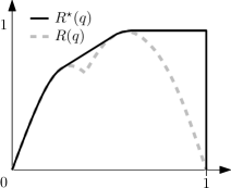
(a) Revenue curve $R(q)$ and the optimal induced revenue curve $R^{\star}(q)$.

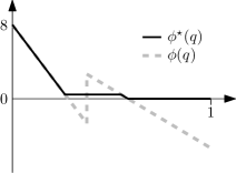
(b) Virtual value function $\varphi(q)$ and the induced virtual value function $\varphi^{\star}(q)$.

Figure 1: The dashed gray line is the revenue curve $R(q)$ and its derivative, the virtual value function $\varphi(q)$, for a irregular bimodal distribution. In black we have the curves $\varphi^{opt}$ and $R^{opt}$ corresponding to the optimal ironing interval, and optimal reserve price for this distribution. This example taken from (HartlineXX, , Chapter 3).

Revenue Curve and Quantile Space

For a value $v$ and a distribution $F$, we define the corresponding quantile as $1-F(v)$. The quantile of $v$ corresponds to the sale probability for a single bidder with valuation drawn from $F$ as the posted price $v$. Note that higher values correspond to lower quantiles. The revenue curve $R$ for value distribution $F$ is the curve, in quantile space, that is defined as $R(q)=q\cdot F^{-1}(1-q)$, see the dashed curve in Figure 1a. Myerson Myerson81 showed that the ex ante expected revenue for a bidder is $\mathbb{E}_{q\sim U[0,1]}[-R(q)\cdot y^{\prime}(q)]$, where $y$ is the interim allocation function for the standard Vickrey auction (defined formally below). The derivative of $R$ is the virtual value function $\varphi(.)$ — recall (1) — in quantile space, see Figure 1b. For regular distributions the revenue curve is concave and the virtual value function non-increasing, but for irregular distributions this is not the case.

Myerson Myerson81 showed that for any non-concave revenue curve $R$, one can create an allocation rule that will yield the same revenue as $R$’s convex hull $\mathcal{CH}(R)$. This procedure is called ironing, and for each interval where $R$ differs from $\mathcal{CH}(R)$, we take the virtual value to be slope of the convex hull over this interval. This means the virtual values are constant, and hence any two bids in that range are interchangeable, so the ironed allocation function is constant on this interval. The resulting ironed revenue curve $R^{\star}$ will be concave and the corresponding ironed virtual value function $\varphi^{\star}$ will be monotonically non-increasing. It is also useful to think of a reserve price $r$ (with corresponding quantile $q_{r}$) in a similar way, as effectively changing the virtual valuation function so that $\varphi^{\star}(q)=0$ whenever $q\geq q_{r}$ (Figure 1b), with the corresponding revenue curve $R^{\star}$ constant in that region (Figure 1a).

More generally, given any set of disjoint ironing intervals $\mathcal{I}$ and reserve price $r$, both in value space, we can imagine these modifying the revenue curve as follows. (For now this is a thought experiment; Proposition 2.1 connects these revenue curve modifications back to allocation rule modifications.) Let $R$ be the revenue curve without ironing or a reserve price, and define $R^{(\mathcal{I},r)}$ as the revenue curve induced by a set $\mathcal{I}$ of ironing intervals and reserve price $r$. This curve is defined by

$$R^{(\mathcal{I},r)}(q)=\begin{cases}R(F(r))&\text{if }q>F(r)\\ R(q_{a})+\frac{q-q_{a}}{q_{b}-q_{a}}\left(R(q_{b})-R(q_{a})\right)&\text{if }q\in(q_{a},q_{b}]\text{ with }[F^{-1}(1-q_{b}),F^{-1}(1-q_{a}))\in\mathcal{I}\\ R(q)&\text{otherwise}.\end{cases}$$ (3)

Given $\mathcal{I}$ and $r$ as above, we define the auction $A^{(\mathcal{I},r)}$ as follows: given a bid profile: (i) reject every bid with $b_{i}<r$; (ii) for each ironing interval $[a,b)\in\mathcal{I}$, treat all bids $\{b_{j}:a\leq b_{j}<b\}$ as identical (equal to some common number between $a$ and $b$); (iii) among the remaining bidders, maximize the social welfare (sum of the ironed bids of the winners); (iv) charge payments so that losers always pay 0 and so that truthful bidding is a dominant strategy for every player. This auction is well defined (i.e., independent of the choice of the common numbers in (ii)) in settings where the computation in (iii) depends only on the ordering of the ironed bids, and not on their numerical values. In this case, the payments in (iv) are uniquely defined (by standard mechanism design results). This is the case in every matroid environment and also in position auctions (see EOS07 ; V07 ). In such a setting, we use $\mathcal{A}$ to denote the set of all auctions of the form $A^{(\mathcal{I},r)}$. We restrict attention to such settings for the rest of the paper.

The Switching Trick

Given a distribution $F$, we explained two ways to use ironing intervals $\mathcal{I}$ and a reserve price $r$: (i) to define a modified revenue curve $R^{(\mathcal{I},r)}$ (and hence virtual valuations); or (ii) to define an auction $A^{(\mathcal{I},r)}$. The “switching trick” formalizes the connection between them: the expected virtual welfare of the welfare-maximizing auction with the modified virtual valuations (corresponding to the derivative of $R^{(\mathcal{I},r)}$) equals the expected virtual welfare of the modified auction $A^{(\mathcal{I},r)}$ with the original virtual valuations.

More formally, let $x_{i}:\mathbb{R}_{+}^{n}\rightarrow\mathbb{R}_{+}$ be the ex-post allocation function of the welfare maximizing truthful auction that takes the bids ${\bf b}$ of all players and results in the allocation to bidder $i$. The interim allocation function $y_{i}:[0,1]\rightarrow\mathbb{R}_{+}$ is the expected allocation to bidder $i$ when her quantile is $q$, where the expectation is over the quantiles of the other bidders: $y_{i}(q_{i})=\mathbb{E}_{{\bf q}_{-i}\sim U[0,1]^{n-1}}[x(F^{-1}(1-q),F^{-1}({\bf 1}-{\bf q}_{-i}))]$ where $F^{-1}({\bf 1}-{\bf q}_{-i})$ is ${\bf b}_{-i}$ for which each $b_{j}=F(1-q_{j})$. For example, in the standard Vickrey (single-item) auction with $n$ bidders, every bidder $i$ has the interim allocation function $y_{i}(q)=(1-q)^{n-1}$.

For every auction of the form $A^{(\mathcal{I},r)}$, the interim allocation function $y_{i}^{(\mathcal{I},r)}$ of a bidder $i$ can be expressed in terms of the interim allocation function $y_{i}$ without ironing and reserve price (see also Figure 1b):

$$y_{i}^{(\mathcal{I},r)}(q)=\begin{cases}0&\text{if }q>F(r)\\ \frac{1}{q_{b}-q_{a}}\int_{q_{a}}^{q_{b}}y(q)dq&\text{if }q\in[q_{a},q_{b})\text{ with }[F^{-1}(1-q_{b}),F^{-1}(1-q_{a}))\in\mathcal{I}\\ y_{i}(q)&\text{otherwise}.\end{cases}$$ (4)

Proposition 2.1 (Switching Trick)

Consider a matroid or position auction setting, as above. For every valuation distribution $F$, every reserve price $r$, every set $\mathcal{I}$ of disjoint ironing intervals, and every bidder $i$,

$$\mathbb{E}_{q\sim U[0,1]}[R(q)\cdot(y_{i}^{(\mathcal{I},r)})^{\prime}(q)]=\mathbb{E}_{q\sim U[0,1]}[R^{(\mathcal{I},r)}(q)\cdot y_{i}^{\prime}(q)].$$

Proof.

Fix $F$, $\mathcal{I}$, $r$, and $y$. Let $y^{(\mathcal{I},r)}$ be the interim allocation rule from running auction $A_{\mathcal{I},r}$. Let $R$ be the revenue curve of $F$ and let $R^{(\mathcal{I},r)}$ denote the revenue curve induced by $\mathcal{I}$ and $r$.

• Define a distribution $F^{(\mathcal{I},r)}$ (which is not equal to $F$ unless $\mathcal{I}=\emptyset$ and $r=0$) that has the property that its revenue curve $q\cdot F^{(\mathcal{I},r)}(1-q)$ is $R^{(\mathcal{I},r)}$. To see that this is well-defined, observe the following. Any line $\ell$ through the origin only intersects $R^{(\mathcal{I},r)}$ once (if there are point masses in $F$ then a line through the origin intersect $R$ in a single interval). This means that we can use $R^{(\mathcal{I},r)}$ to construct $F^{(\mathcal{I},r)}$: $F^{(\mathcal{I},r)}(v)$ is the $q$ for which $q\cdot v$ intersects with $R^{(\mathcal{I},r)}(q)$ (if there are any point masses then there will be a range of $q$ for which this is the case; in that case take the largest such $q$). Alternatively, see Hartline and Roughgarden HR08 for an explicit formula for $F^{(\mathcal{I},r)}$.

• If we run the same auction $A_{\mathcal{I},r}$ on bidders with values drawn from $F^{(\mathcal{I},r)}$, the expected revenue is identical to the auction with bidder values drawn from $F$:

  $$\mathbb{E}_{q\sim U[0,1]}[R(q)\cdot\left(y^{(\mathcal{I},r)}\right)^{\prime}(q)]=\mathbb{E}_{q\sim U[0,1]}[R^{(\mathcal{I},r)}(q)\cdot\left(y^{(\mathcal{I},r)}\right)^{\prime}(q)].$$

  This can easily be seen by filling in the definitions from (3) and (4).

• If the bidders have distribution $F^{(\mathcal{I},r)}$, then we might as well not iron or have a reserve price at all; so

  $$\mathbb{E}_{q\sim U[0,1]}[R^{(\mathcal{I},r)}(q)\cdot\left(y^{(\mathcal{I},r)}\right)^{\prime}(q)]=\mathbb{E}_{q\sim U[0,1]}[R^{(\mathcal{I},r)}(q)\cdot y^{\prime}(q)].$$

  This is also easily seen by filling in the definitions.

∎

2.3 Notation

In the remainder of this paper, our analysis will rely on bounding the difference in revenue of an auction with respect to the optimal auction in terms of their revenue curves. We will use the following conventions, see Table 1. The unaltered revenue curve for distribution is denoted by $R(q)=q\cdot F^{-1}(1-q)$. To denote when we use an estimator for a revenue, i.e. a revenue curve that is constructed based on samples, we use a hat: $\widehat{R}(q)=q\cdot\widehat{F^{-1}}(1-q)$. Based on the available samples we construct high-probability upper and lower bounds for $R$, that are thus denoted as $\widehat{R}_{\text{max}}(q)=q\cdot\widehat{F^{-1}}(1-q+\epsilon+\frac{1}{m})$ and $\widehat{R}_{\text{min}}(q)=q\cdot\widehat{F^{-1}}(1-q-\epsilon)$.

Revenue Curve	Description
$R$	$q\cdot F^{-1}(1-q)$
$\widehat{R}_{\text{min}}$	$q\cdot\widehat{F^{-1}}(1-q-\epsilon)$
$\widehat{R}_{\text{max}}$	$q\cdot\widehat{F^{-1}}(1-q+\epsilon+\frac{1}{m})$

Table 1: Overview of notation for revenue curves.

We use superscript to denote when a revenue curve is ironed and has a reserve price. For a general set of ironing intervals $\mathcal{I}$ and reserve price $r$, $R^{(\mathcal{I},r)}$ is the revenue curve induced by it, see (3). The superscript $\star$ denotes that the revenue curve is optimally ironed and reserved, i.e. $R^{\star}$ is the revenue curve of Myerson’s auction using $F$, and $\widehat{R}_{\text{max}}^{\star}$ is the revenue curve corresponding to the convex hull of $\widehat{R}_{\text{max}}$ that additionally stays constant after the highest point. Finally, we’ll use $R^{alg}$ and $R^{opt}$ to denote an algorithm ALG’s revenue curve and the optimal revenue curve for $F$ respectively (thus $R^{opt}=R^{\star}$, but we’ll use $R^{opt}$ to emphasize its relation to $R^{alg}$).

For the ironing intervals $\mathcal{I}$ (and reserve price $r$) we use $\mathcal{I}_{q}$ (resp. $r_{q}$) when it is important that the ironing intervals are defined in quantile space. Finally, $\mathcal{I}_{opt}$, $\mathcal{I}_{alg}$, and $\mathcal{I}_{max}$ (and similarly for reserve $r$) refer to the ironing intervals of the optimal auction, algorithm ALG and the optimal ironing intervals for $\widehat{R}_{\text{max}}$ respectively.

3 Additive Loss in Revenue for Single-Item Auctions

In this section we describe an algorithm that takes a set $X$ of $m$ samples, and a confidence parameter $\delta$ as input, and outputs a set $\mathcal{I}$ of ironing intervals and a reserve price $r$, both in value space. We focus on the case where $\mathcal{I}$ and $r$ are used in a single-item auction $A_{(1)}^{\mathcal{I},r}\in\mathcal{A}$ (recall the notation in Section 2) and show that the additive loss in revenue of $A_{(1)}^{\mathcal{I},r}$ with respect to the revenue of the optimal auction $A^{opt}_{(1)}$ for single-item auctions is $O(\epsilon\cdot n\cdot H)$, with $\epsilon=\sqrt{\frac{\ln 2\delta^{-1}}{2m}}$. In section 4 we extend the results to matroid and position auctions.

Theorem 3.1 (Main Theorem)

For a single-parameter environment with optimal auction of the form $A^{(\mathcal{I},r)}$ with $n$ i.i.d. bidders with values from unknown irregular distribution $F$, $m$ i.i.d. samples from $F$, with probability $1-\delta$, the additive loss in expected revenue of Algorithm 2 compared to the optimal expected revenue is at most $3\cdot n\cdot H\cdot\sqrt{\frac{\ln 2\delta^{-1}}{2m}}$.

3.1 The Empirical Myerson Auction

We run the Empirical Myerson auction (Algorithm 2), which we divided this into two parts: the first is an algorithm $ALG$ (Algorithm 1) that computes the ironing intervals $\mathcal{I}$ and reserve price $r$ based on samples $X$ and confidence parameter $\delta$. The second step is to run the welfare-maximizing auction subject to ironing and reservation. In this section we focus on analyzing the single-item auction, but the only place this is used is in line 2 of Algorithm 2. Auctions for position auctions and matroid environments are defined completely analogously.

• $\textnormal{ComputeAuction}(X,\delta)$
     1Construct $\widehat{F^{-1}}$ from $X$; let $\epsilon=\sqrt{\frac{\ln 2\cdot\delta^{-1}}{2|X|}}$. 2Construct $\widehat{R}_{\text{min}}(q)=q\cdot\widehat{F^{-1}}(1-q-\epsilon)$. 3Compute the convex hull $\mathcal{CH}(\widehat{R}_{\text{min}})$, of $\widehat{R}_{\text{min}}$. 4Let $\mathcal{I}_{q}$ be the set of intervals where $\widehat{R}_{\text{min}}$ and $\mathcal{CH}(\widehat{R}_{\text{min}})$ differ. 5for each quantile ironing interval $(a_{i},b_{i})\in\mathcal{I}_{q}$ 6 Add $[\widehat{F^{-1}}(1-b_{i}-\epsilon),\ \widehat{F^{-1}}(1-a_{i}-\epsilon))$ to $\mathcal{I}$. 7Let the reserve quantile be $r_{q}=\operatorname*{arg\,max}_{q}\widehat{R}_{\text{min}}(q)$. 8Let the reserve price be $r=\widehat{F^{-1}}(1-r_{q}-\epsilon)$. 9return $(\mathcal{I},r)$

Algorithm 1 Compute the ironing intervals $\mathcal{I}$ and reserve price $r$.

• $\textnormal{EmpiricalMyerson}(X,\delta,{\bf b})$
     1$\mathcal{I},r\leftarrow\textnormal{ComputeAuction}(X,\delta)$ 2return $A_{(1)}^{\mathcal{I},r}({\bf b})$

Algorithm 2 Empirical Myerson.

The Empirical Myerson auction takes an estimator for the quantile function $\widehat{F^{-1}}$ and constructs its revenue curve. From this, the convex hull $\mathcal{CH}(R)$ is computed and wherever $\mathcal{CH}(R)$ and $R$ disagree, an ironing interval is placed. Then, the highest point on $R$ is used to obtain the reserve price quantile $q_{r}=\operatorname*{arg\,max}_{q}R(q)$. Note that this is all done in quantile space, but we need to specify the reserve price and ironing intervals in value space. So the last step is to use the empirical CDF $\widehat{F}$ to obtain the values at which to place the reserve price and ironing intervals.

Algorithm 2 follows that approach, with the exception that in line 2 of ComputeAuction, we take the empirical quantile function to be $\widehat{F^{-1}}(1-q-\epsilon)$ rather than the arguably more natural choice of $\widehat{F^{-1}}(1-q)$. By the DKW inequality, $\widehat{F^{-1}}(1-q-\epsilon)\leq F^{-1}(1-q)$ with probability $1-\delta$ (we prove this in Lemma 3.3). The motivation here is to protect against overestimation — recall the cautionary tale of Example 1.2. That this approach indeed leads to good revenue guarantees is shown in this section.

3.2 Additive Revenue Loss in Terms of Revenue Curves

We start with a technical lemma that reduces bounding the loss in revenue to bounding the estimation error due to using samples as opposed to the true distribution $F$.

Lemma 3.2

For a distribution $F$, let $R^{alg}$ be the revenue curve induced by an algorithm $ALG\in\mathcal{A}$ and let $R^{opt}$ be the optimal induced revenue curve. The additive revenue loss of $ALG$ with respect to $OPT$ is at most:

$$n\cdot\max_{q\in[0,1]}\left(R^{opt}(q)-R^{alg}(q)\right).$$

Proof.

First, to calculate the ex ante expected revenue of a bidder $i$ with revenue curve $R$, ironing intervals $\mathcal{I}$ and reserve price $r$, we have by Myerson Myerson81 :

$$Rev[R,\mathcal{I},r] =-\mathbb{E}_{q\sim U[0,1]}[R(q)\cdot(y^{(\mathcal{I},r)})^{\prime}(q)].$$ (5)

Next, we apply the Switching Trick of Proposition 2.1. Let $\mathcal{I}_{alg},\mathcal{I}_{opt}$ be the sets of ironing intervals and $r_{alg},r_{opt}$ be the reserve prices of $ALG$ and $OPT$ respectively. This yields total revenues:

$$\frac{Rev[F,I_{alg},r_{alg}]}{n} =-\int_{0}^{1}R^{alg}(q)y^{\prime}(q)dq, \frac{Rev[F,I_{opt},r_{opt}]}{n} =-\int_{0}^{1}R^{opt}(q)y^{\prime}(q)dq.$$

Note that the interim allocation function $y$ in both cases is the same one; the only difference between $y^{(\mathcal{I}_{opt},r_{opt})}$ and $y^{(\mathcal{I}_{alg},r_{alg})}$ was the ironing intervals and reserve price, so after applying the switching trick, $y$ is simply the truthful welfare-maximizing interim allocation rule (for single-item auctions this is the probability for bidder $i$ to have the largest value $v_{i}=\max_{j}v_{j}$). This is the key point in our analysis, and it allows us to compare the expected revenue of both auctions directly:

$$Rev[F,\mathcal{I}_{opt},r_{opt}]-Rev[F,\mathcal{I}_{alg},r_{alg}] =n\left(-\int_{0}^{1}R^{opt}(q)y^{\prime}(q)dq+\int_{0}^{1}R^{alg}(q)y^{\prime}(q)dq\right)$$

$$=n\int_{0}^{1}\left(R^{opt}(q)-R^{alg}(q)\right)\left(-y^{\prime}(q)\right)dq$$

$$\leq n\cdot\max_{q\in[0,1]}\left(R^{opt}(q)-R^{alg}(q)\right)\cdot\int_{0}^{1}-y^{\prime}(q)dq$$

$$=n\cdot\max_{q\in[0,1]}\left(R^{opt}(q)-R^{alg}(q)\right)\cdot\left(-y(1)+y(0)\right)$$

$$=n\cdot\max_{q\in[0,1]}\left(R^{opt}(q)-R^{alg}(q)\right).$$

The inequality holds as $-y^{\prime}$ is non-negative. The last equality holds as the probability of winning when your quantile is $0$ is $y(0)=1$, and the probability of winning when your quantile is $1$ is $y(1)=0$. Rearranging the terms yields the claim. ∎

This is significant progress: the additive loss in revenue can be bounded in terms of the induced revenue curves of an algorithm ALG and the optimal algorithm, two objects that we have some hope of getting a handle on. Of course, we still need to show that the ironed revenue curve of Algorithm 2 is pointwise close to the ironed revenue curve induced by the optimal auction (Section 3.3).

3.3 Bounding the Error in the Revenue Curve

We implement the following steps to prove that the error in the learning algorithm’s estimation of the revenue curve is small.

• (Lemma 3.3) We show that we can sandwich the actual revenue curve (without ironing or reserve price) $R$ between two empirical revenue curves, $\widehat{R}_{\text{min}}$ and $\widehat{R}_{\text{max}}$ that are defined using the empirical quantile function.

• (Lemma 3.4 and Lemma 3.5) Let $\widehat{R}_{\text{max}}^{\star}$ (resp. $\widehat{R}_{\text{min}}^{\star}$) be the optimally induced revenue curve for $\widehat{R}_{\text{max}}$ (resp. $\widehat{R}_{\text{min}}$). The revenue curve induced by Algorithm 2, $R^{alg}$, is pointwise higher than the optimal induced revenue curve of the lower bound $\widehat{R}_{\text{min}}^{\star}$, and the optimal induced revenue curve for the upper bound, $\widehat{R}_{\text{max}}^{\star}$, is pointwise higher than $R^{opt}$.

• (Lemma 3.6) Finally, we show that $\widehat{R}_{\text{max}}^{\star}(q)-\widehat{R}_{\text{min}}^{\star}(q)$ is small for all $q$, and therefore the additive loss is small.

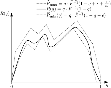
Figure 2: We can sandwich $R$ between two estimated revenue curves $\widehat{R}_{\text{min}}$ and $\widehat{R}_{\text{max}}$.

Lemma 3.3

Let $\widehat{R}_{\text{min}}(q)=q\cdot\widehat{F^{-1}}(1-q-\epsilon)$ and $\widehat{R}_{\text{max}}(q)=q\cdot\widehat{F^{-1}}(1-q+\epsilon+\frac{1}{m})$. With probability at least $1-\delta$ for all $q\in[0,1]$:

$$\widehat{R}_{\text{min}}(q)\quad\leq\quad R(q)\quad\leq\quad\widehat{R}_{\text{max}}(q).$$

Proof.

See Figure 2 for graphical intuition. We will start with the first inequality: $\widehat{R}_{\text{min}}(q)\leq R(q)$. By the DKW inequality with probability $1-\delta$ the following holds for all $v$:

$$-\epsilon\leq\widehat{F}(v)-F(v)\leq\epsilon$$ (6)

Define $q^{\prime}=F(v)$. We can rewrite the first inequality of (6):

$$q^{\prime}-\epsilon \leq\widehat{F}(v)$$

$$\widehat{F^{-1}}\left(q^{\prime}-\epsilon\right) \leq\widehat{F^{-1}}\left(\widehat{F}(v)\right)$$

Since $\widehat{F^{-1}}$ is mononotonically non-decreasing. We now invoke (2):

$$\widehat{F^{-1}}\left(q^{\prime}-\epsilon\right)\leq\widehat{F^{-1}}\left(\widehat{F}(v)\right)\leq v=F^{-1}(q^{\prime}).$$

Now let $q=1-q^{\prime}$, and multiply both sides by $q$ to obtain: $\widehat{R}_{\text{min}}(q)\leq R(q)$.

The proof for the upper bound of $R$ is analogous with the exception that we pick up another $\frac{1}{m}$ term to invoke (2). ∎

So while the the algorithm does not know the exact revenue curve $R$, it can be upper bounded by $\widehat{R}_{\text{max}}$ and lower bounded by $\widehat{R}_{\text{min}}$. We’ll use $\widehat{R}_{\text{min}}$ to give a lower bound on the revenue curve $R^{alg}$ induced by Algorithm 2, and $\widehat{R}_{\text{max}}$ to give an upper bound on the revenue curve $R^{opt}$ induced by Myerson’s optimal auction. We start with the latter.

Lemma 3.4

Let $R^{opt}$ be the optimal induced revenue curve of $R$, and let $\widehat{R}_{\text{max}}^{\star}$ be the optimal induced revenue curve for $\widehat{R}_{\text{max}}$. Then with probability $1-\delta$ for all $q\in[0,1]$:

$$R^{opt}(q)\quad\leq\quad\widehat{R}_{\text{max}}^{\star}(q).$$

Proof.

By Lemma 3.3 we know that for every $q$, $\widehat{R}_{\text{max}}(q)\geq R(q)$. First take the effect of optimally ironing both curves into account. Optimal ironing will lead to induced revenue curves $\mathcal{CH}(\widehat{R}_{\text{max}})$ and $\mathcal{CH}(R)$ and since $\widehat{R}_{\text{max}}$ is pointwise higher, so is its convex hull. What remains to be proven is that this property is maintained after the effect of the reserve price of the curve. The reserve quantile is the highest point on the curve, and the induced revenue curve will stay constant for all higher quantiles. Let $q$ be the reserve quantile for $R$. If the reserve quantile for $\widehat{R}_{\text{max}}$ happens to be the same, then the statement is proven. Moreover, if the optimal reserve quantile for $\widehat{R}_{\text{max}}$ is not $q$, it can only be higher, in which case the statement is also proven. ∎

So $\widehat{R}_{\text{max}}^{\star}$ is pointwise higher than $R^{opt}$. Proving that $\widehat{R}_{\text{min}}^{\star}$ is a lower bound for $R^{alg}$ is slightly more involved since the ironing intervals and reserve price are given by Algorithm 2, and may not be optimal. Therefore, the induced revenue curve $R^{alg}$ is in general not concave, and the reserve quantile may not be at the highest point of the curve. However, since $R^{alg}$ is induced by the reserve price and ironing intervals that were chosen by looking at $\widehat{R}_{\text{min}}$, there is enough structural information to prove the lower bound.

Lemma 3.5

Let $R^{alg}$ be the revenue curve induced by Algorithm 2 and let $\widehat{R}_{\text{min}}^{\star}$ be the optimal induced revenue curve for $\widehat{R}_{\text{min}}$. Then with probability $1-\delta$ for all $q\in[0,1]$:

$$\widehat{R}_{\text{min}}^{\star}(q)\quad\leq\quad R^{alg}(q).$$

Proof.

Again we first argue that after ironing the induced curve $\widehat{R}_{\text{min}}^{\star}$ is completely below $R^{alg}$, and subsequently show that this is still true after setting the reserve price.

Algorithm 2 picks the ironing intervals based on where $\widehat{R}_{\text{min}}^{\star}$ differs from $\mathcal{CH}(\widehat{R}_{\text{min}})$. However, $\widehat{R}_{\text{min}}$ and $R^{alg}$ are defined in quantile space, whereas the ironing intervals are defined in value space. This means that $R^{alg}$ is not necessarily ironed on the same intervals in quantile space as $\widehat{R}_{\text{min}}^{\star}$. The line that goes through the origin and intersects $\widehat{R}_{\text{min}}$ at $q$, will intersect $R$ at the point $q^{\prime}$ where the $F^{-1}(q^{\prime})=\widehat{F^{-1}}(1-q-\epsilon)$, see Figure 3. Any line through the origin intersects $\widehat{R}_{\text{min}}$ before it intersects $R$, and since ironing is done according to these lines through the origin, this property is maintained after ironing. The reserve price is determined in the same way, and hence $R^{alg}(q)\geq\widehat{R}_{\text{min}}^{\star}(q)$ for all $q\in[0,1]$ as claimed. ∎

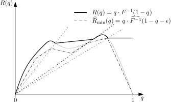
Figure 3: When we pick a value range to iron based on $\widehat{R}_{\text{min}}$, its effect on the actual revenue curve can be seen. The quantiles of the start and end point of the ironing procedure are given by the line that intersects the start and end point on $\widehat{R}_{\text{min}}$ and the origin.

So we have our upper bound and lower bounds in terms of $\widehat{F^{-1}}$. Finally we show that the difference between the two is small.

Lemma 3.6

For a distribution $F$, let $R^{alg}$ be the revenue curve induced by Algorithm 2, $R^{opt}$ be the optimal induced revenue curve. Using $m$ samples from $F$, with probability $1-\delta$ and $\epsilon=\sqrt{\frac{\ln 2\cdot\delta^{-1}}{2m}}$ for all $q$:

$$R^{opt}(q)-R^{alg}(q)\leq\widehat{R}_{\text{max}}^{\star}(q)-\widehat{R}_{\text{min}}^{\star}(q)\leq\left(2\epsilon+\frac{1}{m}\right)H\leq 3\epsilon\cdot H.$$

Proof.

Let $\mathcal{I}_{\text{max}}$ and $r_{\text{max}}$ be the set of ironing intervals and reserve price in quantile space of $\widehat{R}_{\text{max}}^{\star}$. Comparing $\widehat{R}_{\text{max}}^{\star}$ and $\widehat{R}_{\text{min}}^{\star}$ directly is difficult since the ironing intervals and reserve price may be quite different between the two. Instead, we will take the set $\mathcal{I}_{\text{max}}$ of ironing intervals $[a_{i},b_{i})$, and reserve quantile $r_{\text{max}}$ from $\widehat{R}_{\text{max}}^{\star}$ and use this to iron $\widehat{R}_{\text{min}}(q)$ at intervals $[a_{i}-2\epsilon-\frac{1}{m},b_{i}-2\epsilon-\frac{1}{m})$, and set a reserve price of $r_{\text{max}}-2\epsilon-\frac{1}{m}$.

If we compare $\widehat{R}_{\text{max}}^{\star}$ against this induced curve $\widehat{R}_{\text{min}}^{(\mathcal{I}_{\text{max}},r_{\text{max}})}$, we have an upper bound for the difference with respect to $\widehat{R}_{\text{min}}^{\star}$, since the latter is the optimal induced revenue curve and therefore pointwise higher. We can reason about ironing in quantile space without loss of generality since both $\widehat{R}_{\text{max}}$ and $\widehat{R}_{\text{min}}$ use the same function $\widehat{F^{-1}}$ (alternatively think of it as ironing in value space based on $\widehat{R}_{\text{max}}$, the line through the origin and $\widehat{R}_{\text{max}}(q)$ intersects $\widehat{R}_{\text{min}}$ at $q-2\epsilon-\frac{1}{m}$).

There are 3 cases to handle: 1) if $q$ falls in an ironing interval $[a_{i},b_{i})\in\mathcal{I}_{\text{max}}$, 2) if the quantile $q$ is higher than the reserve quantile $q\geq r_{\text{max}}$ of $\widehat{R}_{\text{max}}$, and 3) when neither of those cases apply. We start with the case for a $q$ where $\widehat{R}_{\text{max}}^{\star}(q)=\widehat{R}_{\text{max}}$, i.e. $q$ does not fall in an ironing interval and is smaller than the reserve quantile:

$$\widehat{R}_{\text{max}}^{\star}(q) =q\cdot\widehat{F^{-1}}\left(1-q+\epsilon+\frac{1}{m}\right)$$

$$\leq\left(q-2\epsilon-\frac{1}{m}\right)\cdot\widehat{F^{-1}}\left(1-q+\epsilon+\frac{1}{m}\right)+\left(2\epsilon+\frac{1}{m}\right)H$$

$$=\widehat{R}_{\text{min}}\left(q-2\epsilon-\frac{1}{m}\right)+\left(2\epsilon+\frac{1}{m}\right)H$$

$$=\widehat{R}_{\text{min}}^{\star}\left(q-2\epsilon-\frac{1}{m}\right)+\left(2\epsilon+\frac{1}{m}\right)H$$

$$\leq\widehat{R}_{\text{min}}^{\star}(q)+\left(2\epsilon+\frac{1}{m}\right)H$$

where the first inequality holds because $\widehat{F^{-1}}(q)\leq H$ for all $q$ and the last inequality follows because $\widehat{R}_{\text{min}}^{\star}$ is monotonically non-decreasing. Rearranging yields the claim for $q$ not in an ironing interval or reserved.

The other cases follow similarly: consider the case where $q\geq r_{\text{max}}$.

$$\widehat{R}_{\text{max}}^{\star}(q) =\widehat{R}_{\text{max}}\left(r_{\text{max}}\right)$$

$$=r_{\text{max}}\cdot\widehat{F^{-1}}\left(1-r_{\text{max}}+\epsilon+\frac{1}{m}\right)$$

$$\leq\left(r_{\text{max}}-2\epsilon-\frac{1}{m}\right)\cdot\widehat{F^{-1}}\left(1-r_{\text{max}}+\epsilon+\frac{1}{m}\right)+\left(2\epsilon+\frac{1}{m}\right)H$$

$$=\widehat{R}_{\text{min}}\left(r_{\text{max}}-2\epsilon-\frac{1}{m}\right)+\left(2\epsilon+\frac{1}{m}\right)H$$

$$\leq\widehat{R}_{\text{min}}^{\star}\left(r_{\text{max}}-2\epsilon-\frac{1}{m}\right)+\left(2\epsilon+\frac{1}{m}\right)H$$

$$\leq\widehat{R}_{\text{min}}^{\star}\left(q\right)+\left(2\epsilon+\frac{1}{m}\right)H$$

where the last inequality holds because $r_{\text{max}}-2\epsilon-\frac{1}{m}\leq r_{\text{max}}\leq q$ and $\widehat{R}_{\text{min}}^{\star}$ is non-decreasing.

Finally the case for when $q$ falls in an ironing interval is analogous: $\widehat{R}_{\text{max}}^{\star}(q)$ is a convex combination of the end points of the ironing interval: $\widehat{R}_{\text{max}}^{\star}(q)=\frac{q-a_{i}}{b_{i}-a_{i}}\cdot\widehat{R}_{\text{max}}(a_{i})+\left(1-\frac{q-a_{i}}{b_{i}-a_{i}}\right)\widehat{R}_{\text{max}}(b_{i})$ and hence

$$\widehat{R}_{\text{min}}^{\star}(q)\geq\frac{q-a_{i}}{b_{i}-a_{i}}\cdot\widehat{R}_{\text{min}}\left(a_{i}-2\epsilon-\frac{1}{m}\right)+\left(1-\frac{q-a_{i}}{b_{i}-a_{i}}\right)\widehat{R}_{\text{min}}\left(b_{i}-2\epsilon-\frac{1}{m}\right)+\left(2\epsilon+\frac{1}{m}\right)H.$$

And so $\widehat{R}_{\text{max}}^{\star}(q)-\widehat{R}_{\text{min}}^{\star}(q)\leq\left(2\epsilon+\frac{1}{m}\right)H$ in all cases. ∎

Theorem 3.1 now follows by combining Lemmas 3.2 and 3.6. The additive loss the in expected revenue of Algorithm 2 is at most $3\epsilon\cdot n\cdot H$.

Proof of Theorem 3.1: By Lemma 3.2 we can express the total additive error of the expected revenue of an algorithm that yields ironing intervals $\mathcal{I}_{alg}$ and reserve price $r_{alg}$ with respect to the optimal auction as:

$$\frac{Rev[F,\mathcal{I}_{opt},r_{opt}]-Rev[F,\mathcal{I}_{alg},r_{alg}]}{n}\leq\max_{q\in[0,1]}\left(R^{opt}(q)-R^{alg}(q)\right).$$

By Lemma 3.6, Algorithm 2 yields

$$\max_{q\in[0,1]}\left(R^{opt}(q)-R^{alg}(q)\right)\leq\left(2\epsilon+\frac{1}{m}\right)H.$$

The theorem follows. $\blacksquare$

When valuations lie in $[1,H]$, so that the optimal expected revenue is bounded below, these results easily imply a sample complexity upper bound $O\left(\epsilon^{-2}\ln\epsilon^{-1}n^{2}H^{2}\right)$ for learning (efficiently) a $(1-\epsilon)$-(multiplicative) approximate auction.

In Section 4 we show how to extend these results from single-item auctions to matroid environments and position environments.

4 Matroid and Position Environments

In Lemma 3.2 we showed that for environments with optimal auctions in $\mathcal{A}_{\mathcal{I},r}$, the additive loss of Algorithm 2 can be bounded in terms of the error in estimating the ironed revenue curve.

In this section we show that Myerson’s optimal auction can be expressed in this way for more general single-parameter environments with i.i.d. bidders as well: namely in position auctions and auctions with matroid constraints. The theorem statement is as follows; the proof follows from Fact 4.2 and Fact 4.3 that show that the optimal auctions for those environments are in $\mathcal{A}$ (i.e., have the form $A^{(\mathcal{I},r)}$ for a suitable choice of ironed intervals $\mathcal{I}$ and reserve price $r$).

Theorem 4.1

For position and matroid auctions with $n$ i.i.d. bidders with values from unknown distribution $F$, $m$ i.i.d. samples from $F$, with probability $1-\delta$, the additive loss in expected revenue of Algorithm 2 compared to the optimal expected revenue is at most $3\cdot n\cdot H\cdot\sqrt{\frac{\ln 2\delta^{-1}}{2m}}$.

Our results stand in contrast to previous work on picking the optimal reserve price based on samples, for which a $\Omega(\frac{\log n}{\log\log n})$ lower bound is known in these settings (Devanur14, ).

4.1 Position Auctions

A position auction (V07, ) is one where the winners are given a position, and position $i$ comes with a certain quantity $x_{i}$ of the good. The canonical example is that of ad slot auctions for sponsored search, where the best slot has the highest click-through-rate, and subsequent slots have lower and lower click-through-rates. In an optimal auction, the bidder with the highest ironed virtual value gets the best slot, the second highest ironed virtual value the second slot, and so on.

Fact 4.2

The optimal auction $A_{(pos)}^{opt}$ for position auctions can be expressed as an auction with ironing and reserve price in value space: $A_{(pos)}^{opt}\in\mathcal{A}$.

Proof.

In the optimal auction, the bidder with the highest ironed virtual value is awarded the first position (with allocation $x_{1}$), the bidder with the second highest ironed virtual value the second position with $x_{2}$, and so on. Since the ironed virtual value are monotonically non-decreasing in the value of a bidder, and identical in ironing intervals, this can equivalently be described by an auction in $\mathcal{A}$. ∎

4.2 Matroid Environments

In a matroid environment, the feasible allocations are given by matroid $\mathcal{M}=(E,I)$, where $E$ are the players and $I$ are independent sets. The auction can simultaneously serve only sets $S$ of players that form an independent set of the matroid $S\in I$. A special case of this is the rank $k$ uniform matroid, which accepts all subsets of size at most $k$, i.e. it is a $k$-unit auction environment.

In matroid environments, the ex-post allocation function $x_{i}(\bf b)$ and interim allocation function $y_{i}(q)$ are no longer the same for each player, e.g. imagine a player $i$ who is not part of any independent set, then $y(q)=0$ everywhere. So for matroid environments, the total additive loss is

$$Rev[F,\mathcal{I}_{opt},r_{opt}]-Rev[F,\mathcal{I}_{alg},r_{alg}] =\sum_{i=1}^{n}\left(-\int_{0}^{1}R^{opt}(q)y_{i}^{\prime}(q)dq+\int_{0}^{1}R^{alg}(q)y_{i}^{\prime}(q)dq\right)$$

$$=...$$

$$=n\cdot\max_{q\in[0,1]}\left(R^{opt}(q)-R^{alg}(q)\right).$$

We need to show that the optimal allocation can still be expressed in terms of an auction $A\in\mathcal{A}$.

Fact 4.3

The optimal auction $A_{(mat)}^{opt}$ for matroid auctions can be expressed as an auction with ironing and reserve price in value space: $A_{(pos)}^{opt}\in\mathcal{A}$.

Proof of Fact 4.3: A property of matroids is that the following simple greedy algorithm yields the optimal solution:

• $\textnormal{Greedy}(E,I)$
     1$S\leftarrow\emptyset$ 2while $\{i:i\not\in S\land S\cup\{i\}\in I\}\neq\emptyset$ 3 $S\leftarrow\operatorname*{arg\,max}\{v_{i}:i\not\in S\land S\cup\{i\}\in I\}$ 4return $S$

where $v_{i}$ is the (ironed virtual) value associated with bidder $i$. Since the order of largest values is the same for both virtual values and bids (up to ties), the allocation of the optimal auction is identical to the auction that irons on $\mathcal{I}_{opt}$ and has reserve price $r_{opt}$ (up to tie-braking); hence $A_{(mat)}^{opt}\in\mathcal{A}$. $\blacksquare$

5 No-Regret Algorithm

So far we assumed access to batch of samples before having to choose an auction. In this section we show that even if we start out without any samples, but run the auction is a repeated setting, using past bids as samples leads to a no-regret algorithm. The goal here is to achieve additive error $o(T)\cdot O(\text{poly}(n,H,\delta))$ — the error can be polynomial in all parameters except the time horizon $T$, for which it should be strictly sublinear. We show that for Algorithm 3 the total loss grows as $\widetilde{O}(\sqrt{T}\sqrt{n}\sqrt{\log(\delta^{-1})}H)$ and hence results in a no-regret algorithm.

• $\textnormal{No-Regret-Auction}(\delta,T)$
     1$\rhd$ Round 0: 2Collect a set of bids $\bf b$, run $\textnormal{VCG}(\bf b)$ 3$X\leftarrow\bf b$ 4for round $t=1...T$ 5 Collect a set of bids $\bf b$ 6 $\textnormal{EmpiricalMyerson}(X,\delta/T,\bf b)$ 7 $X\leftarrow X\cup\bf b$

Algorithm 3 A no-regret algorithm for optimal auctions.

Invoking Theorem 3.1 with confidence parameter $\delta/T$ and taking a union bound, we have the following.

Fact 5.1

With probability $1-\delta$, for all rounds simultaneously, each round $t\in[1,T]$ of Algorithm 3 has additive loss at most $3\sqrt{\frac{\ln(2T\delta^{-1})}{2nt}}\cdot n\cdot H$.

This leads to the following no-regret bound.

Theorem 5.2

With probability $1-\delta$, the total additive loss of Algorithm 3 is $O(\sqrt{n}\sqrt{T\log T}\sqrt{\log\delta^{-1}}\cdot H)$, which is $\widetilde{O}(T^{1/2})$ with respect to $T$.

Proof.

By Fact 5.1 with probability $1-\delta$ for all rounds simultaneously, the additive loss for round $t$ is bounded by $3\sqrt{\frac{\ln(2T\delta^{-1})}{2nt}}\cdot n\cdot H$. The loss of day 0 is at most $H\cdot n$. The total loss can then be bounded by:

$$(n\cdot H)\cdot\left(1+3\sum_{t=1}^{T}\sqrt{\frac{\ln(2T\delta^{-1})}{2nt}}\right)$$

We can rewrite the sum:

$$\sum_{t=1}^{T}\sqrt{\frac{\ln(2T/\delta)}{2nt}} =\sqrt{\frac{\ln(2T/\delta)}{2n}}\cdot\sum_{t=1}^{T}\sqrt{\frac{1}{t}}$$

$$\leq\sqrt{\frac{\ln(2T/\delta)}{2n}}\cdot 2\sqrt{T}$$

$$=\sqrt{\frac{2T\ln(2T/\delta)}{n}}$$

Hence the total loss is

$$(n\cdot H)\cdot\left(1+3\sqrt{\frac{2T\ln(4T/\delta)}{n}}\right)=O(\sqrt{n}\sqrt{T\log T}\sqrt{\log\delta^{-1}}\cdot H);$$

the dependence on $T$ is $O(\sqrt{T\log T})=\widetilde{O}(\sqrt{T})$. ∎

The bound of $O(\sqrt{T\log T})$ is almost tight, as there is a lower bound of $\Omega(\sqrt{T})$ given by Cesa-Bianchi13 . Also note that if we do not know $T$ a priori, we can use a standard doubling argument to obtain the same asymptotic guarantee.

Appendix A Reduced Information Model

This appendix considers a reduced information model for i.i.d. bidders where the auctioneer can only set a reserve price and then observes the selling price; see also [6]. The goal is to model an observer who can see the outcome of past auctions, and perhaps submit a “shill bid” to set a reserve, but cannot directly observe the bids.

We assume we observe $m$ samples from the second highest order statistic (so out of $n$ i.i.d. bids, we see the second highest bid). We show that there are distributions such that, in order to get the performance close to that of running Myerson in the reduced information model, you first need to see at least an exponential number of samples. This is far more than what would be needed with regular valuation distributions, where only the monopoly price is relevant.

A.1 Lower Bound

Theorem A.1

For any $\epsilon>0$, to obtain $\frac{1}{4}-\epsilon$ additive loss compared to Myerson’s auction, with constant probability you need $\Omega(2^{n}/n)$ samples from $F_{(2)}$.

Before proving the statement, let’s think about what this means: it means that if all we observe are samples from $F_{(2)}$, for large $n$, we cannot hope to get a vanishing regret in a polynomial (in $n$) number of steps. Moreover, on this distribution, Myerson obtains at most 2 expected revenue, so we lose $\frac{1}{8}$ of the profit (see corollary after the proof).

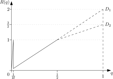
(a) Two distributions, $D_{1}$ and $D_{2}$ that are hard to distinguish using samples from $F_{(2)}$. The distributions agree on $q\in[0,1/2]$ and disagree elsewhere.

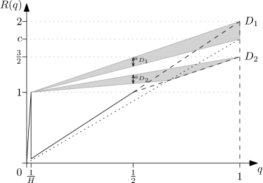
(b) Consider ironing on $[c,H)$. The top shaded area indicates the loss with respect to $D_{1}$ and the bottom shaded area represents the loss with respect to $D_{2}$.

Figure 4: Lower bound example for optimal auctions using samples from $F_{(2)}$.

Proof of Theorem A.1: We’ll give 2 distributions, $D_{1}$ and $D_{2}$, such that we need $\Omega(2^{n})$ samples from $F_{(2)}$ to differentiate between the two. Moreover, we’ll show that every auction that approximates the optimal auction for either $D_{1}$ or $D_{2}$, incurs an additive loss of at least $\frac{1}{2}(1-\frac{1}{\sqrt{2}})$ on one of the two.

We define $D_{1}$ and $D_{2}$ by their quantile function:

$$D^{-1}_{1}(q) =\begin{cases}H&\text{for }q\leq\frac{1}{H}\\ 2&\text{otherwise}\end{cases}$$

$$D^{-1}_{2}(q) =\begin{cases}H&\text{for }q\leq\frac{1}{H}\\ 2&\text{for }\frac{1}{H}<q\leq\frac{1}{2}\\ 1+\frac{1}{2q}&\text{otherwise}.\end{cases}$$

Here $H\gg n$ is a sufficiently large constant. The two distributions agree on $q\in[0,\frac{1}{2}]$. For $q\in(\frac{1}{2},1]$ they differ, and the effect on the revenue curve can be seen in Figure 4a.

To complete the proof we need to show 2 things: 1) that differentiating between $D_{1}$ and $D_{2}$ based on samples from $F_{(2)}$ requires $\Omega(2^{n}/2)$ samples, and 2) that no auction can simultaneously approximate the optimal solution for both.

The first aspect of this is straightforward. Whenever we observe a sample from $F_{(2)}$ from the top half quantile: $q\in[0,\frac{1}{2}]$, we get no information, since this is the same for both distributions. So a necessary condition for differentiating between $D_{1}$ and $D_{2}$ is if we observe a sample from $q\in(\frac{1}{2},1]$. For this to happen, we need that out of $n$ draws, $n-1$ draws are in the bottom quantile. This happens with probability $\frac{n}{2^{n-1}}$, so after $\frac{2^{n}}{n}$ samples, with probability approximately $1-\frac{1}{e}$ we haven’t seen a sample that will differentiate the two distributions.

Now we will show that until the moment when you can differentiate between $D_{1}$ and $D_{2}$, there is no way to run an auction that performs well for both. Note that the optimal auction for $D_{1}$ is to iron $[2,H)$ and the optimal auction for $D_{2}$ is to iron $[\frac{3}{2},H)$. Neither has a reserve price. The set of all auctions that could potentially work well for either, is the set of auctions that irons $[c,H)$ (see Figure 4b).

We’ll only count the loss we incur in the range $[0,\frac{1}{2}]$, take $H\rightarrow\infty$ and we see that if $a$ is the height of the shaded region (of $D_{1}$ resp. $D_{2}$) at $q=\frac{1}{2}$, then its loss with respect to the optimal auction is:

$$n\cdot\int_{0}^{\frac{1}{2}}2aq\cdot(n-1)(1-q)^{n-2}dq =\left[2anq(1-q)^{n-1}\right]_{0}^{1/2}-2an\int_{0}^{\frac{1}{2}}(1-q)^{n-1}dq$$

$$=2an\left(\frac{1}{2}\right)^{n-1}-2an\left[\frac{1}{n}(1-q)^{n}\right]_{0}^{1/2}$$

$$=2an\left(\frac{1}{2}\right)^{n-1}-2an\frac{1}{n}\left(\frac{1}{2}\right)^{n}+2an\frac{1}{n}$$

$$=2an\left(\frac{1}{2}\right)^{n-1}\left(1-\frac{1}{2n}\right)+2a$$

$$\geq 2a$$

This means, that if we can show that for all choices of $c\in[3/2,1]$ at least one of $D_{1},D_{2}$ has a large $a$, we are done. The closer $c$ is to $2$, the smaller $a_{D_{2}}$ is, the closer $c$ is to $3/2$, the smaller $a_{D_{1}}$, so we’ll balance the two and show that neither is small enough.

Finding $a_{D_{1}}$ in terms of $c$ is easy enough: $a_{D_{1}}=\frac{2-c}{2}$. $a_{D_{2}}$ is slightly harder: we first need to find the intersection of $q\cdot c$ and $R_{D_{2}}(q)$:

$$\frac{1}{2}+q =qc$$

$$(c-1)q =\frac{1}{2}$$

$$q =\frac{1}{2(c-1)}$$

So the lower part of the shaded area of $D_{2}$ is a line that passes through the points $(0,1)$ and $(\frac{1}{2(c-1)},\frac{c}{2(c-1)})$. The line segment that connects the two is given by the equation $1+q(2-c)$ hence at $q=\frac{1}{2}$ it is $2-c/2$, therefore $a_{D_{2}}=\frac{5}{4}-2+\frac{c}{2}=\frac{c}{2}-\frac{3}{4}$.

Setting $a_{D_{1}}=a_{D_{2}}$ yields $c=\frac{7}{4}$ with $a_{D_{1}}=a_{D_{2}}=\frac{1}{8}$. Therefore, for any auction that we decide to run will have additive loss of $2a=\frac{1}{4}$ on one of the two distributions, and we need $\Omega(2^{n}/n)$ samples to decide which distribution we are dealing with. $\blacksquare$

Corollary A.2

For any $\epsilon>0$, to obtain a $(\frac{7}{8}+\epsilon)$-approximation (multiplicative) to Myerson’s auction, with constant probability you need $\Omega(2^{n}/n)$ samples.

Proof.

We can upper bound the revenue curve by the constant $2$, to show that the optimal auction cannot have expected revenue more than $2$. Since we have additive loss of $1/4$, the multiplicative approximation ratio is at most $\frac{7}{8}$. ∎

References

- [1] Pablo Daniel Azar, Constantinos Daskalakis, Silvio Micali, and S. Matthew Weinberg. Optimal and efficient parametric auctions. In Proceedings of the Twenty-Fourth Annual ACM-SIAM Symposium on Discrete Algorithms, SODA 2013, New Orleans, Louisiana, USA, January 6-8, 2013, pages 596–604, 2013.
- [2] Moshe Babaioff, Liad Blumrosen, Shaddin Dughmi, and Yaron Singer. Posting prices with unknown distributions. In Innovations in Computer Science (ICS). Tsinghua University Press, January 2011.
- [3] Maria-Florina Balcan, Avrim Blum, Jason D. Hartline, and Yishay Mansour. Reducing mechanism design to algorithm design via machine learning. J. Comput. Syst. Sci., 74(8):1245–1270, 2008.
- [4] S. Baliga and R. Vohra. Market research and market design. Advances in Theoretical Economics, 3, 2003. Article 5.
- [5] N. Cesa-Bianchi, C. Gentile, and Y. Mansour. Regret minimization for reserve prices in second-price auctions. IEEE Transactions on Information Theory, 61(1):549–564, 2015.
- [6] Nicolò Cesa-Bianchi, Claudio Gentile, and Yishay Mansour. Regret minimization for reserve prices in second-price auctions. In Proceedings of the Twenty-Fourth Annual ACM-SIAM Symposium on Discrete Algorithms, SODA ’13, pages 1190–1204. SIAM, 2013.
- [7] Shuchi Chawla, Jason D. Hartline, and Denis Nekipelov. Mechanism design for data science. CoRR, abs/1404.5971, 2014.
- [8] Alessandro Chiesa, Silvio Micali, and Zeyuan Allen Zhu. Mechanism design with approximate valuations. In Innovations in Theoretical Computer Science 2012, Cambridge, MA, USA, January 8-10, 2012, pages 34–38, 2012.
- [9] Richard Cole and Tim Roughgarden. The sample complexity of revenue maximization. In Proceedings of the 46th Annual ACM Symposium on Theory of Computing, pages 243–252. ACM, 2014.
- [10] Jacques Crémer and Richard P. McLean. Optimal selling strategies under uncertainty for a discriminating monopolist when demands are interdependent. Econometrica, 53(2):345–361, 1985.
- [11] Nikhil R Devanur, Jason D Hartline, and Qiqi Yan. Envy freedom and prior-free mechanism design. Journal of Economic Theory, 2014.
- [12] Peerapong Dhangwatnotai, Tim Roughgarden, and Qiqi Yan. Revenue maximization with a single sample. In Proceedings of the 11th ACM Conference on Electronic Commerce (EC), pages 129–138, 2010.
- [13] S. Dughmi, L. Han, and N. Nisan. Sampling and representation complexity of revenue maximization. In Workshop on Internet and Network Economics (WINE), pages 277–291, 2014.
- [14] Aryeh Dvoretzky, Jack Kiefer, and Jacob Wolfowitz. Asymptotic minimax character of the sample distribution function and of the classical multinomial estimator. The Annals of Mathematical Statistics, pages 642–669, 1956.
- [15] Benjamin Edelman, Michael Ostrovsky, and Michael Schwarz. Internet advertising and the generalized second-price auction: Selling billions of dollars worth of keywords. American Economic Review, 97(1):242–259, 2007.
- [16] Edith Elkind. Designing and learning optimal finite support auctions. In Proceedings of the eighteenth annual ACM-SIAM symposium on Discrete algorithms, pages 736–745. SIAM, 2007.
- [17] Hu Fu, Nima Haghpanah, Jason D. Hartline, and Robert Kleinberg. Optimal auctions for correlated buyers with sampling. In EC, pages 23–36, 2014.
- [18] Andrew V Goldberg, Jason D Hartline, Anna R Karlin, Michael Saks, and Andrew Wright. Competitive auctions. Games and Economic Behavior, 55(2):242–269, 2006.
- [19] Bach Q Ha and Jason D Hartline. Mechanism design via consensus estimates, cross checking, and profit extraction. ACM Transactions on Economics and Computation, 1(2):8, 2013.
- [20] Jason Hartline. Mechanism design and approximation. Book draft (September 2014), September 2014.
- [21] Jason D Hartline and Tim Roughgarden. Optimal mechanism design and money burning. In Proceedings of the fortieth annual ACM symposium on Theory of computing, pages 75–84. ACM, 2008.
- [22] Zhiyi Huang, Yishay Mansour, and Tim Roughgarden. Making the most of your samples. Proceedings of EC’15, 2015.
- [23] Robert D. Kleinberg and Frank Thomson Leighton. The value of knowing a demand curve: Bounds on regret for online posted-price auctions. In FOCS, pages 594–605, New York, New York, USA., 2003. IEEE Computer Society.
- [24] Pascal Massart. The tight constant in the Dvoretzky-Kiefer-Wolfowitz inequality. The Annals of Probability, pages 1269–1283, 1990.
- [25] Andres Munoz Medina and Mehryar Mohri. Learning theory and algorithms for revenue optimization in second price auctions with reserve. In Proceedings of The 31st Intl. Conf. on Machine Learning, pages 262–270, 2014.
- [26] J. Morgenstern and T. Roughgarden. The psuedo-dimension of near-optimal auctions. To appear in NIPS ’16, 2015.
- [27] Roger B Myerson. Optimal auction design. Mathematics of operations research, 6(1):58–73, 1981.
- [28] Z. Neeman. The effectiveness of English auctions. Games and Economic Behavior, 43(2):214–238, 2003.
- [29] Noam Nisan. Introduction to mechanism design (for computer scientists). In Noam Nisan, Tim Roughgarden, Eva Tardos, and Vijay Vazirani, editors, Algorithmic Game Theory. Cambridge University Press, 2007.
- [30] I. Segal. Optimal pricing mechanisms with unknown demand. American Economic Review, 93(3):509–529, 2003.
- [31] Balasubramanian Sivan and Vasilis Syrgkanis. Vickrey auctions for irregular distributions. In Web and Internet Economics, pages 422–435. Springer, 2013.
- [32] Leslie G Valiant. A theory of the learnable. Communications of the ACM, 27(11):1134–1142, 1984.
- [33] Hal R Varian. Position auctions. international Journal of industrial Organization, 25(6):1163–1178, 2007.