An identifiability problem in a state model for partly undetected chronic diseases

Abstract

Recently, we proposed an state model (compartment model) to describe the progression of a chronic disease with an pre-clinical (“undiagnosed”) state before clinical diagnosis. It is an open question, if a sequence of cross-sectional studies with mortality follow-up is sufficient to estimate the true incidence rate of the disease, i.e. the incidence of the undiagnosed and diagnosed disease. In this note, we construct a counterexample and show that this cannot be achieved in general.

1 Introduction

1.1 Compartment model

Recently, we introduced a compartment model with a pre-clinical stage preceding the clinical stage [1]. The model involves calendar time $t$, and the different ages $a$ of the subjects in the population. The transition rates between the states are denoted as in Figure 1.

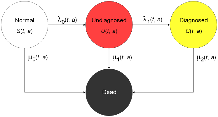
Figure 1: Chronic disease model with four states and the corresponding transition rates. People in the state Normal are healthy with respect to the disease under consideration. After onset of the disease, they change to state Undiagnosed and maybe later to the state Diagnosed. The absorbing state Dead can be reached from all other states. The numbers of persons in the states and the transition rates depend on calendar time $t$ and age $a.$

Using the definition $N(t,a)=S(t,a)+U(t,a)+C(t,a)$ and setting

$$p_{0}(t,a) =\frac{S(t,a)}{N(t,a)}$$

$$p_{1}(t,a) =\frac{U(t,a)}{N(t,a)}$$

$$p_{2}(t,a) =\frac{C(t,a)}{N(t,a)},$$

the compartment model in Figure 1 is governed by a system of partial differential equations (PDEs):

(1) $$(\partial_{t}+\partial_{a})p_{1} =-\bigl{(}\lambda_{0}+\lambda_{1}+\mu_{1}-\mu\bigr{)}\,p_{1}-\lambda_{0}\,p_{2}+\lambda_{0}$$

(2) $$(\partial_{t}+\partial_{a})p_{2} =\lambda_{1}\,p_{1}-\bigl{(}\mu_{2}-\mu\bigr{)}\,p_{2}.$$

For brevity we have written $\partial_{x}=\frac{\partial}{\partial x},~{}x\in\{t,a\}.$ In Eq. (1) – (2) the general mortality $\mu$ is given by

(3) $$\mu=p_{0}\mu_{0}+p_{1}\mu_{1}+p_{2}\mu_{2}.$$

Together with the initial conditions $p_{1}(t,0)=p_{2}(t,0)=0$ for all $t,$ the system (1) – (2) completely describes the temporal dynamics of the disease in the considered population. The quantity $p_{0}$ can be obtained by

(4) $$p_{0}=1-p_{1}-p_{2}.$$

1.2 Direct and inverse problem

Assumed that the functions $\lambda_{0},\lambda_{1},\mu_{1},\mu_{2},\mu$ on the right-hand sides of system (1) – (2) are suffiently smooth, then the associated initial value problem $p_{1}(t,0)=p_{2}(t,0)=0$ for all $t$ has a unique solution. This means that together with the initial condition, there is a function

(5) $$\Phi:\Theta=\bigl{(}\lambda_{0},\lambda_{1},\mu_{1},\mu_{2},\mu\bigr{)}\mapsto P=(p_{1},p_{2}).$$

Given the initial conditions, the operator $\Phi$ maps the transition rates $\Theta$ onto the uniquely associated prevalence functions $\Phi(\Theta)=P=(p_{1},p_{2}).$ This problem is called the direct problem or forward problem [2].

Similar to the simpler compartment model in [3], the question arises if and under which circumstances the opposite way is possible. Does a series prevalence studies $P$ allow to estimate the transition rates $\Theta$? Mathematically, this problem is expressed as inversion of the function $\Phi$. Given $P,$ the question is if there is a unique $\Theta$ such that $\Phi(\Theta)=P?$ The problem of estimating the rates from prevalence data, is called an inverse problem [2]. It is not guaranteed that the inverse problem has a solution. Examination of conditions such that the inverse problem has a solution is called the analysis of identifiability [4].

Under certain circumstances, the operator $\Phi$ is indeed invertible. Assumed that the mortality rates $\mu_{1},\mu_{2},$ and $\mu$ are known, then for given $P=(p_{1},p_{2})$ the system (1) – (2) can be solved for $\lambda_{0}$ and $\lambda_{1}.$ Thus, in these cases $\Phi$ is invertible.

In the next section, we will show that is not always the case.

2 Identifiability problem

We consider two prevalence studies at calendar times $t_{1}<t_{2}$ with mortality follow-up. This means, on the one hand we have estimates for the age courses of the prevalences $p_{1}$ and $p_{2}$ at $t_{1}$ and $t_{2}.$ On the other hand, we have additional information if and when any participant at $t_{1}$ has died before $t_{2}.$

Let us assume that for any participant who deceased between $t_{1}$ and $t_{2}$, we do not have information about what state the person was in at the time of death. For example, a person who was in the Normal state at $t_{1}$ and died before $t_{2}$ could have deceased when he was still in the Normal state, in the Undiagnosed state or in the Diagnosed state. An exception is someone dying between $t_{1}$ and $t_{2}$, who was in the Diagnosed state. As the Diagnosed state can only be left via the transition to Dead state, the information from the mortality follow-up helps to estimate $\mu_{2}.$ Thus, the mortality follow-up contributes to estimate the general mortality $\mu$ or occasionally the mortality $\mu_{2}$, but not to estimate $\mu_{0}$ or $\mu_{1}.$

The question arises: Given $p_{k}(t_{j},\cdot),~{}j,k=1,2,~{}\mu(t^{\star},\cdot)$ and $\mu_{2}(t^{\star},\cdot)$ for some $t^{\star}$ with $t_{1}<t^{\star}<t_{2},$ are we able to estimate the rates $\lambda_{0},\lambda_{1},\mu_{0},$ and $\mu_{1}$ at $t^{\star}?$ In the following we will show that this is not the case. This is done by constructing a counterexample with given $p_{1},p_{2},\mu,\mu_{2}$ but different $\lambda_{0},\lambda_{1},\mu_{0},$ and $\mu_{1}.$

Consider the system (1) – (2) being in equilibrium such that $\partial_{t}\,p_{k}(t^{\star},a)=\partial_{a}\,p_{k}(t^{\star},a)=0,~{}k=1,2,$ for all $a.$ Furthermore, let $p_{0}=0.5,p_{1}=0.3$ and $p_{2}=0.2,\mu=0.6,\mu_{2}=0.8.$ Obviously, it holds $p_{0}+p_{1}+p_{2}=1.$ From $\partial_{x}p_{2}=0,~{}x\in\{t,a\}$ it follows that $\lambda_{1}=(\mu_{2}-\mu)\tfrac{p_{2}}{p_{1}}=\tfrac{4}{30}.$ If we choose $\mu_{1}^{(1)}=0.5$ and $\mu_{1}^{(2)}=0.6,$ then from $\mu=p_{0}\mu_{0}+p_{1}\mu_{1}+p_{2}\mu_{2}$ it follows that $\mu_{0}^{(1)}=0.58$ and $\mu_{0}^{(2)}=0.52.$ In addition, $\partial_{x}p_{1}=0,~{}x\in\{t,a\}$ implies $\lambda_{0}=(\lambda_{1}+\mu_{1}-\mu)\tfrac{p_{1}}{p_{0}}.$ Thus, it holds $\lambda_{0}^{(1)}=0.02$ and $\lambda_{0}^{(2)}=0.08.$ The results are summarized in Table 1.

Variable	Value 1	Value 2
$p_{0}$	0.5
$p_{1}$	0.3
$p_{2}$	0.2
$\mu$	0.6
$\mu_{2}$	0.8
$\lambda_{1}$	$\nicefrac{{4}}{{30}}$
$\mu_{1}$	0.5	0.6
$\mu_{0}$	0.58	0.52
$\lambda_{0}$	0.02	0.08

Table 1: Example for non-identifiability of the system (1) – (4). In an equilibrium state ($\partial_{x}p_{k}=0,~{}k=1,2,~{}x\in\{t,a\}$), measured values in the upper half of the table are consistent with the values in the lower half.

Hence, from given $p_{1},p_{2},\mu,\mu_{2},$ in equilibrium, we were able to construct different $\lambda_{0},\lambda_{1},\mu_{0},$ and $\mu_{1},$ which are consistent with the system (1) – (4). This implies that two cross-sections at $t_{1}$ and $t_{2}$ with mortality follow-up are not sufficient to make the system identifiable.

3 Conclusion

In this technical note it was shown by a counterexample that two cross-sectional studies with mortality follow-up are not sufficient to make the system (1) – (4) identifiable. This means, from two cross-sectional studies and measured $p_{k},~{}k=0,1,2,$ and known $\mu,\mu_{2}$ it is not possible to estimate the incidence rates $\lambda_{0}$ and $\lambda_{1}.$

The counterexample was constructed by the system (1) – (2) being in equilibrium. This is not a loss of generalizability. It is sufficient to find one example of non-identifiability to prove non-existence of a solution of the inverse problem.

Note that from measured $p_{k},~{}k=0,1,2,$ and known $\mu,\mu_{2},$ the rate $\lambda_{1}$ is estimable. This can be seen by solving Eq. (2) for $\lambda_{1}.$

Contact:
Ralph Brinks
German Diabetes Center
Auf’m Hennekamp 65
D- 40225 Duesseldorf
ralph.brinks@ddz.uni-duesseldorf.de

References

• [1] Brinks R, Bardenheier BH, Hoyer A, Lin J, Landwehr S, Gregg EW. Development and demonstration of a state model for the estimation of incidence of partly undetected chronic diseases. BMC Medical Research Methodology. 2015;15(1):98.
• [2] Aster RC, Borchers B, Thurber CH. Parameter estimation and inverse problems. Academic Press; 2011.
• [3] Brinks R, Landwehr S. A new relation between prevalence and incidence of a chronic disease. Mathematical Medicine and Biology. 2015;.
• [4] Eisenfeld J. A simple solution to the compartmental structural-indentifiability problem. Mathematical Biosciences. 1986;79(2):209–220.