Black Holes with Scalar Hairs in Einstein-Gauss-Bonnet Gravity

Abstract

The Einstein-Gauss-Bonnet gravity in five dimensions is extended by scalar fields and the corresponding equations are reduced to a system of non-linear differential equations. A large family of regular solutions of these equations is shown to exist. Generically, these solutions are spinning black holes with scalar hairs. They can be characterized (but not uniquely) by an horizon and an angular velocity on this horizon. Taking particular limits the black holes approach boson star or become extremal, in any case the limiting configurations remain hairy.

PACS Numbers: 04.70.-s, 04.50.Gh, 11.25.Tq

1 Introduction

Much attention was devoted during the recent years to gravity theories supplemented by scalar fields. There are several reasons for that : scalar fields appear as fundamental constituents in the standard model of particle physics as well as in numerous models attempting to go beyond this well tested theory. Bypassing the long standing ’No Hair Theorem’, black holes solutions with scalar hairs have been constructed in [1], [2]. These new solutions of the Einstein-Klein-Gordon equations were constructed for a single massive complex scalar field and exist provide the black hole rotates sufficiently fast; as so they provide hairy generalizations of Kerr black holes. The influence of a self-gravitating potential on these solutions was studied in [3].

Among the numerous theoretical ideas explored to encompass the standard model and, hopefully, to improve our understanding of the Universe, models formulated in more than four dimensional space-times emerge as promising candidates. Progressively they motivate the study of general relativity in $d$ dimensions. The understanding of the gravitational interaction in higher dimensions and the classification of the underlying classical solutions, like black holes and other compact objects, constitue a research topic by itself. Even in the vacuum, the richness of the solutions available in $d$ dimensions [4] is remarkable. In particular the black holes are characterized by $[(d-1)/2]$ independent angular momenta. For odd number of dimensions, spinning solutions with all equal angular momentum present an enhanced symmetry, the underlying equations can be set in co-dimension one problem allowing for simplifications in the more elaborated dynamical equations. This feature can be used, in some circumstances, to study some dynamical processes, (e.g. collapsing shells in rotations [5]). Some calculations can be performed more easily in a space-time with five -rather than four- dimensions.

The construction of hairy black holes in higher dimensions therefore appeared as a natural continuation of the work [1] and it was the object of [6]. In that paper it was shown that Myers-Perry black holes with scalar hairs exist on a specific domain of the two-dimensional parameter space of the problem : the black hole horizon and the angular velocity of the solution on the horizon. Interestingly, and contrasting with respect to their 4-dimensional analogs, these hairy black holes do not approach the pure vacuum Myers-Perry solutions in any limit. The two families are disjoined, separated by a mass gap. This property provides an example of difference of the gravitational interaction which can occur for different dimensions. Such differences can be accounted on the non-linear character of the Einstein equations.

The black holes obtained in [6] and in this paper are asymptotically flat and characterized by the fact that they possess a single Killing field. This notion was introduced in [7] where families of asymptotically AdS, spinning, hairy black holes and bosons stars were also constructed in five dimensions. In this case, pure AdS space-time is approached uniformly while the scalar field tends to zero. The generalization of these solutions to higher dimensions is emphasized in [8, 9].

The solutions of [1], [6] are constructed for a minimal potential of the scalar field: a mass term. Along the lines of [3], we study in this paper the influence of the non quadratic interaction on the solutions. The choice of the potential is explained in the paper.

Another feature of gravity in higher dimensions is the fact that the standard Einstein-Hilbert action can be supplemented by a hierarchy of terms involving higher powers of the Riemann tensor. For $d=5$ there exist one such a term, the Gauss-Bonnet term and the general lagrangian for gravity is know as Einstein-Gauss-Bonnet (EGB) gravity. The corresponding equations are in general more involved that the Einstein equation and the enhanced non linearity has generically an influence of the solutions. Five-dimensional spinning boson stars in EGB gravity were constructed in [10] with a negative cosmological constant and in [11, 12] with $\Lambda=0$. In both cases, it was found that the solutions exist for a limited range of the Gauss-Bonnet coupling constant. Up to our knowledge, the existence of hairy black holes in higher dimensional EGB gravity was not emphasized yet. In this paper, we study these equations and we present strong numerical evidence that the hairy black holes occurring in Einstein gravity can be extended to EGB gravity up to a maximal value (depending of the angular velocity) of Gauss-Bonnet coupling constant.

The paper is organized as follows. In Section 2 we present the model, the ansatz and discuss some physical quantities which are relevant for the understanding of the pattern of the solutions. In Section 3 we describe the influence of an a self-interacting potential on the Q-balls, the boson star and the black holes. Section 4 is devoted to the construction of hairy black holes in Einstein-Gauss-Bonnet gravity. Finally in section 5 we finish our discussion giving some further remarks.

2 The Model

We want to study spinning boson stars and black holes in 5-dimensional Einstein-Gauss-Bonnet (EGB) gravity. The model is described by the following Lagrangian density

$$S=\frac{1}{16\pi G}\int d^{5}x\sqrt{-g}(R-2\Lambda+\frac{\alpha}{2}L_{GB}-(16\pi G)(\partial_{M}\Pi^{\dagger}\partial^{M}\Pi+M_{0}^{2}\Pi^{\dagger}\Pi+V_{si}(\Pi^{\dagger}\Pi))$$ (1)

Here $R$ represents the Ricci scalar, $\Lambda=-6/\ell^{2}$ is the cosmological constant, and $L_{GB}$ is the Gauss-Bonnet term. It is constructed out of the Riemann tensor in the standard way :

$$L_{GB}=R^{MNKL}R_{MNKL}-4R^{MN}R_{MN}+R^{2}\ \ ,$$ (2)

with $M,N,K,L\in\{0,1,2,3,4\}$ and $\alpha$ denotes the Gauss-Bonnet coupling constant.

The matter sector of the model consists of a doublet of complex scalar fields with the same mass $M_{0}$ and denoted by $\Pi$ in (1) where we supplemented a self-interaction $V_{si}$. The full model presents an $U(2)$ global symmetry. The Noether current associated to the $U(1)$ subgroup, i.e. $j^{A}=-i(\Pi^{\dagger}(\partial^{A}\Pi)-(\partial^{A}\Pi^{\dagger})\Pi))$, and the corresponding conserved charge $Q$ will play an important role in the discussion of the solutions. The variation of the action (1) with respect to the metric and the scalar field leads to the Einstein-Gauss-Bonnet-Klein-Gordon equations. They are written in many places (namely in [6] with the same notations) and we do not repeat them here.

The Lagrangian (1) constitutes one of the simplest way to couple matter minimally to gravity. Assuming $\Pi\neq 0$, the coupled system admits regular, localized, stationary solutions: the boson stars (see e.g. [13] for a review). Boson stars in $d>4$ dimensional space-times were investigated namely in [14, 15, 16].

2.1 The ansatz

In principle, spinning solutions in 5-dimensional space-time can possess two independent angular momenta associated to the two orthogonal planes of rotation present in 4-dimensional space. One can however restrict oneself to the case of equal angular momenta. Boson stars possessing two equal angular momentum can be constructed in the above theory, by using an appropriate anzatz for the metric and the scalar field [17]. Interestingly, this ansatz leads to a system of differential equations. Spinning boson stars in EGB gravity have been studied in details in [10] in the case $\Lambda<0$ and $M_{0}=0$. Asymptotically flat, spinning boson stars and black holes (with $M_{0}>0$) were constructed in [6] for Einstein gravity. The goal of this paper is to study the influence of a self-interaction and/or of the Gauss-Bonnet term on these solutions. From now on, we will deal with asymptotically flat solutions only.

Metric ansatz for the boson stars : The relevant Ansatz for the metric reads

$$ds^{2} = -b(r)dt^{2}+\frac{1}{f(r)}dr^{2}+g(r)d\theta^{2}+h(r)\sin^{2}\theta\left(d\varphi_{1}-W(r)dt\right)^{2}+h(r)\cos^{2}\theta\left(d\varphi_{2}-W(r)dt\right)^{2}$$ (3)

$$+ \left(g(r)-h(r)\right)\sin^{2}\theta\cos^{2}\theta(d\varphi_{1}-d\varphi_{2})^{2}\ ,$$

where $\theta$ runs from $0$ to $\pi/2$, while $\varphi_{1}$ and $\varphi_{2}$ are in the range $[0,2\pi]$. The corresponding space-time possess two rotation planes at $\theta=0$ and $\theta=\pi/2$ and the natural $\mathbb{R}\times U(1)\times U(1)$ symmetry group is enhanced to $\mathbb{R}\times U(2)$. The metric above still leaves the diffeomorphisms related to the definitions of the radial variable $r$ unfixed. For the numerical construction of the solutions it is convenient to fix this freedom by setting $g(r)=r^{2}$.

The key point of the construction is to choose the scalar doublet of the form

$$\Pi(x)=\phi(r)e^{i\omega t}\hat{\Pi}$$ (4)

where $\hat{\Pi}$ is a doublet of unit length that depends on the angular coordinates. The standard non spinning solutions are recovered by means of the particular form

$$\hat{\Pi}=(1,0)^{t}\ ,$$ (5)

while for rotating solutions the parametrization is [17]

$$\hat{\Pi}=\left(\sin\theta e^{i\varphi_{1}},\cos\theta e^{i\varphi_{2}}\right)^{t}\ .$$ (6)

This parametrization transforms the Einstein-Gauss-Bonnet-Klein-Gordon equations into a consistent set of differential equations. While the metric (3) has three commuting Killing vector fields $\partial_{t}$, $\partial_{\varphi_{1}}$, $\partial_{\varphi_{2}}$, the scalar doublet of the rotating solution with (6) is invariant only under one possible combination of these vectors [7], namely

$$\partial_{t}-\omega\left(\partial_{\varphi_{1}}+\partial_{\varphi_{2}}\right)\ .$$ (7)

The boson stars therefore have a single Killing vector.

Metric ansatz for the black holes : In order to construct the black holes, we used a slightly different ansatz which was first proposed in [6]

$$ds^{2} = -e^{2F_{0}}N(r)dt^{2}+e^{2F_{1}}(\frac{dr^{2}}{N(r)}++r^{2}d\theta^{2})+e^{2F_{2}}r^{2}[\sin^{2}\theta\left(d\varphi_{1}-W(r)dt\right)^{2}+\cos^{2}\theta\left(d\varphi_{2}-W(r)dt\right)^{2}]$$ (8)

$$+ \left(e^{2F_{1}}-e^{2F_{2}}\right)r^{2}\sin^{2}\theta\cos^{2}\theta(d\varphi_{1}-d\varphi_{2})^{2}\ ,\ N(r)=1-\frac{r_{H}^{2}}{r^{2}}\ ,$$

where $F_{0},F_{1},F_{2}$ are functions of $r$ only and $r_{H}$ denotes the position of the horizon. Note that the radial variable $r$ has different meaning in (3) and (8). The above statement about the Killing symmetry still holds and the spinning hairy black holes that we obtained possess a single Killing vector field.

The goal of this paper is to study the response of pattern of the ’minimal’ boson stars and hairy black holes (i.e. in Einstein gravity and with a mass potential) to a self-interaction of the scalar field and to the Gauss-Bonnet interaction.

2.2 Physical quantities

The solutions can be characterized by several physical parameters, some of them are associated with the globally conserved quantities. The charge $Q$ associated to the U(1) symmetry has some relevance; in terms of the ansatzs (3),(8), the charge $Q$ takes respectively the forms

$$Q=-\int\sqrt{-g}j^{0}d^{4}x = 4\pi^{2}\int_{0}^{\infty}\sqrt{\frac{bh}{f}}\frac{r^{2}}{b}(\omega+W)\phi^{2}dr$$

, $$= 4\pi^{2}\int_{r_{H}}^{\infty}e^{-F_{0}+3F_{1}+F_{2}}\frac{(\omega+W)}{N}\phi^{2}dr$$ (9)

Interestingly, it was shown [17] that the charge $Q$ is related to the sum of the two (equal) angular momentum of the solution : $Q=2|J|$. The mass of the solution $M$ and the angular momentum $J$ can be obtained from the asymptotic decay of some components of the metric :

$$g_{tt}=-1+\frac{8GM}{3\pi r^{2}}+o(\frac{1}{r^{3}})\ ,\ g_{\varphi_{1}t}=-\frac{4GJ}{\pi r^{2}}\sin^{2}\theta+o(\frac{1}{r^{3}})\ ,\ g_{\varphi_{2}t}=-\frac{4GJ}{\pi r^{2}}\cos^{2}\theta+o(\frac{1}{r^{3}})$$ (10)

On the other hand, the black holes have an entropy and a temperature :

$$A_{H}=2\pi^{2}r_{H}^{3}e^{2F_{1}+F_{2}}|_{r=r_{H}}\ \ ,\ \ T_{H}=\frac{e^{F_{0}-F_{1}}}{2\pi r}|_{r=r_{H}}\ .$$ (11)

The speed of rotation of the black hole at the horizon is given by $W(r_{H})$.

2.3 Asymptotic and boundary conditions

2.3.1 Boson stars

The ansatz above transforms the field equations into a set of five differential equations in the five radial fields. For boson stars, the equation for $f$ is of the first order while the equations for $b,h,W,\phi$ are of the second order. The Taylor expansion of the fields about the origin takes the form

$$f=1+F_{2}r^{2}+o(r^{4})\ ,\ b=B_{0}+B_{2}r^{2}+o(r^{4})\ ,\ h=r^{2}(1+H_{2}r^{2}+o(r^{4}))\ ,$$ (12)

$$\ W=W_{0}+W_{2}r^{2}+o(r^{4})\ ,\ \Pi=\Pi_{1}r+\Pi_{3}r^{3}+o(r^{5})\ ,$$ (13)

where $F_{2},B_{0},B_{2},\dots$ are constants. The constants $B_{2}$, $W_{2}$, $\Pi_{3}$ are determined in a straightforward way leading to

$$B_{2}=B_{0}\frac{\alpha\Pi_{1}^{2}+3(F_{2}+H_{2})-6/\ell^{2}}{3\alpha(F_{2}+H_{2})-3}\ ,\ W_{2}=-\frac{\kappa\Pi_{1}^{2}(W_{0}+\omega)}{6\alpha(F_{2}+3G_{2})-6}$$ (14)

and a lengthy expression for $\Pi_{3}$. The constants $F_{2},H_{2}$ are related by the condition

$$3\alpha(F_{2}^{2}+2F_{2}H_{2}+5H_{2}^{2})-6(F_{2}+H_{2})-2\kappa\Pi_{1}^{2}=0\ \ .$$ (15)

which is linear if $\alpha=0$ and quadratic for EGB gravity $\alpha>0$. In principle, all the orders of the Taylor expansion are determined in terms of $B_{0},W_{0},\Pi_{1}$ and $H_{2}$ (or alternatively of $F_{2}$ obeying (15)). For $\alpha>0$, the constraint imposes some limit in $\alpha$ for spinning boson stars of definite angular momentum [12].

In the asymptotic region, the metric has to approach the Minkowski space-time and the scalar field vanishes. Finally, the single parameter $\omega$ is sufficient to characterize a solution.

2.3.2 Black holes

The ansatz adopted for black holes leads to five second order equations. The regularity at the horizon imposes the derivatives of the fields $F_{j},W$ ($j=0,1,2$) to vanish at the horizon and $W(r_{H})=\omega$. So, the angular velocity on the horizon of the black holes should coincide with the harmonic frequency $\omega$ of the scalar field set in (4). As for boson stars, all fields should vanish in the limit $r\to\infty$. The parameters $r_{H}$ and $\omega$ are, in principle, sufficient to characterize a black hole. We will see that the domain of existence is quite limited and that -on this domain- more than one solution can correspond to a choice $r_{H},\omega$.

3 Self-Interacting solutions in Einstein gravity

Here we want to construct the bosons star and Q-ball associated to a polynomial potentials of the form

$$V_{si}=\lambda_{6}|\Phi|^{6}-\lambda_{4}|\Phi|^{4}\ .$$ (16)

Because of the numerous parameters, we will put the emphasis on two particular cases which can be considered as extremal:

• The case $\lambda_{6}=0$, $\lambda_{4}=0$. This case then corresponds to a mass term only and the corresponding solutions have been studied in details in [6], in the case of Einstein gravity. This mass potential will be denoted $V_{2}$ in the following. As demonstrated in [18] the boson stars do not admit Q-balls counterpart in this case. The gravitating parameter $16\pi G$ can be rescaled in the scalar field. The solutions corresponding to EGB gravity will be presented for this potential only.

• The case $\lambda_{4}=2M_{0}^{2}/\phi_{0}^{2}$, $\lambda_{6}=M_{0}^{2}/\phi_{0}^{4}$. This choice corresponds to a positive definite potential presenting two degenerate local minima at $\phi=0$ and $\phi=\phi_{0}$. It was proposed [19] and allow for solutions to exist in the absence of gravity. In lower dimensions, this potential was used for the study of kink collisions, see e.g. [20]. Four-dimensional charged boson stars have been constructed in [21] with such a potential. In the following the corresponding potential will be denoted $V_{6}$. For this potential, the gravity constant and the value $\phi_{0}$ can be combined into a dimensionless quantity noted $\kappa\equiv 16\pi G\phi_{0}^{2}$.

The field equations are coupled, non-linear differential equations with boundary conditions. To our knowledge, they do not admit closed form solutions and approximation techniques have to be used. For instance, the relevant solutions can be obtained numerically by a fine tuning of the parameters $\omega$ and $\phi^{\prime}(0)$ in such a way that the boundary conditions are obeyed. For our numerical construction we used the numerical solver COLSYS [22] based on the Newton-Rafson algorithm.

3.1 Q-balls

We first present the solutions obtained in the absence of gravity (i.e. with $\kappa=0$). The only parameter to vary is the value $\phi^{\prime}(0)$ (or equivalently the frequency $\omega$). Along with boson stars in four dimensions, families of solutions exist with different numbers of nodes of the scalar function $\phi(r)$. For simplicity, we addressed only the solutions for which the scalar function has no nodes. The solutions with nodes are usually considered as excited modes of these ’fundamental’ one.

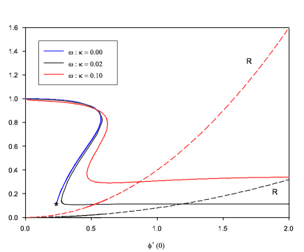
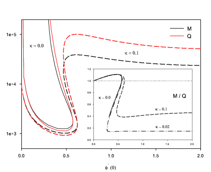
Figure 1: Left: The frequency $\omega$ and the value $R(0)$ as functions of $\phi^{\prime}(0)$ for Q-balls ($\kappa=0$) and boson stars $(\kappa=0.1,\kappa=0.02)$. Right: Mass and charge of the solutions. The ratio $M/Q$ is plotted in the insert.

The Q-balls can be constructed numerically by increasing progressively the control parameter $\phi^{\prime}(0)$, forming a branch to which we refer as the main branch. In the limit $\phi^{\prime}(0)\to 0$, the vacuum configuration $\phi(r)=0$ is uniformly approached while $\omega\to 1$. The convergence is slow and quantities like the mass (and also the charge) converge to a finite value, forming a mass gap. As demonstrated by Fig. 1, the solutions exist up to a maximal value of parameter $\phi^{\prime}(0)$; we find $\phi^{\prime}(0)_{max}\approx 0.572$ corresponding to a frequency $\omega\approx 0.84$. Solving the equations for lower values of the frequency reveals the existence of another branch of Q-balls, let us call it the second branch. We found strong indications that these solutions exist for $\phi^{\prime}(0)\in]\phi^{\prime}(0)_{min},\phi^{\prime}(0)_{max}]$ and $\omega\in]0,0.84[$ (with $\phi^{\prime}(0)_{min}\approx 0.25$). The numerical construction of the solutions of the second branch is difficult for the small values of $\omega$ (the star ’$\star$’ on Fig. 1 represents the limit where our numerical solutions became unreliable). In this region, the profile of the function $\phi(r)$ presents a pronounced abrupt wall for $r\approx R_{w}$ (we define the parameter $R_{w}$ as the value of $r$ where the function $\phi^{\prime}(r)$ attains its local minimum). This wall separates two plateaus; the first one has $\phi(r)\sim 1$ (for $r<R_{w}$) and the second at $\phi=0$ (for $r>R_{w}$). As an illustration of this result the profiles of the two solitons corresponding to $\phi^{\prime}(0)=0.3$ (one for each branch) are shown on Fig. 2. The numerical results show that, in the limit $\phi^{\prime}(0)\to\phi^{\prime}(0)_{min}$, the mass, the charge and the radius $R_{w}$ of the solution tends to infinity: this can be related to the fact that no attractive force (like gravity) is operating, as a consequence the star can spread arbitrarily large in space.

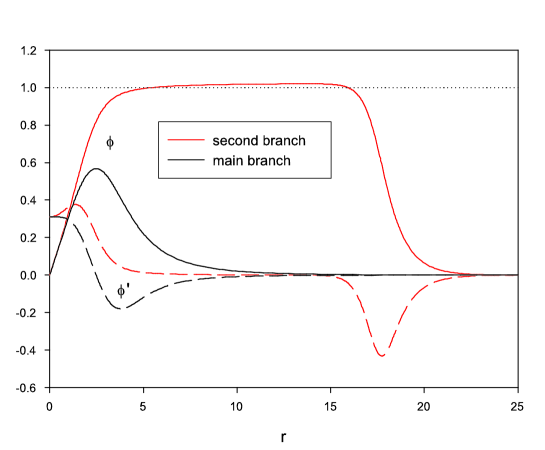
Figure 2: The profiles $\phi$ and $\phi^{\prime}$ for the two Q-balls (one on each branch) corresponding to $\phi^{\prime}(0)=0.3$.

The solutions on the main branch correspond to high frequencies $1>\omega>0.84$ and have $M/Q>1$; interestingly the solutions of second branch correspond to low frequencies ($0.84>\omega>0$) and have $M/Q<1$. Following standard arguments about the classical stability of Q-balls, only the solutions of the second branch are classically stable.

3.2 Boson stars

Boson stars correspond to deformations of the Q-balls (see previous section) for $\kappa>0$. Once coupled to gravity the pattern of the solutions change qualitatively. The major difference between boson stars and Q-balls is that -contrary to Q-balls- boson stars exist for large values of $\phi^{\prime}(0)$. Several features of Q-balls and bosons stars are illustrated on Fig. 1 for three values of $\kappa$.

For fixed $\kappa$ and $\phi^{\prime}(0)$ increasing, the value $b(0)$ approaches zero while the value of the Ricci scalar at the origin (say $R\equiv R(0)$) increases roughly quadratically. This suggests that a singular configuration is approached in the limit $\phi^{\prime}(0)\to\infty$. Outside the central region (we find typically for $r\in[R_{w}/10,\infty]$) the metric and the the scalar field are rather intensive to the increase of $\phi^{\prime}(0)$. In particular, $\omega,M,Q,R_{w}$ approaches constants for $\phi^{\prime}(0)\to\infty$ (these constants depend, off course, on $\kappa$). Note that no counterpart of the second branch of Q-ball is found. This phenomenon can be explained by the fact that the attracting gravitational interaction keeps the matter field relatively compact and does not allow for an extension in an arbitrarily large volume.

Since Q-balls ($\kappa=0$) do not exist for $\phi^{\prime}(0)>\phi^{\prime}(0)_{max}$, it is natural to examine the behavior of boson stars ($\kappa>0$) for fixed values of $\phi^{\prime}(0)$, greater than $\phi^{\prime}(0)_{max}$, and decreasing the parameter $\kappa$. It turns out that the parameters $R_{w}$ (and similarly $M,Q$) increases, likely tending to infinity in the limit $\kappa\to 0$. We find in particular $R_{w}\sim 1/\kappa$: as it could be expected, the decreases gravity, through the effective coupling parameter $\kappa$, allows for compact object with larger and larger size to form.

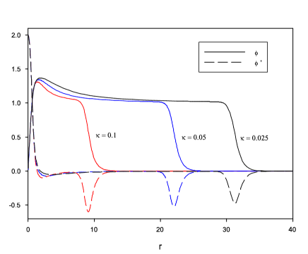
(a) Matter field

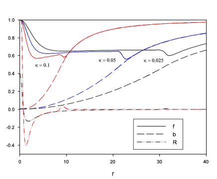
(b) Metric function

Figure 3: Profiles of the scalar and metric functions for $\kappa=0.1,0.05$ and $\kappa=0.025$.

To illustrate this statement, the profiles of the different fields corresponding to $\kappa=0.1,0.05$ and $\kappa=0.025$ are presented on Fig. 3. We further notice that the Ricci scalar $R(r)$ approaches uniformly the null function although the metric potentials keep non trivial profiles.

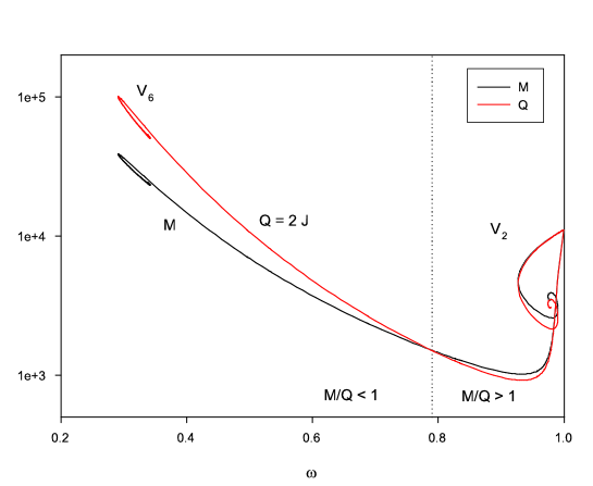
Figure 4: Mass and charge of minimal and self-interacting boson star corresponding to $\kappa=0.1$.

Comparison of the $V_{2}$ and $V_{6}$ potentials : As pointed out already, boson stars exist with the mass potential $V_{2}$. On Fig. 4 the charge and the mass of the minimal and self-interacting boson stars are superposed. The non linear interaction clearly allows for solutions with a lower frequency, then also corresponding to a slower speed of rotation on the horizon. The minimal boson stars have $M/Q>1$ on their whole domain of $w$. Accordingly, they have no positive binging energy and are classically unstable. The interaction makes the solutions classically stable for the low values of the frequency.

3.3 Black holes

The construction of black holes in Einstein gravity and for the mass potential constitutes the object of [6]. It was found that black holes exist in a very specific domain of the parameters $w,r_{H}$ (see in particular Fig. 1 of [6]). Here we will present the influence of the self-interaction $V_{6}$ on the families of black holes obtained in that paper.

The pattern of solutions is quite involved. It turns out that, corresponding to a fixed value of $w$, two (and sometimes even four) branches of black holes exist on specific intervals of the horizon parameter $r_{H}$. In order to describe the pattern, let us choose one particular boson star characterized by a frequency $w$. Integrating the black holes equations for this value of $w$ we find that one branch of black holes exist for $r_{H}\in]0,r_{H,max}]$. In the limit $r_{H}\to 0$ the limiting solution on this branch approaches the starting boson star; correspondingly, the temperature $T_{H}$ diverges while the horizon area $A_{H}$ tends to zero. In the following, we will refer to such a family of black holes as to the BS-branch. The data corresponding to $w=0.995$ (i.e. close to the limiting value $w=1$) is reported on Fig. 5.

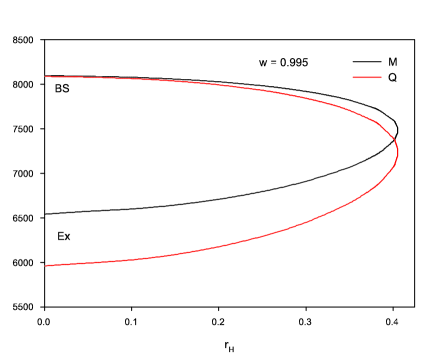
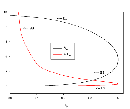
Figure 5: Left: Mass and charge of the black hole for $w=0.995$ and $\kappa=0.1$ as function of the horizon $r_{H}$. Right: Temperature and horizon area as functions of $r_{H}$.

A careful study of the equations for the same value of $w$ reveal that another branch of solutions exists, also labeled by the horizon parameter $r_{H}$. In the limit $r_{H}\to 0$ the solutions of this second branch terminate either into an extremal black hole (in this case the temperature $T_{H}$ tends to zero) or into another boson star with the same $w$. Setting $w=0.995$ (see Fig. 5) the second branch indeed terminates into an extremal black hole; we labeled it the $Ex$-branch. The $Ex$-branch and $BS$-branch coincide for $r_{H}=r_{H,max}$. We found that the value $r_{H,max}$ decreases slowly with $w$; for example $r_{H,max}\approx 0.4$ for $w=0.995$ and $r_{H,max}\approx 0.36$ for $w=0.3$.

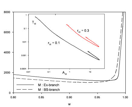
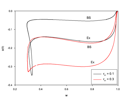
Figure 6: Left: Mass of the boson star (dashed line) and of the extrema solution (solid line) for $\kappa=0.1$ as function $w$ region $w\sim 1$. Insert : Temperature as function of the horizon area for two values of $r_{H}$. Right: Value of the scalar field at the horizon as function of $w$ for two values of $r_{H}$.

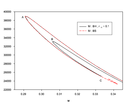
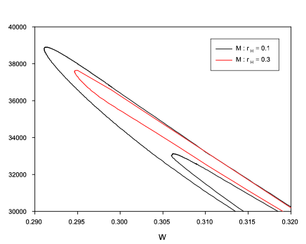
Figure 7: Left: Mass of the black hole (black line) with $r_{H}=0.1$ and $\kappa=0.1$ as function $w$ in the critical region; The mass of the boson star (dashed red). Right: Mass of the black hole with $r_{H}=0.1$ and $r_{H}=0.3$ (for $\kappa=0.1$) as function $w$ in the critical region.

Repeating this operation with different values of $w$ to determine the domain of existence of the solutions is quite demanding; we therefore employed a slightly different strategy. We constructed the families of black holes corresponding to fixed values of $r_{H}$ and varying $w$. Several features of the pattern are illustrated on Figs. 6,LABEL:data_xh_01_b where some parameters (mainly the mass) are reported in function of $w$. These figures, where for definiteness we set $\kappa=0.1$, appeals several comments :

• On Fig.6 (left part) the mass of boson star and of the extremal solution are given in the region $w\sim 1$.

• The values of the scalar field on the horizon for the black holes with $r_{H}=0.1$ and $r_{H}=0.3$ are superposed on right side of Fig. 6. The $A_{H},T_{H}$ relation for these black holes is supplemented in the insert in the left side of the figure.

• For $w>0.97$ and $w<0.35$ we have $M_{BS}>M_{Ex}$. For intermediate values of $w$ we have instead $M_{BS}<M_{Ex}$. This contrasts with the case of the mass term (see [6]).

• Figs. 7 show the mass-frequency dependence in the region of the small frequencies. The left side shows a comparison between the mass of boson star (dashed red line) and the mass of the black hole corresponding to $r_{H}=0.1$ (black line). The curve corresponding to the black holes of the $BS$-branch is all long very close to the curve corrsponding to the boson star. These curves can hardly be distinguished on the graphic but separate only when the boson star mass starts spiraling. For each $w$ such that $w\in[0.307,0.334]$ four black holes with different masses exist. The $BS$-branch and $Ex$-branch join at the point marked $C$ corresponding to $w\approx 0.334$ and $M\approx 25.000$. This value is very close to the mass of the corresponding boson star.

• Increasing the horizon value, the pattern get simpler. In particular the points marked $B,C$ on the figure disappear and only two solutions persist for all accessible values of $w$. The masses corresponding to $r_{H}=0.1$ and $r_{H}=0.3$ are compared on Fig. 7 (right part).

As Figs. LABEL:data_a and LABEL:data_xh_01_b reveal, the pattern of the black holes solutions is quite involved and uneasy to describe solely with the control parameters $r_{H}$ and $w$. On Fig. 8 we illustrate another feature of the solutions by using a mass-temperature plot for the solutions corresponding to $r_{H}=0.1$ and $r_{H}=0.3$. In each case, the points where the curves stop correspond to the limit $w\to 1$. The use of $T_{H}$ as parameter allows one to disentangled the BS and Ex-branches. The range of accessible temperature for a definite $r_{H}$ decreases while $r_{H}$ increases and collapse for $r_{H}\sim 0.4$. The three points labeled $A,B,C$ on this graphic correspond to the critical values marked also in Fig. 7.

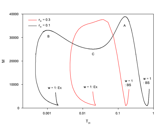
Figure 8: Mass-Temperature relation for black holes with $r_{H}=0.1$ and $r_{H}=0.3$ (here $\kappa=0.1$).

To conclude this section let us stress a few differences between the families of black holes associated with the $V_{2}$ and $V_{6}$ potentials :

• The black holes can exist for smaller values of $w$ (i.e. angular velocity at the horizon) than for the mass potential.

• Our results suggest that considering smaller values of $\kappa$ would result into the occurrence of black holes with arbitrarily small values of $w$. The numerical construction becomes however difficult.

• The black holes with the low values for $w$ have much higher masses (and charge $Q$) than the ones close to the limit $w=1$.

4 Solutions in EGB gravity

As said already, the influence of the Gauss-Bonnet term on spinning boson stars existing in 5-dimensional gravity was studied by several authors. A general feature seems to be that any solution of this type can be deformed continuously by progressively increasing the Gauss-Bonnet parameter $\alpha$ and ceases to exist at a critical value, say $\alpha_{max}$.

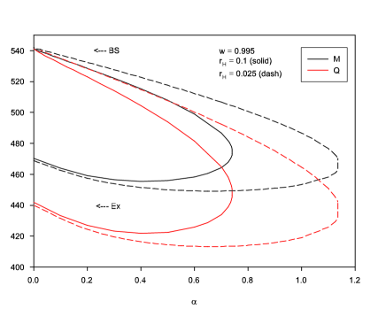
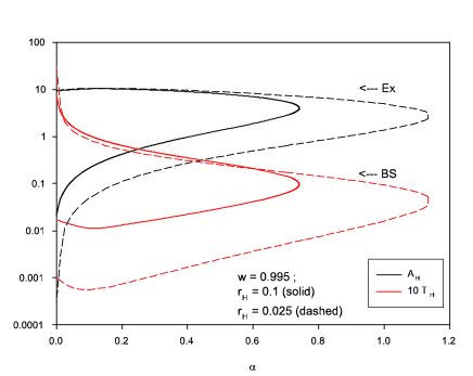
Figure 9: Left: Mass and charge of black holes with $w=0.995$ and $r_{H}=0.1$ (solid) and $r_{H}=0.025$ (dashed) as function $\alpha$. Right: Horizon area and temperature of black holes with $w=0.995$ and $r_{H}=0.1$ (solid) and $r_{H}=0.025$ (dashed) as function $\alpha$.

The reasons of this limitation can be found analytically [10], [12] by performing a Taylor expansion of the solutions around the origin. It turns out that Gauss-Bonnet interaction implies some quadratic constraints like (15) between the Taylor coefficients; as a consequence some coefficients might become complex for large values of $\alpha$ and the solution stops to be real. Since the black holes are only considered outside their event horizon, the question of their existence for $\alpha>0$ raises naturally.

Table 1: Critical value of $\alpha$ for a few values of $w$ and $r_{H}$. The two first lines correspond to the branch with the higher mass and the last line corresponds to the branch with the lower mass.

$\alpha_{max}$	$r_{H}$ = 0.025	$r_{H}$ = 0.1
$w$ = 0.995	1.15	0.7
$w$ = 0.94	0.9	0.26
$w$ = 0.98	0.16	0.02

We have examined the deformations of the black holes for $\alpha>0$. For simplicity, we have considered the case of a mass-potential. As pointed out above there exist two black holes corresponding to a choice of $r_{H}$ and $w$. We distinguish these solution as belonging to the $Ex$-branch (connected to extremal black holes) and $BS$-branch (connected to boson star). It turns out that the deformation of a couple of such solutions for $\alpha>0$ leads to two branches of solutions which terminate into a single solution at some maximal value $\alpha_{max}(w,r_{H})$. On Fig. 9, we show the dependence of the mass $M$ and of the charge $Q$ on $\alpha$ for $w=0.995$ and for two values of $r_{H}$ (for instance $r_{H}=0.025$ and $r_{H}=0.1$). We have constructed the solutions for several values of $w$ and obtaining the same pattern. Values of $\alpha_{max}$ corresponding to a few choices of $w$ and $r_{H}$ are given in Table 1. For a fixed $w$, the value $\alpha_{max}(w,r_{H})$ decreases monotonically with increasing $r_{H}$. We noticed a strong decrease with $\alpha$ of the temperature of the solution corresponding to the $BS$-branch while increasing $\alpha$.

5 Conclusions

Very recently there was a strong interest for astrophysical objects presenting scalar hairs, see for example [23], [24], [25], [26]. This type of research motivate the study of the possible hair structure occurring around compact gravitating objects. In many cases, bosons star and/or hairy black holes are continuously connected to vacuum solutions, i.e. they loose their hair in some limit of the parameter space. In this respect, the hairy black holes constructed in [6] are different since their scalar cloud cannot be dissolved by taking a special limit; in other words they are disjoined from the well know Myers-Perry vacuum solutions. This property is, likely, due to a peculiar non-linear effect in the equations. The question of the persistence of this feature in more general models then raises naturally.

In this paper, we have extended the results of [6] in two directions:

• We included a self-interaction for the scalar field by mean of a potential possessing a non trivial vacuum manifold. We guess that all intermediated potentials between $V_{6}$ and $V_{2}$ would lead to similar properties.

• Extending the gravity sector by a Gauss-Bonnet term which is believed to encode corrections to Einstein gravity coming from string theory.

The results is that the clouds of the solutions keep their distinguished property in both cases. As new features let us stress that the self-interaction allows for spinning black hole with (in principle) arbitrarily small-but non vanishing- angular velocity on the horizon, say $w$. Only when this parameter become sufficiently small do the boson stars constitute classically stable configurations.

In the case of EGB gravity, we have shown that, for all values of $w,r_{H}$ allowing for hairy black holes, there exist a couple of corresponding solutions. These two solutions exist up to a maximal value of the Gauss-Bonnet coupling constant, say $\alpha_{max}$, and converge to a single solution in the limit $\alpha\to\alpha_{max}$.
Note added: While finishing this paper we were aware of [27] where hairy black holes in four dimensional Einstein-Gauss-Bonnet-dilaton gravity are constructed.

References

- [1] C. A. R. Herdeiro and E. Radu, Phys. Rev. Lett. 112, 221101 (2014) [arXiv:1403.2757 [gr-qc]].
- [2] C. Herdeiro and E. Radu, Class. Quant. Grav. 32, no. 14, 144001 (2015) [arXiv:1501.04319 [gr-qc]].
- [3] C. A. R. Herdeiro, E. Radu and H. Runarsson, Phys. Rev. D 92, no. 8, 084059 (2015) [arXiv:1509.02923 [gr-qc]].
- [4] R. C. Myers and M. J. Perry, Ann. Phys. 1972, 304 (1986).
- [5] T. Delsate, J. V. Rocha and R. Santarelli, Phys. Rev. D 89 (2014) 121501 [arXiv:1405.1433 [gr-qc]].
- [6] Y. Brihaye, C. Herdeiro and E. Radu, Phys. Lett. B 739 (2014) 1 [arXiv:1408.5581 [gr-qc]].
- [7] O. J. C. Dias, G. T. Horowitz and J. E. Santos, JHEP 1107 (2011) 115 [arXiv:1105.4167 [hep-th]].
- [8] S. Stotyn, C. D. Leonard, M. Oltean, L. J. Henderson and R. B. Mann, Phys. Rev. D 89 (2014) 4, 044017 [arXiv:1307.8159 [hep-th]].
- [9] S. Stotyn, M. Park, P. McGrath and R. B. Mann, Phys. Rev. D 85 (2012) 044036 [arXiv:1110.2223 [hep-th]].
- [10] L. J. Henderson, R. B. Mann and S. Stotyn, Phys. Rev. D 91 (2015) 2, 024009 [arXiv:1403.1865 [gr-qc]].
- [11] Y. Brihaye and J. Riedel, Phys. Rev. D 89 (2014) 10, 104060 [arXiv:1310.7223 [gr-qc]].
- [12] Y. Brihaye and B. Hartmann, “Minimal boson stars in 5 dimensions: classical instability and existence of ergoregions,” arXiv:1509.04534 [hep-th].
- [13] E. W. Mielke and F. E. Schunck, gr-qc/9801063.
- [14] D. Astefanesei and E. Radu, Nucl. Phys. B 665, 594 (2003) [gr-qc/0309131].
- [15] A. Prikas, Phys. Rev. D 69 (2004) 125008 [hep-th/0404037].
- [16] B. Hartmann, J. Riedel and R. Suciu, Phys. Lett. B 726 (2013) 906 [arXiv:1308.3391 [gr-qc]].
- [17] B. Hartmann, B. Kleihaus, J. Kunz and M. List, Phys. Rev. D 82, 084022 (2010).
- [18] M. S. Volkov and E. Wohnert, Phys. Rev. D 66, 085003 (2002).
- [19] R. Friedberg, T. D. Lee and Y. Pang, Phys. Rev. D 35, 3658 (1987).
- [20] P. Dorey, K. Mersh, T. Romanczukiewicz and Y. Shnir, Phys. Rev. Lett. 107 (2011) 091602 [arXiv:1101.5951 [hep-th]].
- [21] Y. Brihaye, A. Cisterna, B. Hartmann and G. Luchini, “From topological to non-topological solitons: kinks, domain walls and Q-balls in a scalar field model with non-trivial vacuum manifold,” arXiv:1511.02757 [hep-th].
- [22] U. Ascher, J. Christiansen and R. D. Russell, Math. Comput. 33 (1979), 659; ACM Trans. Math. Softw. 7 (1981), 209.
- [23] P. Grandclement, C. Some and E. Gourgoulhon, Phys. Rev. D 90 (2014) 2, 024068 doi:10.1103/PhysRevD.90.024068 [arXiv:1405.4837 [gr-qc]].
- [24] Z. Meliani, F. H. Vincent, P. Grandclement, E. Gourgoulhon, R. Monceau-Baroux and O. Straub, “Circular geodesics and thick tori around rotating boson stars,” arXiv:1510.04191 [astro-ph.HE].
- [25] F. H. Vincent, Z. Meliani, P. Grandclement, E. Gourgoulhon and O. Straub, “Imaging a boson star at the Galactic center,” arXiv:1510.04170 [gr-qc].
- [26] S. Troitsky, “Supermassive dark-matter Q-balls in galactic centers?,” arXiv:1510.07132 [hep-ph].
- [27] B. Kleihaus, J. Kunz, S. Mojica and E. Radu. Spinning black holes in Einstein–Gauss-Bonnet–dilaton theory: non-perturbative solutions arXiv:1511.05513.