Chaotic orbits for systems of nonlocal equations

Abstract.

We consider a system of nonlocal equations driven by a perturbed periodic potential. We construct multibump solutions that connect one integer point to another one in a prescribed way. In particular, heteroclinic, homoclinic and chaotic trajectories are constructed.

This is the first attempt to consider a nonlocal version of this type of dynamical systems in a variational setting and the first result regarding symbolic dynamics in a fractional framework.

1. Introduction

Goal of this paper is to construct heteroclinic and multibumps orbits for a class of systems of integrodifferential equations. The forcing term of the equation comes from a multiwell potential (for simplicity, say periodic and centered at integer points, though more general potential with a discrete set of minima may be similarly taken into account).

The solutions constructed connect the equilibria of the potential in a rather arbitrary way and thus reveal a chaotic behavior of the problem into consideration.

More precisely, the mathematical framework that we consider is the following. Given $s\in\left(\frac{1}{2},1\right)$, we consider an interaction kernel $K:\mathbb{R}\to[0,+\infty]$, satisfying the structural assumptions $K(-x)=K(x)$,

(1.1) $$\frac{\theta_{0}\;(1-s)\;\chi_{[-\rho_{0},\rho_{0}]}(x)}{|x|^{1+2s}}\leqslant K(x)\leqslant\frac{\Theta_{0}\;(1-s)}{|x|^{1+2s}}$$

for some $\rho_{0}\in(0,1]$ and $\Theta_{0}\geqslant\theta_{0}>0$, and

(1.2) $$|\nabla K(x)|\leqslant\frac{\Theta_{1}}{|x|^{2+2s}}$$

for some $\Theta_{1}>0$.

We consider the energy associated to such interaction kernel: namely, for any measurable function $Q:\mathbb{R}\to\mathbb{R}^{n}$, with $n\in\mathbb{N}$, $n\geqslant 1$, we define

(1.3) $$E(Q):=\iint_{\mathbb{R}\times\mathbb{R}}K(x-y)\,\big{|}Q(x)-Q(y)\big{|}^{2}\,dx\,dy.$$

Our goal is to take into account the integrodifferential equation satisfied by the critical points of $E$.

For this, given an interval $J\subseteq\mathbb{R}$, a measurable function $Q:\mathbb{R}\to\mathbb{R}^{n}$, with $E(Q)<+\infty$, and $f\in L^{1}(J,\mathbb{R}^{n})$ we say that $Q$ is a solution of

(1.4) $${\mathcal{L}}(Q)(x)+f(x)=0$$

if

(1.5) $$2\iint_{\mathbb{R}\times\mathbb{R}}K(x-y)\,\big{(}Q(x)-Q(y)\big{)}\cdot\big{(}\psi(x)-\psi(y)\big{)}\,dx\,dy+\int_{\mathbb{R}}f(x)\cdot\psi(x)\,dx=0,$$

for any $\psi\in C^{\infty}_{0}(J,\mathbb{R}^{n})$. We remark that (1.4) provides a single equation for $n=1$ and a system of equations for $n\geqslant 2$.

In the strong version, the operator ${\mathcal{L}}(Q)$ may be interpreted as the integrodifferential operator

$$4\int_{\mathbb{R}}K(x-y)\,(Q(x)-Q(y))\,dy,$$

with the singular integral taken in its principal value sense.

The prototype of the interaction kernel that we have in mind is $K(x):=\frac{1-s}{|x|^{1+2s}}$. In this case, the operator ${\mathcal{L}}(Q)$ in (1.4) is (up to multiplicative constants) the fractional Laplacian $(-\Delta)^{s}Q$.

The setting considered in (1.1) is very general, since it comprises operators which are not necessarily homogeneous or isotropic.

The particular equation that we consider in this paper is

(1.6) $${\mathcal{L}}(Q)(x)+a(x)\,\nabla W(Q(x))=0\qquad{\mbox{ for any }}x\in\mathbb{R}.$$

We suppose that $W\in C^{1,1}(\mathbb{R}^{n})$ and that it is periodic of period $1$, that is $W(\tau+\zeta)=W(\tau)$ for any $\tau\in\mathbb{R}^{n}$ and $\zeta\in\mathbb{Z}^{n}$.

We also assume that the minima of $W$ are attained at the integers: namely we suppose that

(1.7) $$W(\zeta)=0 \zeta\in\mathbb{Z}^{n} W(\tau)>0 \tau\in\mathbb{R}^{n}\setminus\mathbb{Z}^{n}$$ for any  and that  for any .

Also, we suppose that the minima of $W$ are “nondegenerate”. More precisely, we assume that there exist $r\in(0,\,1/4]$, $c_{0}\in(0,1)$ and $C_{0}\in(1,+\infty)$ such that

(1.8) $$c_{0}\,|\tau|^{2}\leqslant W(\tau)\leqslant C_{0}\,|\tau|^{2}\qquad{\mbox{ for any }}\tau\in B_{r}.$$

These assumptions on $W$ are indeed rather general and fit into the well-established theory of multiwell potentials.

The function $a$ can be considered as a perturbation of the potential, and many structural results hold under the basic conditions that $a\in C^{1}(\mathbb{R})$ with $a^{\prime}\in L^{\infty}(\mathbb{R})$, and that there exist $\underline{a}\in(0,1)$ and $\overline{a}\in(1,+\infty)$ such that

(1.9) $$\underline{a}\leqslant a(x)\leqslant\overline{a}\qquad{\mbox{ for any }}x\in\mathbb{R}.$$

On the other hand, to construct unstable orbits, one also assumes that $a$ satisfies a “nondegeneracy condition”. Several general hypotheses on $a$ could be assumed for this scope (see e.g. page 227 in [RCZ00]), but, to make a simple and concrete example, we stick to the case in which

(1.10) $$a(x):=a_{1}+a_{2}\cos(\varepsilon x),$$

with $\varepsilon>0$ to be taken suitably small and $a_{1}>a_{2}>0$ (to be consistent with (1.9) one can take $a_{1}:=(\overline{a}+\underline{a})/2$ and $a_{2}:=(\overline{a}-\underline{a})/2$).

Notice that when $\varepsilon=0$, the perturbation function $a$ reduces to a constant and thus it has no effect on the structure of the solutions of (1.6). On the other hand, we will show that for small $\varepsilon$ the perturbation $a$ produces a variety of geometrically very different solutions. Namely, under the conditions above, we construct solutions of (1.6) which connect chains of integers, thus proving a sort of “chaotic” behavior for this type of solutions (roughly speaking, the sequences of integers can be arbitrarily prescribed in a given class, thus providing a “symbolic dynamics”). The behavior of this chaotic trajectories is depicted in Figure 1.

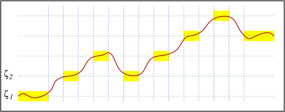
Figure 1. A chaotic trajectory.

More precisely, the main result that we prove in this paper is the following:

Theorem 1.1.

Let $\zeta_{1}\in\mathbb{Z}^{n}$ and $N\in\mathbb{N}$. There exist $\zeta_{2},\dots,\zeta_{N}\in\mathbb{Z}^{n}$ and $b_{1},\dots,b_{2N-2}\in\mathbb{R}$, with $b_{i+1}\geqslant b_{i}+3$ for all $i=1,\dots,2N-3$, and a solution $Q_{*}$ of (1.6) such that

$$\zeta_{i+1}\neq\zeta_{i}{\mbox{ for any }}i\in\{1,\dots,N-1\},$$

$$\lim_{x\to-\infty}Q_{*}(x)=\zeta_{1},$$

$$\sup_{x\in(-\infty,b_{1}]}|Q_{*}(x)-\zeta_{1}|\leqslant\frac{1}{4},$$

$$\sup_{x\in[b_{2i},b_{2i+1}]}|Q_{*}(x)-\zeta_{i+1}|\leqslant\frac{1}{4}\qquad{\mbox{ for all }}i=1,\dots,N-2,$$

$$\sup_{x\in[b_{2N-2},+\infty)}|Q_{*}(x)-\zeta_{N}|\leqslant\frac{1}{4}$$

and $$\lim_{x\to+\infty}Q_{*}(x)=\zeta_{N}.$$

More quantitative versions of Theorem 1.1 will be given in the forthcoming Theorems 9.4 and 10.3.

The result contained in Theorem 1.1 may be seen as the first attempt in the literature to deal with heteroclinic, homoclinic and chaotic orbits for systems of equations driven by fractional operators (as a matter of fact, to the best of our knowledge, Theorem 1.1 is new even in the case of a single equation with the fractional Laplacian).

For local equations, the study of these types of orbits has a long and celebrated tradition and the local counterpart of Theorem 1.1 is a celebrated result in [Rab89] (see also [CZR91, Sér92, Rab94, Rab94, Bes95, Max97, Rab97, BM97, BB98, ABM99, RCZ00, Rab00] and the references therein for important related results).

We point out that the nonlocal character of the equation generates several difficulties in the construction of the connecting orbits, since all the variational methods available in the literature are deeply based on the possibility of “glueing” trajectories to provide admissible competitors. Of course, in the nonlocal case this glueing procedure is more problematic, since the energy is affected by the nonlocal interactions.

In the nonlocal case, as far as we know, multibump solutions have not been studied in the existing literature. In the homogeneous case (i.e. when $a$ is constant), heteroclinic solutions have been constructed in [PSV13, CS15, CP16], but the methods used there do not easily extend to inhomogeneous cases (since sliding methods and extension techniques are taken into account) and cannot lead to the construction of chaotic trajectories. In particular, the reader can compare Theorem 1.1 here with Theorem 1 in [PSV13], Theorem 2.4 in [CS15] or Theorem 1 in [CP16]: all these results provide the existence of transition layers in one dimension for spatially homogeneous doublewell potentials (and in this sense are related to Theorem 1.1 here when $N=2$), but the methods heavily use maximum principle or extension techniques, so they cannot be easily adapted to consider higher dimensional cases and inhomogeneous cases (also, extensions methods cannot be applied for general interaction kernels).

Also, in the framework of the existing literature, this paper is the first attempt to combine the very prolific variational techniques used in dynamical systems to construct special types of orbits with the abundant new tools arising in the study of nonlocal integrodifferential equations.

In this sense, we are also confident that the results of this paper can be stimulating for both the scientific communities in dynamical systems and in partial differential equations and they can trigger new research in this field in the near future.

From the point of view of the applications, for us, one of the main motivations for studying nonlocal variational problems as in (1.6) came from similar equations arising in the study of atom dislocations in crystals and in nonlocal phase transition models, see e.g. [GM06, MP12, GM12, DFV14, DPV15, PV15a, PV15b] and [SV12, PSV13, CS15, CP16].

Important connections between nonlocal diffusion and dynamical systems occur also in several other areas of contemporary research, such as in plasma physics, see e.g. [dCN06].

The rest of the paper is organized as follows. First, in Section 2 – which can of course be easily skipped by the expert reader – we give some heuristic comments on the proof of Theorem 1.1, trying to elucidate the role played by the modulation function $a$ introduced in (1.10).

In Section 3 we collect some simple technical lemmata and in Section 4 we introduce the basic regularity estimates needed for our purposes. Then, in Section 5, we develop the theory of the nonlocal glueing arguments. In a sense, this part contains the many novelties with respect to the classical case, since the classical variational methods fully exploit several glueing arguments that are very sensitive to the local behavior of the energy functional.

The use of the glueing results is effectively implemented in Section 6, which contains the new notion of clean intervals and clean points in this framework. Roughly speaking, in the classical case, having two trajectories that meet allows simple glueing methods to work in order to construct competitors. In our case, to perform the glueing methods, we need to attach the trajectories in an “almost tangent” way, and keeping the trajectories close in Lipschitz norm for a sufficiently large interval. This phenomenon clearly reflects the nonlocal character of the problem and requires the definitions and methods introduced in this section.

In Section 7 we develop the minimization theory for the nonlocal energy under consideration. Differently from the classical case, this part has to join a suitable regularity theory, in order to obtain uniform estimates on the nonlocal terms of the energy.

The stickiness properties of the energy minimizers (i.e., the fact that minimizing orbits stay close to the integer points once they get sufficiently close to them) is then discussed in Section 8. This property is based on the comparison of the energy with suitable competitors and thus it requires the nonlocal glueing arguments introduced in Section 5 and the notion of clean intervals given in Section 6.

Section 9 deals with the construction of heteroclinic orbits: namely, for any integer point, we define the set of admissible integers that can be connected with the first one by a heteroclinic orbit (indeed, we will show that this admissible family contains at least two elements).

In Section 10, we complete the proof of Theorem 1.1 by constructing the desired chaotic orbits.

2. A few comments on the proof of Theorem 1.1 and on the role of the modulation function $a$

The proof of Theorem 1.1 is variational and it can be better understood by thinking first to the case $N=2$, i.e. when only one transition from one integer to another takes place. In this case, one first considers a constrained minimization problem, namely one minimizes the action functional among all the trajectories which are forced to stay sufficiently close to the first integer in $(-\infty,b_{1}]$ and sufficiently close to the second integer in $[b_{2},+\infty)$ (the formal details of this constrained minimization argument will be given in Section 7). The goal is, in the end, to choose $b_{2}>b_{1}$ in a suitable way for which the constrained minimal trajectory does not touch the barrier, hence it is a “free” minimizer and so a solution of the desired equation.

To this aim, the appropriate choice of $b_{1}$ and $b_{2}$ has to take advantage of the small, but not negligible, oscillations of the potential induced by the modulating function $a$ in (1.10). Roughly speaking, the points $b_{1}$ and $b_{2}$ will be chosen sufficiently close to the points in which $a$ takes its maximal value, say at distance close to (a multiple of) the period of $a$, or more generally to the distance between two wells of $a$.

In this way, for a minimal trajectory it is not convenient to put its “transition from one integer to the other” too close to the constraints. Indeed, such transition pays energy in virtue of the potential. So, if the transition occurs too close to $b_{1}$, one can consider the translation of the orbit to the right. Such translated orbit will place the transition in the “lowest well” of the modulating function $a$ and so it will pay less potential energy (the energy coming from particle interaction is on the other hand invariant under translation). In this way, we see that the translated orbit would have less energy than the original one, thus providing a contradiction with the minimality assumption (to facilitate the intuition, one can look at Figure 2).

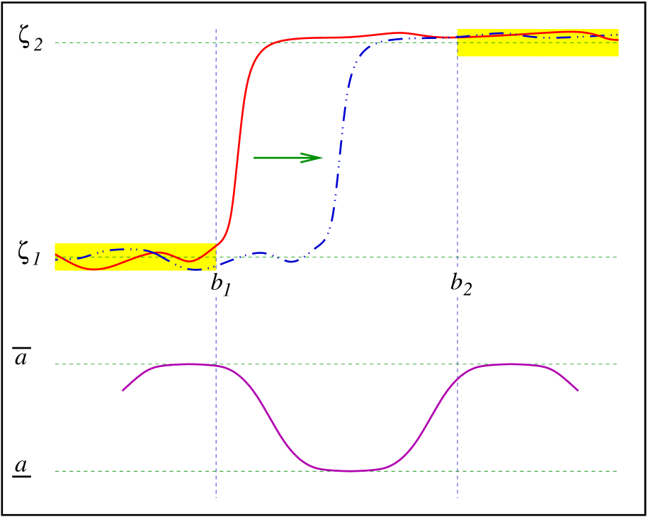
Figure 2. The role of the modulating function $a$ (below), compared with a trajectory with transition too close to $b_{1}$ and its translation (above).

We stress that the nondegeneracy of the function $a$ (that is the fact that $a$ possesses suitable “hills and valleys” in its graph) is indeed crucial in order to perform this variational construction, since it is exactly the ingredient used to allow this energy decreasing under appropriate translations.

Once the transition is set sufficiently far from the constraint, one has to perform suitable cut-and-paste arguments to check that the remaining parts of the trajectory approach the equilibria sufficiently fast, namely the distance from the two limit integers becomes very fast much smaller than the prescription given by the initial constraint and so the trajectory is a true, unconstrained, minimizer.

The choice of $b_{1}$ and $b_{2}$ in terms of the function $a$ will be analytically described in (9.7) and the free minimization procedure is discussed in details in Section 9.

The case in which $N\geqslant 3$, i.e. when multibumps arise, is technically more delicate, since different situations must be taken into account (according to where the touching with the constraint may occur). Also, when $N\geqslant 3$, global translations are not allowed, since they are not compatible with oscillating constraints, and therefore cut-and-paste arguments must be performed together with a local translation procedure. Nevertheless, in spite of these additional difficulties, one may still think that the role of the modulation given by $a$ is to make the transitions near the multiple constraints “too expensive”. For this, once again, one has to place the constraint points $b_{1},\dots,b_{2N-2}$ sufficiently close to the maxima of $a$, so that the transition will have the tendency to occur away from them. The analytic choice of these points will be made in (10.11).

We remark that both the local and the nonlocal case share the variational idea of looking for constrained minimal orbits and then proving that they are in fact unconstrained minimizers – of course, in the nonlocal case the action functional is different than in the local case and it takes into account an interaction energy which is reminiscent of fractional Sobolev spaces. In the nonlocal case, however, the cut-and-paste arguments are more delicate, exactly in view of these interactions coming “from far away”, so they require the “clean point” procedure introduced in Section 6. This procedure is designed exactly in order to make the remote interactions sufficiently small in the glueing methods: roughly speaking, when a glueing procedure makes a sharp angle, the nonlocal energy increases considerably (that is, it is much more than just the sum of the contributions to the left and to the right of the angle). On the other hand, when the function is very flat in a very large neighborhood of the glueing point, this additional energy is rather small, because the values of the function near this point are basically constant and so they give almost no contribution to the interaction energy. An additional energy contribution comes from outside this flatness interval, but, thanks to the decay of the kernel at infinity, it becomes very small as the flatness interval becomes very large.

In this sense, the notation introduced in Section 6 aims to give a precise quantification of the procedure discussed above, also with respect to the energy functional related to Theorem 1.1.

3. Toolbox

This section collects some auxiliary lemmata needed for the proofs of the main theorem. An ancillary tool for these results is the basic theory of the fractional Sobolev spaces. In our setting, given an interval $J\subseteq\mathbb{R}$, we will consider the so-called Gagliardo seminorm of a measurable function $Q:\mathbb{R}\to\mathbb{R}^{n}$, given by

$$[Q]_{H^{s}(J)}:=\left((1-s)\,\iint_{J\times J}\frac{|Q(x)-Q(y)|^{2}}{|x-y|^{1+2s}}\,dx\,dy\right)^{\frac{1}{2}}$$

and the complete fractional norm, given by

$$\|Q\|_{H^{s}(J)}:=[Q]_{H^{s}(J)}+\|Q\|_{L^{2}(J)}.$$

We also denote by $|J|$ the length of the interval $J$. It is useful to observe that $E(Q)$ controls the Gagliardo seminorm, namely, by (1.1),

(3.1) $$\begin{split}{\mbox{ if $|J|\leqslant\rho_{0}$ then }}\qquad E(Q)\;&\geqslant\iint_{J\times J}K(x-y)\,\big{|}Q(x)-Q(y)\big{|}^{2}\,dx\,dy\\ &\geqslant\iint_{J\times J}\frac{\theta_{0}\;(1-s)\;\big{|}Q(x)-Q(y)\big{|}^{2}}{|x-y|^{1+2s}}\,dx\,dy=\theta_{0}\,[Q]_{H^{s}(J)}^{2}\\ {\mbox{ and so }}\qquad\|Q\|_{H^{s}(J)}\;&\leqslant\big{(}\theta_{0}^{-1}E(Q)\big{)}^{\frac{1}{2}}+\|Q\|_{L^{\infty}(J)}.\end{split}$$

In this framework, we recall a Hölder embedding result that is uniform as $s\to 1$:

Lemma 3.1.

Let $s_{0}\in\left(\frac{1}{2},1\right)$ and $s\in[s_{0},1)$. Let $J\subset\mathbb{R}$ be an interval of length $1$. Then, there exists $S_{0}>0$, possibly depending on $n$ and $s_{0}$, such that for any $Q:J\to\mathbb{R}^{n}$ we have that

(3.2) $$[Q]_{C^{0,s-\frac{1}{2}}(J)}\leqslant S_{0}\,[Q]_{H^{s}(J)}.$$

The proof of Lemma 3.1 follows the classical ideas of [Cam63] and can be found essentially in many textbooks. In any case, since we need here to check that the constants are uniform in $s\in[s_{0},1)$ (recall the footnote on page 1) and this detail is often omitted in the existing literature, for completeness we give a selfcontained proof of Lemma 3.1 in Appendix A.

Now we define the energy functional

(3.3) $$I(Q):=E(Q)+\int_{\mathbb{R}}a(x)\,W(Q(x))\,dx,$$

where $E(Q)$ is the “free energy” introduced in (1.3).

In the next result we compute how much the energy charges “long” trajectories:

Lemma 3.2.

Let $\zeta=(\zeta_{1},\dots,\zeta_{n})\in\mathbb{Z}^{n}$, $x_{0}\in\mathbb{R}$ and $Q=(Q_{1},\dots,Q_{n}):\mathbb{R}\to\mathbb{R}^{n}$ be a measurable function such that $Q(x)\in\overline{B_{r}(\zeta)}$ for any $x\leqslant x_{0}$. Assume that $I(Q)<+\infty$ and

(3.4) $$\sup_{x\in\mathbb{R}}|Q_{i}(x)-\zeta_{i}|\geqslant\nu,$$

for some $\nu\in\mathbb{N}$, $\nu\geqslant 1$ and $i\in\{1,\dots,n\}$. Then

$$I(Q)\geqslant E(Q)+2\ell_{Q}\,\underline{a}\,\nu\inf_{{\rm dist}\,(\tau,\;\mathbb{Z}^{n})\geqslant 1/4}W(\tau),$$

where $r$ and $\underline{a}$ are as in (1.8) and (1.9), and

(3.5) $$\ell_{Q}:=\min\left\{\frac{\rho_{0}}{2},\;\left(\frac{1}{4S_{0}\,\big{(}\theta_{0}^{-1}E(Q)\big{)}^{\frac{1}{2}}}\right)^{\frac{2}{2s-1}}\right\}.$$

Proof.

Up to reordering the components of $Q$, we may suppose that $i=1$. Also, by a translation, we may assume that $\zeta=0$.

By (3.1), we find that $[Q]_{H^{s}(J)}\leqslant\big{(}\theta_{0}^{-1}E(Q)\big{)}^{\frac{1}{2}}$, for any interval $J$ with $|J|\leqslant\rho_{0}$. Consequently, by scaling Lemma 3.1, we obtain that $[Q]_{C^{0,s-\frac{1}{2}}(J)}$ is bounded by $S_{0}\,\big{(}\theta_{0}^{-1}E(Q)\big{)}^{\frac{1}{2}}$ for any interval $J$ with $|J|\leqslant\rho_{0}$.

In particular, $|Q_{1}|$ is a continuous curve, which, by (3.4), connects $0$ with $\nu$ and so it passes through all the points of the form $\frac{1}{2}+m$, for any $m\in\{0,\dots,\nu-1\}$. More explicitly, we can say that there exists $X_{m}$ such that $|Q_{1}(X_{m})|=\frac{1}{2}+m$, for all $m\in\{0,\dots,\nu-1\}$. This says that

(3.6) $$Q_{1}(X_{m})\in\frac{1}{2}+\mathbb{Z}.$$

Let now $\ell_{Q}$ be as in (3.5). Then, for any $x\in[X_{m}-\ell_{Q},X_{m}+\ell_{Q}]$,

$$|Q_{1}(x)-Q_{1}(X_{m})|\leqslant S_{0}\,\big{(}\theta_{0}^{-1}E(Q)\big{)}^{\frac{1}{2}}\,\ell_{Q}^{s-\frac{1}{2}}\leqslant\frac{1}{4},$$

and so, by (3.6),

$${\rm dist}\,\big{(}Q_{1}(x),\;\frac{1}{2}+\mathbb{Z}\big{)}\leqslant\frac{1}{4},$$

which gives that

$${\rm dist}\,\big{(}Q_{1}(x),\;\mathbb{Z}\big{)}\geqslant\frac{1}{4}\geqslant r,$$

for any $x\in[X_{m}-\ell_{Q},X_{m}+\ell_{Q}]$. Thus, writing $\tau=(\tau_{1},\dots,\tau_{n})$ and recalling (1.7),

$$W(Q(x))\geqslant\inf_{{\rm dist}\,(\tau_{1},\;\mathbb{Z})\geqslant 1/4}W(\tau),$$

for any $x\in[X_{m}-\ell_{Q},X_{m}+\ell_{Q}]$. As a consequence,

$$\begin{split}I(Q)&\geqslant E(Q)+\sum_{m=0}^{\nu-1}\int_{X_{m}-\ell_{Q}}^{X_{m}+\ell_{Q}}a(x)\,W(Q(x))\,dx\\ &\geqslant E(Q)+2\ell_{Q}\,\underline{a}\,\nu\inf_{{\rm dist}\,(\tau_{1},\;\mathbb{Z})\geqslant 1/4}W(\tau)\\ &\geqslant E(Q)+2\ell_{Q}\,\underline{a}\,\nu\inf_{{\rm dist}\,(\tau,\;\mathbb{Z}^{n})\geqslant 1/4}W(\tau),\end{split}$$

as desired. ∎

4. A bit of regularity theory

Goal of this section is to establish the following regularity result for solutions of (1.6) that are close to an integer in large intervals, with uniform estimates as $s\to 1$:

Lemma 4.1.

Let $s_{0}\in\left(\frac{1}{2},1\right)$ and $s\in[s_{0},1)$.

Let $T>32$, $\rho>0$, $M_{o}>0$, $\zeta\in\mathbb{Z}^{n}$. Let $Q\in L^{\infty}(\mathbb{R},\mathbb{R}^{n})$ be a solution of

$${\mathcal{L}}(Q)(x)+a(x)\nabla W(Q(x))=0$$

in $[-2T,2T]$, with $E(Q)+\|Q\|_{L^{\infty}(\mathbb{R},\mathbb{R}^{n})}\leqslant M_{o}$.

Suppose that

(4.1) $$Q(x)\in\overline{B_{\rho}(\zeta)} x\in[-2T,2T]$$ for any .

Then

$$\|Q\|_{C^{0,1}([-T/16,T/16])}\leqslant\frac{CM_{o}\,(1-s)}{T^{2s}}+C\rho,$$

with $C>0$ depending on $n$, $s_{0}$ and on the structural constants of the kernel and the potential.

Proof.

Up to a translation, we assume that $\zeta=0$, hence (4.1) becomes

(4.2) $$|Q(x)|\leqslant\rho x\in[-2T,2T]$$ for any .

We let $\tau_{o}\in C^{\infty}_{0}([-1,1],[0,1])$ be such that $\tau_{o}(x)=1$ for any $x\in\left[-\frac{1}{2},\frac{1}{2}\right]$. We define $\tau(x):=\tau_{o}(x/T)$ and $u(x):=\tau(x)\,Q(x)$. Notice that, by (4.2),

(4.3) $$|u(x)|\leqslant\rho x\in\mathbb{R}$$ for any .

By Lemma 3.1, we already know that $Q$ is continuous and so it is also a viscosity solution. Therefore (see e.g. formula (2.11) in [BPSV14]), we have that, in the viscosity sense,

(4.4) $$\begin{split}{\mathcal{L}}(u)\;&=\tau\,{\mathcal{L}}(Q)+Q\,{\mathcal{L}}(\tau)-B(Q,\tau)\\ &=-\tau\,a\,\nabla W(Q)+Q\,{\mathcal{L}}(\tau)-B(Q,\tau)\end{split}$$

in $[-T,T]$, where

$$B(Q,\tau)(x):=\int_{\mathbb{R}}K(x-y)\,\big{(}Q(x)-Q(y)\big{)}\big{(}\tau(x)-\tau(y)\big{)}\,dy.$$

We use (1.1) and we notice that, for any $x\in\left[-\frac{T}{4},\frac{T}{4}\right]$,

(4.5) $$\begin{split}|B(Q,\tau)(x)|\;&=\left|\int_{\mathbb{R}\setminus[-T/2,T/2]}K(x-y)\,\big{(}Q(x)-Q(y)\big{)}\big{(}\tau(x)-\tau(y)\big{)}\,dy\right|\\ &\leqslant 2M_{o}\,\Theta_{0}\,(1-s)\,\int_{\mathbb{R}\setminus[-T/2,T/2]}\frac{\big{|}\tau(x)-\tau(y)\big{|}}{|x-y|^{1+2s}}\,dy\\ &=\frac{2M_{o}\,\Theta_{0}\,(1-s)}{T^{2s}}\,\int_{\mathbb{R}\setminus[-1/2,1/2]}\frac{\big{|}\tau_{o}(T^{-1}x)-\tau_{o}(y)\big{|}}{|T^{-1}x-y|^{1+2s}}\,dy\\ &\leqslant\frac{CM_{o}\,\Theta_{0}\,(1-s)}{T^{2s}},\end{split}$$

for some $C>0$.

Furthermore

$$\int_{\mathbb{R}}\frac{|\tau(x+y)+\tau(x-y)-2\tau(x)|}{|y|^{1+2s}}\,dy$$

$$\qquad=\frac{1}{T^{2s}}\int_{\mathbb{R}}\frac{|\tau_{o}(T^{-1}x+y)+\tau_{o}(T^{-1}x-y)-2\tau_{o}(T^{-1}x)|}{|y|^{1+2s}}\,dy\leqslant\frac{C}{T^{2s}}$$

hence

(4.6) $$|Q\,{\mathcal{L}}(\tau)|\leqslant\frac{CM_{o}\,\Theta_{0}\,(1-s)}{T^{2s}},$$

up to renaming $C>0$.

Also, we observe that $\nabla W$ vanishes in $\mathbb{Z}^{n}$, thanks to (1.7). Thus, if we use (1.8), (1.9) and (4.2), we see that if $x\in[-2T,2T]$

(4.7) $$\big{|}\tau(x)\,a(x)\,\nabla W(Q(x))\big{|}\leqslant\overline{a}\big{|}\nabla W(Q(x))-\nabla W(0)\big{|}\leqslant\overline{a}\,\|W\|_{C^{1,1}(\mathbb{R}^{n})}\,|Q(x)|\leqslant C\rho,$$

up to renaming $C$.

So we define

$$f:=-\tau\,a\,\nabla W(Q)+Q\,{\mathcal{L}}(\tau)-B(Q,\tau)$$

and we deduce from (4.5), (4.6) and (4.7) that

(4.8) $$\|f\|_{L^{\infty}([-T/4,T/4],\mathbb{R}^{n})}\leqslant\frac{CM_{o}\,\Theta_{0}\,(1-s)}{T^{2s}}+C\rho,$$

up to renaming $C$. In addition, by (4.4), we know that

(4.9) $${\mathcal{L}}(u)=f$$

in the sense of viscosity. So, we consider any interval $J$ of length $1$ contained in $\left[-\frac{T}{8},\frac{T}{8}\right]$, and we denote by $J^{\prime}$ the dilation of $J$ by a factor $1/2$ with respect to the center of the interval. Thanks to (1.1) and (1.2), we can use Theorem 61 of [CS11] for the equation in (4.9) and obtain that

$$\|u\|_{C^{0,1}(J^{\prime})}\leqslant C\,\big{(}\|u\|_{L^{\infty}(\mathbb{R},\mathbb{R}^{n})}+\|f\|_{L^{\infty}(J,\mathbb{R}^{n})}\big{)}.$$

From this, (4.3) and (4.8), we obtain

$$\|u\|_{C^{0,1}(J^{\prime})}\leqslant\frac{CM_{o}\,\Theta_{0}\,(1-s)}{T^{2s}}+C\rho,$$

up to renaming constants, which gives the desired result. ∎

5. Nonlocal glueing arguments

In the classical case, it is rather standard to glue Sobolev functions that meet at a point. In the fractional setting this operation is more complicated, since the nonlocal interactions may increase the energy of the resulting functions. We will provide in the forthcoming Proposition 5.3 a suitable result which will allow us to use glueing methods.

As a technical point, we remark that we will obtain in these computations very explicit constants (in particular, we check the independence of the constants from $s$ as $s$ is close to $1$).

We first recall a detailed integrability result of classical flavor (with technical and conceptual differences in our cases; similar results in a more classical framework can be found, for instance, in Chapter 3 of [McL00]):

Lemma 5.1.

Let $\beta\in(0,+\infty)$. Let $Q:[0,+\infty)\to\mathbb{R}^{n}$ be a measurable function such that

$$[Q]_{H^{s}([0,1))}<+\infty\;{\mbox{ and }}\;Q(0)=0.$$

Then

(5.1) $$\begin{split}&\int_{0}^{+\infty}x^{-2s}\,|Q(x)|^{2}\,dx\\ &\qquad\leqslant C_{s}\,\left[\,\int_{0}^{\beta}\left[\int_{0}^{x}\frac{|Q(x)-Q(y)|^{2}}{|x-y|^{1+2s}}\,dy\right]\,dx+\frac{2\|Q\|_{L^{\infty}((0,+\infty),\mathbb{R}^{n})}}{(2s-1)\,\beta^{2s-1}}\right],\end{split}$$

where

(5.2) $$C_{s}:=2\left(1+\frac{4}{(2s-1)^{2}}\right).$$

For the facility of the reader, we give the proof of Lemma 5.1 in Appendix B.

Remark 5.2.

If one formally takes $\beta=+\infty$ in Lemma 5.1, then (5.1) reads simply

$$(1-s)\,\int_{0}^{+\infty}x^{-2s}\,|Q(x)|^{2}\,dx\leqslant C_{s}\,[Q]_{H^{s}([0,+\infty)}^{2}.$$

Following is the nonlocal glueing result which fits for our purposes:

Proposition 5.3.

Let $T_{1}\in\mathbb{R}\cup\{-\infty\}$ and $T_{2}\in(T_{1},+\infty]$. Let $x_{0}\in(T_{1},T_{2})$ and

$$\beta\in\big{(}0,\;\min\{T_{2}-x_{0},\;x_{0}-T_{1}\}\big{]}.$$

Let $L:(T_{1},x_{0}]\to\mathbb{R}^{n}$ and $R:[x_{0},T_{2})\to\mathbb{R}^{n}$ be measurable functions with

(5.3) $$\begin{split}&\iint_{(T_{1},x_{0})^{2}}K(x-y)\,|L(x)-L(y)|^{2}\,dx\,dy<+\infty\\ {\mbox{and }}\;&\iint_{(x_{0},T_{2})^{2}}K(x-y)\,|R(x)-R(y)|^{2}\,dx\,dy<+\infty.\end{split}$$

Assume that $L(x_{0})=R(x_{0})$, and let

$$V(x):=\left\{\begin{matrix}L(x)&{\mbox{ if }}x\in(T_{1},x_{0}],\\ R(x)&{\mbox{ if }}x\in(x_{0},T_{2}).\end{matrix}\right.$$

Then

(5.4) $$\begin{split}&\iint_{(T_{1},T_{2})^{2}}K(x-y)\,|V(x)-V(y)|^{2}\,dx\,dy\\ \leqslant\;&\iint_{(T_{1},x_{0})^{2}}K(x-y)\,|L(x)-L(y)|^{2}\,dx\,dy+\iint_{(x_{0},T_{2})^{2}}K(x-y)\,|R(x)-R(y)|^{2}\,dx\,dy\\ +\;&\tilde{C}_{s}\,(1-s)\,\left[\int_{x_{0}-\beta}^{x_{0}}\left(\int_{x}^{x_{0}}\frac{|L(x)-L(y)|^{2}}{|x-y|^{1+2s}}\,dy\right)\,dx+\int_{x_{0}}^{x_{0}+\beta}\left(\int_{x_{0}}^{x}\frac{|R(x)-R(y)|^{2}}{|x-y|^{1+2s}}\,dy\right)\,dx\right]\\ +\;&\frac{\hat{C}_{s}\,(1-s)}{\beta^{2s-1}}\,\Big{[}\|L\|_{L^{\infty}((T_{1},x_{0}),\mathbb{R}^{n})}+\|R\|_{L^{\infty}((x_{0},T_{2}),\mathbb{R}^{n})}\Big{]},\end{split}$$

where

$$\tilde{C}_{s}:=\frac{2\Theta_{0}\,C_{s}}{s}\;{\mbox{ and }}\;\hat{C}_{s}:=\frac{4\,\Theta_{0}\,C_{s}}{s\,(2s-1)},$$

and $C_{s}$ is given in (5.2).

Remark 5.4.

In the spirit of Remark 5.2, we observe that if one takes $K(x):=\frac{1-s}{|x|^{1+2s}}$, then one can formally take $\theta_{0}=\Theta_{0}=1$ and $\beta=+\infty$, and also $T_{1}=-\infty$ and $T_{2}=+\infty$, hence (5.4) reduces to

(5.5) $$[V]_{H^{s}(\mathbb{R})}^{2}\leqslant(1+\tilde{C}_{s})\,\Big{(}[L]_{H^{s}((-\infty,x_{0}))}^{2}+[R]_{H^{s}((x_{0},+\infty))}^{2}\Big{)},$$

with

$$\tilde{C}_{s}=\frac{4}{s}\,\left(1+\frac{4}{(2s-1)^{2}}\right).$$

We stress that formula (5.4) is more complicated, but more precise, than (5.5): for instance, if one sends $s\to 1$ in (5.4) for a fixed $\beta>0$ and then sends $\beta\to 0$, one recovers the classical Sobolev case of functions in $H^{1}((T_{1},T_{2}))$, namely that

(5.6) $$[V]_{H^{1}((T_{1},T_{2}))}^{2}\leqslant[L]_{H^{1}((T_{1},x_{0}))}^{2}+[R]_{H^{1}((x_{0},T_{2}))}^{2}.$$

On the other hand, formula (5.5) in itself cannot recover (5.6), since it looses a constant.

In our framework, the possibility of having good control on the constants plays an important role, for example, in the proof of the forthcoming Proposition 8.1.

Proof of Proposition 5.3.

Up to a translation, we assume that $x_{0}=0$ and $L(x_{0})=R(x_{0})=0$. We also denote $D^{+}:=(0,T_{2})$ and $D^{-}:=(T_{1},0)$. If $T_{1}\neq-\infty$, we notice that $L(T_{1})$ may be defined by uniform continuity, thanks to (5.3) and Lemma 3.1. Thus, we can extend $L(x):=L(T_{1})$ for any $x\leqslant T_{1}$. Similarly, if $T_{2}\neq+\infty$, we extend $R(x):=R(T_{2})$ for any $x>T_{2}$. In this way, by Lemma 5.1,

$$\int_{D^{-}}|x|^{-2s}\,|L(x)|^{2}\,dx$$

$$\qquad\leqslant C_{s}\,\left[\,\iint_{(-\beta,0)\times(x,0)}\frac{|L(x)-L(y)|^{2}}{|x-y|^{1+2s}}\,dx\,dy+\frac{2\|L\|_{L^{\infty}(D^{-},\mathbb{R}^{n})}}{(2s-1)\,\beta^{2s-1}}\right]$$

and $$\int_{D^{+}}|x|^{-2s}\,|R(x)|^{2}\,dx$$

$$\qquad\leqslant C_{s}\,\left[\iint_{(0,\beta)\times(0,x)}\frac{|R(x)-R(y)|^{2}}{|x-y|^{1+2s}}\,dx\,dy+\frac{2\|R\|_{L^{\infty}(D^{+},\mathbb{R}^{n})}}{(2s-1)\,\beta^{2s-1}}\right],$$

where $C_{s}$ is given in (5.2). Therefore, decomposing $(T_{1},T_{2})$ into the two intervals $D^{-}$ and $D^{+}$, and recalling (1.1),

$$\iint_{(T_{1},T_{2})^{2}}K(x-y)\,|V(x)-V(y)|^{2}\,dx\,dy$$

$$\quad-\iint_{(D^{-})^{2}}K(x-y)\,|L(x)-L(y)|^{2}\,dx\,dy-\iint_{(D^{+})^{2}}K(x-y)\,|R(x)-R(y)|^{2}\,dx\,dy$$

$$= 2\iint_{D^{-}\times D^{+}}K(x-y)\,|L(x)-R(y)|^{2}\,dx\,dy$$

$$\leqslant 4\iint_{D^{-}\times D^{+}}K(x-y)\,\Big{(}|L(x)|^{2}+|R(y)|^{2}\Big{)}\,dx\,dy$$

$$\leqslant 4\,\Theta_{0}\,(1-s)\iint_{D^{-}\times D^{+}}\frac{|L(x)|^{2}+|R(y)|^{2}}{|x-y|^{1+2s}}\,dx\,dy$$

$$\leqslant \frac{4\,\Theta_{0}\,(1-s)}{2s}\left[\int_{D^{-}}|x|^{-2s}|L(x)|^{2}\,dx+\int_{D^{+}}|y|^{-2s}|R(y)|^{2}\,dy\right]$$

$$\leqslant \frac{2\,\Theta_{0}\,(1-s)\;C_{s}}{s}\,\left[\iint_{(-\beta,0)\times(x,0)}\frac{|L(x)-L(y)|^{2}}{|x-y|^{1+2s}}\,dx\,dy\right.$$

$$+\left.\iint_{(0,\beta)\times(0,x)}\frac{|R(x)-R(y)|^{2}}{|x-y|^{1+2s}}\,dx\,dy+\frac{2\,\|L\|_{L^{\infty}(D^{-},\mathbb{R}^{n})}}{(2s-1)\,\beta^{2s-1}}+\frac{2\,\|R\|_{L^{\infty}(D^{+},\mathbb{R}^{n})}}{(2s-1)\,\beta^{2s-1}}\right]$$

as desired. ∎

6. A notion of clean intervals and clean points

In the classical case, a standard tool consists in glueing together orbits or linear functions. Due to the analysis performed in Section 5, we see that the situation in the nonlocal case is rather different, since the terms “coming from infinity” can produce (and do produce, in general) a nontrivial contribution to the energy.

To overcome this difficulty, we will need to modify the classical variational tools concerning the glueing of different orbits and of orbits and linear functions. Namely, in our case, we will always perform this glueing at some “clean points” that not only produces values of the functions involved close to the integers, but also that maintains the function close to the integer value in a suitably large interval. This will allow us to use the regularity theory in Section 4 to see that the glueing occurs with “almost horizontal” tangent in a large interval and, consequently, to bound uniformly the nonlocal contributions arising from the nonlocal glueing procedure discussed in Section 5.

Of course, this part is structurally very different from the classical case and, to this end, we introduce some new terminology.

Definition 6.1.

Given $\rho>0$ and $Q:\mathbb{R}\to\mathbb{R}^{n}$, we say that an interval $J\subseteq\mathbb{R}$ is a “clean interval” for $(\rho,Q)$ if $|J|\geqslant|\log\rho|$ and there exists $\zeta\in\mathbb{Z}^{n}$ such that

$$\sup_{x\in J}|Q(x)-\zeta|\leqslant\rho.$$

Of course, the choice of scaling logarithmically the horizontal length of the interval with respect to the vertical oscillations in Definition 6.1 is for further computational convenience, and other choices are also possible (the convenience of this logarithmic choice will be explained in details in the forthcoming Remark 7.4).

Definition 6.2.

If $J$ is a bounded clean interval for $(\rho,Q)$, the center of $J$ is called a “clean point” for $(\rho,Q)$.

Any sufficiently long interval contains a clean interval, and thus a clean point, according to the following result:

Lemma 6.3.

Let $c_{0}$ and $r$ be as in (1.8). Let $\underline{a}$ be as in (1.9) and let $J\subseteq\mathbb{R}$ be an interval. Let $Q:\mathbb{R}\to\mathbb{R}^{n}$, with $I(Q)\in(0,+\infty)$. Let $\rho\in(0,r]$ with

(6.1) $$\left(\frac{\rho}{2S_{0}\,\sqrt{\theta_{0}^{-1}\,E(Q)}}\right)^{\frac{2}{2s-1}}\leqslant|\log\rho|.$$

Suppose that

(6.2) $$|J|\geqslant\frac{\big{[}1+6\,\big{(}2S_{0}\big{)}^{\frac{2}{2s-1}}\big{(}I(Q)\big{)}^{\frac{2s}{2s-1}}\big{]}\,|\log\rho|}{c_{0}\,\underline{a}\,\theta_{0}^{\frac{1}{2s-1}}\,\rho^{\frac{4s}{2s-1}}}.$$

Then there exists a clean interval for $(\rho,Q)$ that is contained in $J$.

Proof.

Assume, by contradiction, that

(6.3) $$J$$ does not contain any clean subinterval.

By (6.2), the interval $J$ contains $N$ disjoint subintervals, say $J_{1},\dots,J_{N}$, each of length $|\log\rho|$, with

(6.4) $$N\geqslant\frac{5\,\big{(}2S_{0}\big{)}^{\frac{2}{2s-1}}\big{(}I(Q)\big{)}^{\frac{2s}{2s-1}}}{c_{0}\,\underline{a}\,\theta_{0}^{\frac{1}{2s-1}}\,\rho^{\frac{4s}{2s-1}}}.$$

By (6.3), none of the subintervals $J_{i}$ is clean. Hence, for any $i\in\{1,\dots,N\}$, there exists $p_{i}\in J_{i}$ such that $Q(p_{i})$ stays at distance larger than $\rho$ from the integer points. Now, letting

$$\ell_{\rho}:=\left(\frac{\rho}{2S_{0}\,\sqrt{\theta_{0}^{-1}\,E(Q)}}\right)^{\frac{2}{2s-1}}$$

and recalling Lemma 3.1, we have that, for any $x\in J^{\prime}_{i}:=[p_{i}-\ell_{\rho},p_{i}+\ell_{\rho}]$,

$$|Q(x)-Q(p_{i})|\leqslant[Q]_{C^{0,s-\frac{1}{2}}(J_{i})}|x-p_{i}|^{s-\frac{1}{2}}\leqslant S_{0}\,\sqrt{\theta_{0}^{-1}\,E(Q)}\,\ell_{\rho}^{s-\frac{1}{2}}=\frac{\rho}{2}.$$

Accordingly, $Q(x)$ stays at distance larger than $\frac{\rho}{2}$ from the integer points, for any $x\in J^{\prime}_{i}$, and so, by (1.8),

$$W(Q(x))\geqslant\frac{c_{0}\,\rho^{2}}{4}.$$

Also, by (6.1), at least half of the interval $J^{\prime}_{i}$ lies in $J_{i}$, hence

$$\int_{J_{i}\cap J_{i}^{\prime}}W(Q(x))\,dx\geqslant\frac{c_{0}\,\rho^{2}\,\ell_{\rho}}{4}.$$

Summing up over $i=1,\dots,N$, and using that the intervals $J_{i}$ are disjoint, we find that

$$I(Q)\geqslant\frac{c_{0}\,\underline{a}\,\rho^{2}\,\ell_{\rho}\,N}{4}.$$

This is a contradiction with (6.4) and so it proves the desired result. ∎

Remark 6.4.

In our applications, we will make use of Lemma 6.3 to orbits whose energy is bounded uniformly. In this way, condition (6.1) simply requires $\rho$ to be small enough and (6.2) reads

$$|J|\geqslant\frac{C_{*}\,|\log\rho|}{\rho^{\frac{4s}{2s-1}}},$$

for some $C_{*}>0$.

7. Minimization arguments

In this section, we introduce the variational problem that we use in the proof of the main results and we discuss the basic properties of the minimizers.

For this, we fix $N\in\mathbb{N}$, $N\geqslant 2$, and we fix $\zeta_{1},\dots,\zeta_{N}\in\mathbb{Z}^{n}$ and $b_{1},\dots,b_{2N-2}\in\mathbb{R}$. We assume that $b_{i+1}\geqslant b_{i}+3$ for any $i\in\{1,\dots,2N-3\}$.

We will use the short notation $\vec{\zeta}:=(\zeta_{1},\dots,\zeta_{N})\in\mathbb{Z}^{nN}$ and $\vec{b}:=(b_{1},\dots,b_{2N-2})\in\mathbb{R}^{2N-2}$. Given $r$ as in (1.8), we also set

(7.1) $$\begin{split}\Gamma(\vec{\zeta},\vec{b}):=\;&\Big{\{}Q:\mathbb{R}\to\mathbb{R}^{n}{\mbox{ s.t. $Q$ is measurable,}}\\ &\qquad{\mbox{ $Q(x)\in\overline{B_{r}(\zeta_{1})}$ for a.e. $x\in(-\infty,b_{1}]$,}}\\ &\qquad{\mbox{ $Q(x)\in\overline{B_{r}(\zeta_{i})}$ for a.e. $x\in[b_{2i-2},b_{2i-1}]$ and\leavevmode\nobreak\ $i\in\{2,\dots,N-1\}$,}}\\ &\qquad{\mbox{ $Q(x)\in\overline{B_{r}(\zeta_{N})}$ for a.e. $x\in[b_{2N-2},+\infty)$}}\Big{\}}.\end{split}$$

Roughly speaking, the set $\Gamma(\vec{\zeta},\vec{b})$ contains all the admissible trajectories that link any integer point in the array $\vec{\zeta}$ to the subsequent one, up to an error smaller than $r$, and using the array $\vec{b}$ to construct appropriate constrain windows, see Figure 3.

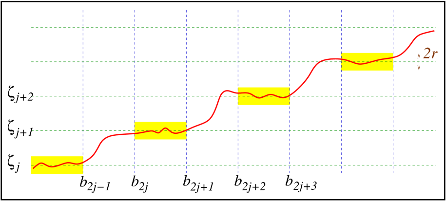
Figure 3. The sets of admissible competitors in $\Gamma(\vec{\zeta},\vec{b})$.

We also define

$$M:=\sum_{j=1}^{N-1}|\zeta_{j+1}-\zeta_{j}|.$$

In this framework, we can consider the minimization problem of the energy functional introduced in (3.3), according to the following result:

Lemma 7.1.

Let $s_{0}\in\left(\frac{1}{2},1\right)$ and $s\in[s_{0},1)$. There exists $Q_{*}\in\Gamma(\vec{\zeta},\vec{b})$ such that

(7.2) $$\sup_{x\in\mathbb{R}}|Q_{*}(x)-\zeta_{1}|\leqslant C,$$

(7.3) $$I(Q_{*})\leqslant C,$$

(7.4) $$[Q_{*}]_{H^{s}(J)}\leqslant C J |J|\leqslant\rho_{0}$$, for any interval  with ,

(7.5) $$\|Q_{*}-\zeta_{1}\|_{C^{0,s-\frac{1}{2}}(\mathbb{R})}\leqslant C,$$

for some $C>0$ possibly depending on $n$, $s_{0}$, $M$ and the structural constants of the kernel and the potential, and

(7.6) $$I(Q_{*})\leqslant I(Q) Q\in\Gamma(\vec{\zeta},\vec{b})$$ for any .

In addition,

(7.7) $$\lim_{x\to-\infty}Q_{*}(x)=\zeta_{1}\;{\mbox{ and }}\;\lim_{x\to+\infty}Q_{*}(x)=\zeta_{N}.$$

Proof.

Let $\mu\in C^{\infty}(\mathbb{R},\,[0,1/2])$ be such that $\mu(0)=1/2$ and $\mu(x)=0$ if $|x|\geqslant 1$. Notice that

$$[1-\mu]_{H^{s}(\mathbb{R})}=[\mu]_{H^{s}(\mathbb{R})}<+\infty.$$

Let

$$\eta(x):=\left\{\begin{matrix}\mu(x)&{\mbox{ if }}x\leqslant 0,\\ 1-\mu(x)&{\mbox{ if }}x>0.\end{matrix}\right.$$

Notice that $\eta(x)=0$ if $x\leqslant-1$ and $\eta(x)=1$ if $x\geqslant 1$. Also, by (5.5),

$$[\eta]_{H^{s}(\mathbb{R})}^{2}\leqslant(1+\tilde{C}_{s})\,\Big{(}[\mu]_{H^{s}(\mathbb{R})}^{2}+[1-\mu]_{H^{s}(\mathbb{R})}^{2}\Big{)}=2(1+\tilde{C}_{s})\,[\mu]_{H^{s}(\mathbb{R})}^{2}=:(C^{\prime}_{s})^{2}.$$

Let also

$$\beta_{i}:=\frac{b_{2i-1}+b_{2i}}{2}\qquad{\mbox{ for any }}i\in\{1,\dots,N-1\}$$

and

$$Q_{0}(x):=\zeta_{1}+\sum_{j=1}^{N-1}(\zeta_{j+1}-\zeta_{j})\,\eta(x-\beta_{j}).$$

Notice that $\beta_{i}$ is an increasing sequence. We also claim that

(7.8) $$Q_{0}\in\Gamma(\vec{\zeta},\vec{b}).$$

To prove this we note that:

• if $x\leqslant b_{1}$ then

  $$x-\beta_{j}\leqslant b_{1}-\beta_{1}=-\frac{b_{2}-b_{1}}{2}\leqslant-\frac{3}{2}$$

  for all $j\in\{1,\dots,N-1\}$, thus $\eta(x-\beta_{j})=0$ for all $j\in\{1,\dots,N-1\}$, and then $Q_{0}(x)=\zeta_{1}$;

• if $i\in\{2,\dots,N-1\}$ and $x\in[b_{2i-2},b_{2i-1}]$, then, for all $j\in\{1,\dots,i-1\}$ we have that

  $$x-\beta_{j}\geqslant b_{2i-2}-\beta_{i-1}=\frac{b_{2i-2}-b_{2i-3}}{2}\geqslant\frac{3}{2},$$

  and thus $\eta(x-\beta_{j})=1$ for all $j\in\{1,\dots,i-1\}$, while for all $j\in\{i,\dots,N-1\}$ we have that

  $$x-\beta_{j}\leqslant b_{2i-1}-\beta_{i}=-\frac{b_{2i}-b_{2i-1}}{2}\leqslant-\frac{3}{2},$$

  and thus $\eta(x-\beta_{j})=0$ for all $j\in\{i,\dots,N-1\}$, therefore a telescopic sum gives that

  $$Q_{0}(x)=\zeta_{1}+\sum_{j=1}^{i-1}(\zeta_{j+1}-\zeta_{j})=\zeta_{1}+(\zeta_{i}-\zeta_{1})=\zeta_{i};$$

• if $x\geqslant b_{2N-2}$ then

  $$x-\beta_{j}\geqslant b_{2N-2}-\beta_{N-1}=\frac{b_{2N-2}-b_{2N-3}}{2}\geqslant\frac{3}{2}$$

  for all $j\in\{1,\dots,N-1\}$, thus $\eta(x-\beta_{j})=1$ for all $j\in\{1,\dots,N-1\}$, and then a telescopic sum gives that

  $$Q_{0}(x)=\zeta_{1}+\sum_{j=1}^{N-1}(\zeta_{j+1}-\zeta_{j})=\zeta_{1}+(\zeta_{N}-\zeta_{1})=\zeta_{N}.$$

These considerations prove (7.8).

Moreover,

$$[Q_{0}]_{H^{s}(\mathbb{R})}\leqslant\sum_{j=1}^{N-1}|\zeta_{j+1}-\zeta_{j}|\,[\eta]_{H^{s}(\mathbb{R})}\leqslant C^{\prime}_{s}\sum_{j=1}^{N-1}|\zeta_{j+1}-\zeta_{j}|.$$

This and (1.1) give that

$$E(Q)\leqslant\Theta_{0}\,[Q_{0}]_{H^{s}(\mathbb{R})}^{2}\leqslant C^{\prime}_{s}\Theta_{0}\,\sum_{j=1}^{N-1}|\zeta_{j+1}-\zeta_{j}|.$$

Also, we have that $\eta(x-\beta_{j})$ takes integer values outside $[\beta_{j}-1,\beta_{j}+1]$ and therefore

$$\int_{\mathbb{R}}a(x)\,W(Q_{0}(x))\,dx\leqslant\overline{a}\sum_{j=1}^{N-1}\int_{\beta_{j}-1}^{\beta_{j}+1}W(Q_{0}(x))\,dx\leqslant 2N\overline{a}\,\sup_{\mathbb{R}}W.$$

Accordingly, we find

(7.9) $$I(Q_{0})\leqslant C^{\prime}_{s}\Theta_{0}\,\sum_{j=1}^{N-1}|\zeta_{j+1}-\zeta_{j}|+2N\overline{a}\,\sup_{\mathbb{R}}W=:C_{1}.$$

Now we take a minimizing sequence $Q_{k}\in\Gamma(\vec{\zeta},\vec{b})$, that is

(7.10) $$\lim_{k\to+\infty}I(Q_{k})=\inf_{\Gamma(\vec{\zeta},\vec{b})}I\leqslant C_{1},$$

where we also used (7.8) and (7.9). Then, we write $\mathbb{R}$ as the disjoint union of intervals of length $\rho_{0}$, say

$$\mathbb{R}=\bigcup_{\ell\in\mathbb{N}}J_{\ell},$$

with $|J_{\ell}|=\rho_{0}$ and it follows from (3.1) and (7.10) that, for any $\ell\in\mathbb{N}$,

(7.11) $$[Q_{k}]_{H^{s}(J_{\ell})} k$$ is bounded independently on .

Also, by (7.10) and Lemma 3.2, we find that

(7.12) $$\sup_{x\in\mathbb{R}}|Q_{k}(x)-\zeta_{1}|\leqslant C_{2},$$

for some $C_{2}>0$.

By (7.11), (7.12) and compact embeddings (see e.g. Theorem 7.1 in [DNPV12]), and using a diagonal argument, we obtain that $Q_{k}$ converges a.e. in $\mathbb{R}$ to some $Q_{*}$. By construction, $Q_{*}\in\Gamma(\vec{\zeta},\vec{b})$ and, by Fatou Lemma,

$$\liminf_{k\to+\infty}I(Q_{k})\geqslant I(Q_{*}).$$

Hence, recalling (7.10), we find that $Q_{*}$ is the desired minimizer in (7.6) and that (7.3) holds true. Then, (7.4) follows from (3.1) and (7.3). Moreover, we see that (7.2) is a consequence of (7.12), while (7.5) follows from (7.2), (7.4) and Lemma 3.1.

Now we prove (7.7). We deal with the case of $x\to+\infty$, the other case being similar. We argue by contradiction and assume that there exist $\alpha_{0}>0$ and a sequence $x_{k}$ such that $x_{k}\to+\infty$ as $k\to+\infty$ and $|Q_{*}(x_{k})-\zeta_{N}|\geqslant\alpha_{0}$. Let $\ell:=\left(\frac{\alpha_{0}}{2C}\right)^{\frac{2}{2s-1}}$, where $C>0$ is as in (7.5). Then, by (7.5), we find that, for any $x\in[x_{k}-\ell,x_{k}+\ell]$,

$$|Q_{*}(x)-Q_{*}(x_{k})|\leqslant C\,|x-x_{k}|^{s-\frac{1}{2}}\leqslant C\,\ell^{\frac{2s-1}{2}}\leqslant\frac{\alpha_{0}}{2}$$

and so $|Q_{*}(x)-\zeta_{N}|\geqslant\frac{\alpha_{0}}{2}$ for any $x\in[x_{k}-\ell,x_{k}+\ell]$.

Notice also that $Q_{*}(x)\in\overline{B_{r}(\zeta_{N})}$ for any $x\in[x_{k}-\ell,x_{k}+\ell]$, since $Q_{*}\in\Gamma(\vec{\zeta},\vec{b})$, which says that $|Q_{*}(x)-\zeta_{N}|\in\left[\frac{\alpha_{0}}{2},\,r\right]$. Therefore, for any $x\in[x_{k}-\ell,x_{k}+\ell]$, we have that ${\rm dist}(Q_{*}(x),\mathbb{Z}^{n})\geqslant\alpha_{1}$, for some $\alpha_{1}>0$, and thus

$$W(Q_{*}(x))\geqslant\inf_{{\rm dist}(\tau,\mathbb{Z}^{n})\geqslant\alpha_{1}}W(\tau).$$

As a consequence

$$I(Q_{*})\geqslant\underline{a}\sum_{k=1}^{+\infty}\int_{x_{k}-\ell}^{x_{k}+\ell}W(Q_{*}(x))\,dx\geqslant\underline{a}\,\inf_{{\rm dist}(\tau,\mathbb{Z}^{n})\geqslant\alpha_{1}}W(\tau)\,\sum_{k=1}^{+\infty}(2\ell)=+\infty.$$

This is in contradiction with (7.3) and thus we have established (7.7). ∎

Now we observe that trajectories with long excursions have large energy, in a uniform way, as stated in the following result:

Lemma 7.2.

Let $Q\in\Gamma(\vec{\zeta},\vec{b})$. Assume that

$$\sup_{x\in\mathbb{R}}|Q_{i}(x)-\zeta_{1,i}|\geqslant\nu,$$

for some $\nu\in\mathbb{N}$, $\nu\geqslant 1$ and $i\in\{1,\dots,n\}$ (where $\zeta_{1}=(\zeta_{1,1},\dots,\zeta_{1,n}$). Then

(7.13) $$I(Q)\geqslant\min\left\{c_{1}\rho_{0}\nu,\;\;\left(\frac{c_{1}\,c_{2}}{2s-1}\right)^{\frac{2s-1}{2s}}\cdot\nu^{\frac{2s-1}{2s}}\right\},$$

where

$$c_{1}:=\underline{a}\,\inf_{{\rm dist}\,(\tau,\;\mathbb{Z}^{n})\geqslant 1/4}W(\tau)\qquad\qquad{\mbox{ and }}\qquad\qquad c_{2}:=2\,\left(\frac{\theta_{0}^{\frac{1}{2}}}{4S_{0}}\right)^{\frac{2}{2s-1}}.$$

Proof.

We distinguish two cases. First, if

$$\left(\frac{1}{4S_{0}\,\big{(}\theta_{0}^{-1}E(Q)\big{)}^{\frac{1}{2}}}\right)^{\frac{2}{2s-1}}\geqslant\frac{\rho_{0}}{2},$$

then, recalling (3.5), we see that $\ell_{Q}=\rho_{0}/2$ and so, by Lemma 3.2,

$$I(Q)\geqslant\rho_{0}\,\underline{a}\,\nu\inf_{{\rm dist}\,(\tau,\;\mathbb{Z}^{n})\geqslant 1/4}W(\tau),$$

which implies the desired result in (7.13) in this case.

Conversely, if

$$\left(\frac{1}{4S_{0}\,\big{(}\theta_{0}^{-1}E(Q)\big{)}^{\frac{1}{2}}}\right)^{\frac{2}{2s-1}}<\frac{\rho_{0}}{2},$$

we get from (3.5) that

$$\ell_{Q}=\left(\frac{1}{4S_{0}\,\big{(}\theta_{0}^{-1}E(Q)\big{)}^{\frac{1}{2}}}\right)^{\frac{2}{2s-1}}=\left(\frac{\theta_{0}^{\frac{1}{2}}}{4S_{0}}\right)^{\frac{2}{2s-1}}\cdot\frac{1}{(E(Q))^{\frac{1}{2s-1}}}.$$

Hence, in this case, an application of Lemma 3.2 gives that

(7.14) $$\begin{split}I(Q)\geqslant&\;E(Q)+2\,\underline{a}\,\nu\inf_{{\rm dist}\,(\tau,\;\mathbb{Z}^{n})\geqslant 1/4}W(\tau)\left(\frac{\theta_{0}^{\frac{1}{2}}}{4S_{0}}\right)^{\frac{2}{2s-1}}\cdot\frac{1}{(E(Q))^{\frac{1}{2s-1}}}\\ =&\;E(Q)+\frac{c_{1}\,c_{2}}{(E(Q))^{\frac{1}{2s-1}}}.\end{split}$$

A simple calculus also shows that the function

$$[0,+\infty)\ni t\;\longmapsto\;t+\frac{c_{1}\,c_{2}}{t^{\frac{1}{2s-1}}}$$

takes its minimum at $t_{*}=\left(\frac{c_{1}\,c_{2}}{2s-1}\right)^{\frac{2s-1}{2s}}\cdot\nu^{\frac{2s-1}{2s}}$, where it attains a value larger than $t_{*}$. Accordingly, from (7.14),

$$I(Q)\geqslant\left(\frac{c_{1}\,c_{2}}{2s-1}\right)^{\frac{2s-1}{2s}}\cdot\nu^{\frac{2s-1}{2s}},$$

which implies (7.13) in this case. ∎

Now we define

$$J_{*}:=\bigcup_{i=1}^{N-1}(b_{2i-1},b_{2i})$$

and

$$L_{1} := \big{\{}x\in(-\infty,b_{1}]{\mbox{ s.t. }}|Q(x)-\zeta_{1}|<r\big{\}},$$

$$L_{i} := \big{\{}x\in[b_{2i-2},b_{2i-1}]{\mbox{ s.t. }}|Q(x)-\zeta_{i}|<r\big{\}},\qquad{\mbox{ with }}i\in\{2,\dots,N-1\},$$

$$L_{N} := \big{\{}x\in(b_{2N-2},\infty){\mbox{ s.t. }}|Q(x)-\zeta_{N}|<r\big{\}}.$$

Let also

$$L:=\bigcup_{i\in\{2,\dots,N-1\}}L_{i}\qquad{\mbox{ and }}\qquad F:=J_{*}\cup L.$$

As usual, by taking inner variations, one sees that in the set $F$ the minimization problem is “free” and so it satisfies an Euler-Lagrange equation, as stated explicitly in the next result:

Lemma 7.3.

Let $Q_{*}$ be as in Lemma 7.1. For any $x\in F$, we have that

(7.15) $${\mathcal{L}}(Q_{*})(x)+a(x)\,\nabla W(Q_{*}(x))=0,$$

as defined in (1.5).

Remark 7.4.

Given an interval $J\subseteq\mathbb{R}$, it is convenient to introduce the notation

(7.16) $$E_{J}(Q):=\iint_{J\times J}K(x-y)\,\big{|}Q(x)-Q(y)\big{|}^{2}\,dx\,dy.$$

For instance, comparing with (1.3), we have that $E_{\mathbb{R}}=E$. Also, if $J$ is the disjoint union of $J_{1}$ and $J_{2}$, then

$$E_{J}(Q)\geqslant E_{J_{1}}(Q)+E_{J_{2}}(Q).$$

With this notation, we are able to glue two functions $L$ and $R$ at a point $x_{0}$ under the additional assumption that

$$[L]_{C^{0,1}([x_{0}-\beta,x_{0}])}\leqslant\eta\quad{\mbox{ and }}\quad[R]_{C^{0,1}([x_{0}-\beta,x_{0}])}\leqslant\eta,$$

for some $\eta>0$. Indeed, in this case,

$$\int_{x_{0}}^{x_{0}+\beta}\left(\int_{x_{0}}^{x}\frac{|R(x)-R(y)|^{2}}{|x-y|^{1+2s}}\,dy\right)\,dx\leqslant\eta^{2}\int_{x_{0}}^{x_{0}+\beta}\left(\int_{x_{0}}^{x}|x-y|^{1-2s}\,dy\right)\,dx$$

$$\qquad=\frac{\eta^{2}\,\beta^{3-2s}}{2\,(3-2s)\,(1-s)},$$

and, similarly,

$$\int_{x_{0}-\beta}^{x_{0}}\left(\int_{x}^{x_{0}}\frac{|L(x)-L(y)|^{2}}{|x-y|^{1+2s}}\,dy\right)\,dx\leqslant\frac{\eta^{2}\,\beta^{3-2s}}{2\,(3-2s)\,(1-s)}.$$

Therefore, Proposition 5.3 gives that

(7.17) $$E_{(T_{1},T_{2})}(V)-E_{(T_{1},x_{0})}(L)-E_{(x_{0},T_{2})}(R)\leqslant C\,\left(\eta^{2}\,\beta^{3-2s}+\frac{\|L\|_{L^{\infty}((T_{1},x_{0}),\mathbb{R}^{n})}+\|R\|_{L^{\infty}((x_{0},T_{2}),\mathbb{R}^{n})}}{\beta^{2s-1}}\right),$$

for some $C>0$.

In particular, one can consider a clean point $x_{0}$ (according to Definitions 6.1 and 6.2) and glue an optimal trajectory $Q_{*}$ to a linear interpolation with the integer $\zeta$, close to $Q_{*}(x_{0})$, namely consider

$$V(x):=\left\{\begin{matrix}\zeta&{\mbox{ if }}x\leqslant x_{0}-1,\\ \zeta\,(x_{0}-x)+Q_{*}(x_{0})\,(x-x_{0}+1)&{\mbox{ if }}x\in(x_{0}-1,x_{0}),\\ Q_{*}(x)&{\mbox{ if }}x\geqslant x_{0}.\end{matrix}\right.$$

In this way, and taking $\rho>0$ suitably small, by Definitions 6.1 and 6.2, we know that $Q_{*}$ is $\rho$-close to an integer in $[x_{0}-32\beta,x_{0}+32\beta]$, with

(7.18) $$\beta=\beta(\rho)=\frac{|\log\rho|}{32}.$$

In particular, by Lemma 7.3, we have that $Q_{*}$ is solution of (1.6) in $[x_{0}-32\beta,x_{0}+32\beta]$. Also, due to (7.2) and (7.3), both $\|Q_{*}\|_{L^{\infty}(\mathbb{R},\mathbb{R}^{n})}$ and $I(Q_{*})$ are bounded uniformly. Consequently, we can use Lemma 4.1 with $T:=16\beta$ and find that

(7.19) $$[Q_{*}]_{C^{0,1}([x_{0}-\beta,x_{0}+\beta])}\leqslant C\,\left(\frac{1}{\beta^{2s}}+\rho\right),$$

up to renaming $C>0$.

This says that in this case we can take $\eta:=C\,\left(\frac{1}{\beta^{2s}}+\rho\right)$ and bound the right hand side of (7.17) by

(7.20) $$C\,\left(\rho^{2}\beta^{3-2s}+\frac{1}{\beta^{3(2s-1)}}+\frac{1}{\beta^{2s-1}}\right)=\diamondsuit,$$

thanks to (7.18), where we use the notation “$\diamondsuit$” to denote quantities that are as small as we wish when $\rho$ is sufficiently small.

In this way, Proposition 5.3 can be used repeatedly to glue $m$ functions, say $Q_{1},\dots,Q_{m}$ that are alternatively minimal orbits and linear interpolations at clean points $x_{1},\dots,x_{m-1}$ where they attach the one to the other. In this case, if $Q$ is the function produced by this glueing procedure, we have that

(7.21) $$\begin{split}E(Q)\;&\leqslant E_{(-\infty,x_{1})}(Q_{1})+E_{(x_{1},+\infty)}(Q)+\diamondsuit\\ &\leqslant E_{(-\infty,x_{1})}(Q_{1})+E_{(x_{1},x_{2})}(Q_{2})+E_{(x_{2},+\infty)}(Q)+\diamondsuit\\ &\leqslant E_{(-\infty,x_{1})}(Q_{1})+E_{(x_{1},x_{2})}(Q_{2})+E_{(x_{2},x_{3})}(Q_{3})+E_{(x_{3},+\infty)}(Q)+\diamondsuit\\ &\leqslant\dots\leqslant E_{(-\infty,x_{1})}(Q_{1})+E_{(x_{1},x_{2})}(Q_{2})+\dots+E_{(x_{m-2},x_{m-1})}(Q_{m-1})+E_{(x_{m-1},+\infty)}(Q_{m})+\diamondsuit.\end{split}$$

where Proposition 5.3 and (7.20) were used repeatedly.

8. Stickiness properties of energy minimizers

Now we show that the minimizers have the tendency to stick at the integers once they arrive sufficiently close to them. For this, we recall the notation in (7.16) and we have:

Proposition 8.1.

Let $\rho>0$, $s_{0}\in\left(\frac{1}{2},1\right)$ and $s\in[s_{0},1)$. Let $Q_{*}$ be as in Lemma 7.1.

Let $x_{1}$, $x_{2}\in\mathbb{R}$ be clean points for $(\rho,Q_{*})$, according to Definition 6.2, with $x_{2}\geqslant x_{1}+2$, and

(8.1) $$\max_{i=1,2}|Q_{*}(x_{i})-\zeta|\leqslant\rho,$$

for some $\zeta\in\mathbb{Z}^{n}$.

Then

(8.2) $$E_{(x_{1},x_{2})}+\int_{x_{1}}^{x_{2}}a(x)\,W(Q_{*}(x))\,dx\leqslant\diamondsuit,$$

with $\diamondsuit$ as small as we wish if $\rho$ is suitably small (the smallness of $\rho$ depends on $n$, $s_{0}$, $M$ and the structural constants of the kernel and the potential).

Moreover,

(8.3) $$|Q_{*}(x)-\zeta|\leqslant r/2 x\in[x_{1},x_{2}]$$ for every .

Proof.

We define

$$P(x):=\left\{\begin{matrix}Q_{*}(x)&{\mbox{ if }}x\in(-\infty,x_{1}),\\ Q_{*}(x_{1})(x_{1}+1-x)+\zeta(x-x_{1})&{\mbox{ if }}x\in[x_{1},x_{1}+1],\\ \zeta&{\mbox{ if }}x\in[x_{1}+1,x_{2}-1),\\ Q_{*}(x_{2})(x-x_{2}+1)+\zeta(x_{2}-x)&{\mbox{ if }}x\in[x_{2}-1,x_{2}],\\ Q_{*}(x)&{\mbox{ if }}x\in(x_{2},+\infty).\end{matrix}\right.$$

We observe that, if $x\in(x_{1},x_{2})$, then

(8.4) $$\begin{split}&|P(x)-\zeta|\\ \leqslant\;&\sup_{y\in(x_{1},x_{1}+1)}|Q(x_{1})(x_{1}+1-y)+\zeta(y-x_{1})-\zeta|+\sup_{y\in(x_{2}-1,x_{2})}|Q(x_{2})(y-x_{2}-1)+\zeta(x_{2}-y)-\zeta|\\ \leqslant\;&|Q(x_{1})-\zeta|+|Q(x_{2})-\zeta|\leqslant 2\rho.\end{split}$$

We use (7.21) and we obtain that

(8.5) $$E(P)\leqslant E_{(-\infty,x_{1})}(Q_{*})+E_{(x_{2},+\infty)}(Q_{*})+\diamondsuit\leqslant E(Q_{*})-E_{(x_{1},x_{2})}(Q_{*})+\diamondsuit.$$

In addition, by (1.8) and (8.4), if $x\in(x_{1},x_{2})$ then $W(P(x))\leqslant 4C_{0}\rho^{2}$. Using this and the fact that $W(P(x))=W(\zeta)=0$ if $x\in(x_{1}+1,x_{2}-1)$, we conclude that

$$\int_{x_{1}}^{x_{2}}W(P(x))\,dx=\int_{x_{1}}^{x_{1}+1}W(P(x))\,dx+\int_{x_{2}-1}^{x_{2}}W(P(x))\,dx\leqslant 8C_{0}\,\rho^{2}.$$

Thus, by the minimality of $Q_{*}$ and (8.5),

$$0 \leqslant I(P)-I(Q_{*})$$

$$\leqslant -E_{(x_{1},x_{2})}(Q_{*})-\int_{x_{1}}^{x_{2}}a(x)\,W(Q_{*}(x))\,dx+\diamondsuit,$$

which proves (8.2).

Now we prove (8.3). For this, we assume by contradiction that there exists $\tilde{x}\in[x_{1},x_{2}]$ such that $|Q_{*}(\tilde{x})-\zeta|>r/2$.

Since $Q_{*}$ is continuous, due to (7.4) and Lemma 3.1, and $|Q_{*}(x_{1})-\zeta|\leqslant\rho<r/2$, we obtain that there exists $\hat{x}\in[x_{1},x_{2}]$ such that

(8.6) $$|Q(\hat{x})-\zeta|=\frac{r}{2}.$$

More precisely, by (7.5), we know that $\|Q_{*}-\zeta_{1}\|_{C^{0,s-\frac{1}{2}}(\mathbb{R})}$ is bounded by a constant $C_{1}>1$, possibly depending on $n$, $M$ and the structural constants of the kernel and the potential. In particular, if we define

$$c_{1}:=\min\left\{\frac{1}{10},\;\left(\frac{r}{4C_{1}}\right)^{\frac{2}{2s-1}}\right\},$$

we conclude that, for any $x\in[\hat{x}-c_{1},\hat{x}+c_{1}]$,

$$|Q_{*}(x)-Q_{*}(\hat{x})|\leqslant C_{1}\,|x-\hat{x}|^{s-\frac{1}{2}}\leqslant\frac{r}{4}.$$

This and (8.6) imply that

$$Q_{*}(x)\in\overline{B_{3r/4}(\zeta)\setminus B_{r/4}(\zeta)}$$

and thus

$${\rm dist}\,\big{(}Q_{*}(x),\mathbb{Z}^{n}\big{)}\geqslant\frac{r}{4},$$

for all $x\in[\hat{x}-c_{1},\hat{x}+c_{1}]$. This, (1.7) and (1.9) give that

$$\int_{\hat{x}-c_{1}}^{\hat{x}+c_{1}}a(x)W(Q_{*}(x))\,dx\geqslant\underline{a}\int_{\hat{x}-c_{1}}^{\hat{x}+c_{1}}W(Q_{*}(x))\,dx\geqslant 2c_{1}\,\underline{a}\,\inf_{{\rm dist}\,(\tau,\;\mathbb{Z}^{n})\geqslant r/4}W(\tau)=:c_{2}.$$

Hence, noticing that $(\hat{x}-c_{1},\hat{x}+c_{1})\subseteq(x_{1},x_{2})$, we obtain that

$$\int_{x_{1}}^{x_{2}}a(x)W(Q_{*}(x))\,dx\geqslant c_{2},$$

and this is in contradiction with (8.2) for small $\rho$. Then, the proof of (8.3) is now complete. ∎

9. Heteroclinic orbits

Goal of this section is to construct solutions that emanate from a fixed $\zeta_{1}\in\mathbb{Z}^{n}$ as $x\to-\infty$ and approach a suitable $\zeta_{2}\in\mathbb{Z}^{n}\setminus\{\zeta_{1}\}$ as $x\to+\infty$. Roughly speaking, this $\zeta_{2}$ is chosen to minimize all the possible energies of the trajectories connecting two integer points, under the pointwise constraints considered in Section 7.

More precisely, fixed $\zeta_{1}\neq\zeta_{2}\in\mathbb{Z}^{n}$ we consider the minimizer $Q_{*}=Q_{*}^{\zeta_{1},\zeta_{2}}$ as given by Lemma 7.1.

Let

(9.1) $$I_{\zeta_{1}}:=\inf_{\zeta_{2}\in\mathbb{Z}^{n}\setminus\{\zeta_{1}\}}I(Q_{*}^{\zeta_{1},\zeta_{2}}).$$

By Lemma 7.2 we know that if $|\zeta_{2}-\zeta_{1}|$ is very large, the energy also gets large, therefore only a finite number of integer points $\zeta_{2}$ take part to the minimization procedure in (9.1). Accordingly we can write

(9.2) $$I_{\zeta_{1}}=\min_{\zeta_{2}\in\mathbb{Z}^{n}\setminus\{\zeta_{1}\}}I(Q_{*}^{\zeta_{1},\zeta_{2}})$$

and define ${\mathcal{A}}(\zeta_{1})$ the family of all $\zeta_{2}\in\mathbb{Z}^{n}$ attaining such minimum.

By construction, ${\mathcal{A}}(\zeta_{1})\neq\varnothing$ and contains at most a finite number of elements. It is interesting to notice that in the case of even potentials ${\mathcal{A}}(\zeta_{1})$ contains at least two elements:

Lemma 9.1.

Assume that $W(-\tau)=W(\tau)$ for any $\tau\in\mathbb{R}^{n}$. Then, if $\zeta_{2}\in{\mathcal{A}}(\zeta_{1})$, also $2\zeta_{1}-\zeta_{2}\in{\mathcal{A}}(\zeta_{1})$.

Proof.

We observe that

$$W(2\zeta_{1}-Q(t))=W(-Q(t))=W(Q(t))$$

in this case, and so the desired claim follows. ∎

Our goal is now to show that when connecting $\zeta_{1}$ to $\zeta_{2}\in{\mathcal{A}}(\zeta_{1})$, the optimal trajectory does not get close to other integer points. This will be accomplished in the forthcoming Corollary 9.3. To this end, we give the following result:

Lemma 9.2.

Let $s_{0}\in\left(\frac{1}{2},1\right)$ and $s\in[s_{0},1)$. There exists $\rho_{*}>0$, possibly depending on $n$, $s_{0}$ and the structural constants of the kernel and the potential, such that if $\rho\in(0,\rho_{*}]$ the following statement holds.

Let $\tilde{\zeta}\in\mathbb{Z}^{n}$ and $Q\in\Gamma(\zeta_{1},\tilde{\zeta},b_{1},b_{2})$. Assume that there exist $\zeta\in\mathbb{Z}^{n}\setminus\{\zeta_{1},\tilde{\zeta}\}$ and a clean point $x_{*}\in(b_{1},b_{2}-1)$ for $Q$ such that $Q(x_{*})\in\overline{B_{\rho}(\zeta)}$.

Assume also that $Q\in C^{0,\alpha}(\mathbb{R})$, for some $\alpha\in(0,1)$, and that

(9.3) $$[Q]_{C^{0,1}(\left[x_{*}-\frac{|\log\rho|}{2},\;x_{*}+\frac{|\log\rho|}{2}\right])}\leqslant C\,\left(\frac{1}{|\log\rho|^{2s}}+\rho\right)$$

for some $C>0$. Then there exists $c>0$, depending on $C$, $\alpha$, $n$ and the structural constants of the kernel and the potential, such that

$$I(Q)\geqslant I(Q_{*}^{\zeta_{1},\zeta_{2}})+c.$$

Proof.

We define

$$P(x):=\left\{\begin{matrix}Q(x)&{\mbox{ if }}x\leqslant x_{*},\\ Q(x_{*})(x_{*}+1-x)+\zeta(x-x_{*})&{\mbox{ if }}x\in(x_{*},x_{*}+1),\\ \zeta&{\mbox{ if }}x>x_{*}+1.\end{matrix}\right.$$

By construction $P\in\Gamma(\zeta_{1},\zeta,b_{1},b_{2})$ and $\zeta\neq\zeta_{1}$, therefore, using the minimality of $Q_{*}^{\zeta_{1},\zeta_{2}}$,

(9.4) $$I(Q_{*}^{\zeta_{1},\zeta_{2}})\leqslant I(P).$$

On the other hand, using (7.21), we see that

(9.5) $$I(P)-I(Q)\leqslant\int_{x_{*}}^{+\infty}a(x)\,\Big{[}W(P(x))-W(Q(x))\Big{]}\,dx+\diamondsuit.$$

Now we use that $\zeta\neq\tilde{\zeta}$ and that $Q(b_{2})\in\overline{B_{r}(\tilde{\zeta})}$ to find $y_{*}\in[x_{*},b_{2}]$ such that $Q(y_{*})$ stays at distance $1/4$ from $\mathbb{Z}^{n}$. Then, by the continuity assumption on $Q$, we find an interval of the form $[y_{*},y_{*}+\ell^{\prime}]$ such that $Q(x)$ stays at distance at least $1/8$ from $\mathbb{Z}^{n}$ for all $x\in[y_{*},y_{*}+\ell^{\prime}]$. Accordingly

$$\int_{x_{*}}^{+\infty}a(x)\,W(Q(x))\,dx\geqslant\underline{a}\,\int_{y_{*}}^{y_{*}+\ell^{\prime}}W(Q(x))\,dx\geqslant\underline{a}\,\ell^{\prime}\,\inf_{{\rm dist}\,(\tau,\mathbb{Z}^{n})\geqslant 1/8}W(\tau)=:\tilde{c}.$$

Plugging this into (9.5) and using the definition of $P$, we obtain

$$I(P)-I(Q)\leqslant\diamondsuit-\tilde{c}.$$

Thus, we choose $\rho$ small enough (which gives $\diamondsuit$ small enough) and we find

$$I(P)-I(Q)\leqslant-\frac{\tilde{c}}{2}.$$

This and (9.4) imply the desired result. ∎

As a consequence of Lemma 9.2 we obtain:

Corollary 9.3.

Let $s_{0}\in\left(\frac{1}{2},1\right)$ and $s\in[s_{0},1)$. There exists $\rho_{*}>0$, possibly depending on $n$ and the structural constants of the kernel and the potential, such that if $\rho\in(0,\rho_{*}]$ the following statement holds.

Let $\zeta_{1}\in\mathbb{Z}^{n}$ and $\zeta_{2}\in{\mathcal{A}}(\zeta_{1})$. Assume that there exist $\zeta\in\mathbb{Z}^{n}$ and a clean point $x_{*}\in(b_{1},b_{2}-1)$ such that $Q_{*}^{\zeta_{1},\zeta_{2}}(x_{*})\in\overline{B_{\rho}(\zeta)}$.

Then $\zeta\in\{\zeta_{1},\zeta_{2}\}$.

Proof.

Suppose by contradiction that $\zeta\not\in\{\zeta_{1},\zeta_{2}\}$. Then $Q_{*}^{\zeta_{1},\zeta_{2}}$ satisfies the assumptions of Lemma 9.2 with $\tilde{\zeta}:=\zeta_{2}$ (recall (7.5) in order to fulfill the continuity condition in Lemma 9.2, and also (7.18) and (7.19) in order to fulfill the Lipschitz condition in (9.3)). Hence, using Lemma 9.2 with $Q:=Q_{*}^{\zeta_{1},\zeta_{2}}$, we obtain that $I(Q_{*}^{\zeta_{1},\zeta_{2}})\geqslant I(Q_{*}^{\zeta_{1},\zeta_{2}})+c$, with $c>0$, which is an obvious contradiction. ∎

Now we are in the position of establishing the existence of heteroclinic orbits connecting $\zeta_{1}\in\mathbb{Z}^{n}$ and $\zeta_{2}\in{\mathcal{A}}(\zeta_{1})$.

Theorem 9.4.

Let $s_{0}\in\left(\frac{1}{2},1\right)$ and $s\in[s_{0},1)$. Assume that (1.10) holds.

There exist $\varepsilon_{*}>0$ and $b_{2}>b_{1}\in\mathbb{R}$, possibly depending on $n$, $s_{0}$ and the structural constants of the kernel and the potential, such that if $\varepsilon\in(0,\varepsilon_{*}]$, the following statement holds.

Let $\zeta_{1}\in\mathbb{Z}^{n}$ and $\zeta_{2}\in{\mathcal{A}}(\zeta_{1})$.

Then $Q_{*}^{\zeta_{1},\zeta_{2}}$ is a solution of (1.6).

Proof.

By (7.3) and Lemma 7.2, we know that $I(Q_{*}^{\zeta_{1},\zeta_{2}})$ is bounded by some quantity (independently on the choice of $b_{1}$ and $b_{2}$).

We fix $\rho\in(0,r)$, to be taken sufficiently small and we define

$$L:=\frac{\pi}{12\varepsilon}.$$

We suppose that $\varepsilon$ is so small that

(9.6) $$L\geqslant\frac{C_{*}\,|\log\rho|}{\rho^{\frac{4s}{2s-1}}},$$

for a suitably large constant $C_{*}>0$ (of course, condition (9.6) is just a smallness condition on $\varepsilon$ and $C_{*}>0$ is chosen so that (6.2) is satisfied).

Let also

(9.7) $$b_{1}:=L\quad{\mbox{ and }}\quad b_{2}:=23L.$$

By (1.10) we have, for any $x\in[b_{1}-L,b_{1}+2L]$ (that is $\varepsilon x\in\left[0,\frac{\pi}{4}\right]$),

(9.8) $$\begin{split}&a(x)-a(x+L)=a_{2}\,\left[\cos(\varepsilon x)-\cos\left(\varepsilon x+\frac{\pi}{12}\right)\right]\\ &\qquad=a_{2}\,\left[\left(1-\cos\frac{\pi}{12}\right)\cos(\varepsilon x)+\sin\frac{\pi}{12}\,\sin(\varepsilon x)\right]\geqslant a_{2}\,\left(1-\cos\frac{\pi}{12}\right)\cos\frac{\pi}{4}=:\gamma,\end{split}$$

with $\gamma>0$.

Also, for any $x\in[b_{2}-2L,b_{2}+L]$ (i.e. $x\in[21L,24L]$) we define $\tilde{x}:=\frac{2\pi}{\varepsilon}-x\in[0,3L]=[b_{1}-L,b_{1}+2L]$, and we use the $\frac{2\pi}{\varepsilon}$-periodicity of $a$, the fact that $a$ is even and (9.8) to obtain

(9.9) $$a(x-L)-a(x)=a(-\tilde{x}-L)-a(-\tilde{x})=a(\tilde{x}+L)-a(\tilde{x})\leqslant-\gamma.$$

Now, to prove Theorem 9.4, we want to show that $Q_{*}^{\zeta_{1},\zeta_{2}}$ does not touch the constraints of $\Gamma(\zeta_{1},\zeta_{2},b_{1},b_{2})$, as given in (7.1) (then the result would follow from Lemma 7.3).

That is, our objective is to show that $Q_{*}^{\zeta_{1},\zeta_{2}}(x)$ does not touch $\partial B_{r}(\zeta_{1})$ when $x\leqslant b_{1}$ and does not touch $\partial B_{r}(\zeta_{2})$ when $x\geqslant b_{2}$.

We assume, by contradiction, that

(9.10) there exists $$x_{1}\leqslant b_{1} Q_{*}^{\zeta_{1},\zeta_{2}}(x_{1})\in\partial B_{r}(\zeta_{1})$$ such that ,

the other case being similar (just using (9.9) in the place of (9.8)).

By (7.7), there exist sequences $x_{k}\leqslant b_{1}$, with $x_{k}\to-\infty$ as $k\to+\infty$ and $y_{k}\geqslant b_{2}$, with $y_{k}\to+\infty$ as $k\to+\infty$, and such that

(9.11) $$Q_{*}^{\zeta_{1},\zeta_{2}}(x_{k})\in B_{\rho}(\zeta_{1}) Q_{*}^{\zeta_{1},\zeta_{2}}(y_{k})\in B_{\rho}(\zeta_{2})$$ and .

We observe that

$$b_{2}-b_{1}\geqslant 3L.$$

Hence, by (9.6), condition (6.2) is satisfied by the interval $(b_{1}+L,b_{1}+2L)\subseteq(b_{1}+L,b_{2}-L)$ (recall Remark 6.4). Consequently, by Lemma 6.3,

(9.12) $$\begin{split}&{\mbox{there exist a clean point\leavevmode\nobreak\ $x_{*}\in(b_{1}+L,b_{1}+2L)$ and\leavevmode\nobreak\ $\zeta\in\mathbb{Z}^{n}$}}\\ &{\mbox{such that\leavevmode\nobreak\ $Q_{*}^{\zeta_{1},\zeta_{2}}(x_{*})\in\overline{B_{\rho}(\zeta)}$.}}\end{split}$$

By Corollary 9.3, we obtain that only two cases may occur, namely either $\zeta=\zeta_{1}$ or $\zeta=\zeta_{2}$.

Suppose first that $\zeta=\zeta_{1}$. Then, in virtue of (9.11) and (8.3) in Proposition 8.1, we have that $Q_{*}^{\zeta_{1},\zeta_{2}}(x)\in\overline{B_{r/2}(\zeta_{1})}$ for every $x\in[x_{k},x_{*}]$ and so, by sending $k\to+\infty$, for every $x\in(-\infty,x_{*}]$. In particular, we get that $Q_{*}^{\zeta_{1},\zeta_{2}}(x)\in\overline{B_{r/2}(\zeta_{1})}$ for every $x\leqslant b_{1}$ and this is in contradiction with (9.10).

Therefore, it only remains to check what happens if

(9.13) $$\zeta=\zeta_{2}.$$

In this case, we use (9.11) and (8.3) in Proposition 8.1 to see that $Q_{*}^{\zeta_{1},\zeta_{2}}(x)\in\overline{B_{r/2}(\zeta_{2})}$ for every $x\in[x_{*},y_{k}]$ and so, in particular,

(9.14) $$Q_{*}^{\zeta_{1},\zeta_{2}}(x)\in\overline{B_{r/2}(\zeta_{2})} x\geqslant b_{2}-L$$ for every .

Now we define $P(x):=Q_{*}^{\zeta_{1},\zeta_{2}}(x-L)$. Due to (9.14), we have that $P\in\Gamma(\zeta_{1},\zeta_{2},b_{1},b_{2})$ and therefore, by the minimality of $Q_{*}^{\zeta_{1},\zeta_{2}}$,

(9.15) $$\begin{split}&0\leqslant I(P)-I(Q_{*}^{\zeta_{1},\zeta_{2}})=\int_{\mathbb{R}}a(x)\,W(P(x))\,dx-\int_{\mathbb{R}}a(x)\,W(Q_{*}^{\zeta_{1},\zeta_{2}}(x))\,dx\\ &\qquad=\int_{\mathbb{R}}a(x)\,W(Q_{*}^{\zeta_{1},\zeta_{2}}(x-L))\,dx-\int_{\mathbb{R}}a(x)\,W(Q_{*}^{\zeta_{1},\zeta_{2}}(x))\,dx\\ &\qquad=\int_{\mathbb{R}}\big{[}a(x+L)-a(x)\big{]}\,W(Q_{*}^{\zeta_{1},\zeta_{2}}(x))\,dx.\end{split}$$

Now, recalling (9.6), we see that condition (6.2) is satisfied by the interval $(b_{1}-L,b_{1})$ and so, by Lemma 6.3, we find some $\zeta_{\sharp}\in\mathbb{Z}^{n}$ and a clean point $x_{\sharp}\in(b_{1}-L,b_{1})$ with $Q_{*}^{\zeta_{1},\zeta_{2}}(x_{\sharp})\in\overline{B_{\rho}(\zeta_{\sharp})}$. Since $Q_{*}^{\zeta_{1},\zeta_{2}}\in\Gamma(\zeta_{1},\zeta_{2},b_{1},b_{2})$, necessarily $\zeta_{\sharp}=\zeta_{1}$.

Accordingly, by (8.2), and recalling (9.12) and (9.13), for large $k$ we have that

$$\int_{x_{k}}^{x_{\sharp}}a(x)\,W(Q_{*}^{\zeta_{1},\zeta_{2}}(x))\,dx\leqslant\diamondsuit\qquad{\mbox{ and }}\qquad\int_{x_{*}}^{y_{k}}a(x)\,W(Q_{*}^{\zeta_{1},\zeta_{2}}(x))\,dx\leqslant\diamondsuit,$$

and thus, sending $k\to+\infty$,

$$\int_{-\infty}^{b_{1}-L}W(Q_{*}^{\zeta_{1},\zeta_{2}}(x))\,dx+\int_{b_{1}+2L}^{+\infty}W(Q_{*}^{\zeta_{1},\zeta_{2}}(x))\,dx\leqslant\diamondsuit.$$

Using this and (9.8) into (9.15), we conclude that

(9.16) $$\begin{split}0\;&\leqslant\diamondsuit+\int_{b_{1}-L}^{b_{1}+2L}\big{[}a(x+L)-a(x)\big{]}\,W(Q_{*}^{\zeta_{1},\zeta_{2}}(x))\,dx\\ &\leqslant\diamondsuit-\gamma\int_{b_{1}-L}^{b_{1}+2L}W(Q_{*}^{\zeta_{1},\zeta_{2}}(x))\,dx.\end{split}$$

Now we observe that $Q_{*}^{\zeta_{1},\zeta_{2}}(b_{1}-L)\in\overline{B_{r}(\zeta_{1})}$ and $Q_{*}^{\zeta_{1},\zeta_{2}}(x_{*})\in\overline{B_{r}(\zeta_{2})}$, due to (9.12) and (9.13). Therefore, by continuity, there exists $y_{*}\in(b_{1}-L,x_{*})\subseteq(b_{1}-L,b_{1}+2L)$ such that $Q_{*}^{\zeta_{1},\zeta_{2}}(y_{*})$ stays at distance $1/4$ from $\mathbb{Z}^{n}$. By (7.5), we find an interval $J_{*}$ of uniform length centered at $y_{*}$ such that $Q_{*}^{\zeta_{1},\zeta_{2}}(x)$ stays at distance greater than $1/8$ from $\mathbb{Z}^{n}$, for any $x\in J_{*}$. So we let $J_{\sharp}:=J_{*}\cap(b_{1}-L,b_{1}+2L)$ and we get that $|J_{\sharp}|\geqslant|J_{*}|/2\geqslant\tilde{c}$, for some $\tilde{c}>0$, and

$$\int_{b_{1}-L}^{b_{1}+2L}W(Q_{*}^{\zeta_{1},\zeta_{2}}(x))\,dx\geqslant\int_{J_{\sharp}}W(Q_{*}^{\zeta_{1},\zeta_{2}}(x))\,dx\geqslant\tilde{c}\,\inf_{{\rm dist}\,(\tau,\mathbb{Z}^{n})\geqslant 1/8}W(\tau)=:\hat{c}.$$

By plugging this into (9.16), we conclude that

$$0\leqslant\diamondsuit-\hat{c}\gamma.$$

The latter quantity is negative for small $\rho$ and so we have obtained the desired contradiction. ∎

10. Chaotic orbits and proof of Theorem 1.1

This section deals with the construction of orbits which shadow a given sequence of integer points. The integers are chosen in such a way that there is an heteroclinic orbit joining them, as given by (9.2).

We have seen in Corollary 9.3 that, when joining two integer points in an optimal way, it is not worth to get close to other integers. Now we want to prove a global version of this fact, namely, when connecting several integer points, in the excursion between two of them it is not worth to get close to other integers. Of course, the situation in this case is more complicated than the one in Corollary 9.3, because a single heteroclinic is not a good competitor for the whole multibump trajectory (even in the local case, and the nonlocal feature of the energy gives additional complications when cutting the orbits).

In this context, the result that we have is the following:

Proposition 10.1.

Let $s_{0}\in\left(\frac{1}{2},1\right)$ and $s\in[s_{0},1)$. There exist $\rho_{*}>0$ and $C_{*}>0$, possibly depending on $n$, $s_{0}$ and the structural constants of the kernel and the potential, such that if $\rho\in(0,\rho_{*}]$ the following statement holds.

Assume that

(10.1) $$\xi_{i+1}\in{\mathcal{A}}(\zeta_{i}) i\in\{1,\dots,N-1\}$$ for all 

and that

(10.2) $$b_{i+1}\geqslant b_{i}+\frac{C_{*}\,|\log\rho|}{\rho^{\frac{4s}{2s-1}}}\;{\mbox{for all\leavevmode\nobreak\ $i\in\{1,\dots,2N-3\}$.}}$$

Let $Q_{*}\in\Gamma(\vec{\zeta},\vec{b})$ be the minimal trajectory given in Lemma 7.1.

Suppose that there exist $\zeta\in\mathbb{Z}^{n}$, $j\in\{0,\dots,N-2\}$ and a clean point $x_{*}\in[b_{2j+1},b_{2j+2}-1]$ such that

(10.3) $$Q_{*}(x_{*})\in\overline{B_{\rho}(\zeta)}.$$

Then $\zeta\in\{\zeta_{j+1},\zeta_{j+2}\}$.

Remark 10.2.

When $N=2$ and $j=0$, the claim in Proposition 10.1 reduces to that in Corollary 9.3.

Proof of Proposition 10.1.

The idea is, roughly speaking, that we can diminish the energy by glueing a heteroclinic in lieu of the wide excursion. The argument is depicted in Figure 4 and the rigorous, and not trivial, details are the following.

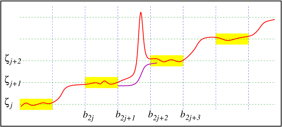
Figure 4. Glueing $Q_{*}$ with $Q_{*}^{\zeta_{j+1},\zeta_{j+2}}$.

We argue by contradiction and we suppose that

(10.4) $$\zeta\not\in\{\zeta_{j+1},\zeta_{j+2}\}.$$

Thanks to (10.2), we can exploit Lemma 6.3 and find clean points for $Q_{*}^{\zeta_{j+1},\zeta_{j+2}}$, namely

$$y_{*,1}\in(b_{2j+1}-C\rho^{-\frac{4s}{2s-1}}\,|\log\rho|,\;b_{2j+1}-1)$$

and $$y_{*,2}\in(b_{2j+2}+1,\;b_{2j+2}+C\rho^{-\frac{4s}{2s-1}}\,|\log\rho|)$$

such that

$$\sup_{x\in\left[y_{*,1}-\frac{|\log\rho|}{2},\;y_{*,1}+\frac{|\log\rho|}{2}\right]}|Q_{*}^{\zeta_{j+1},\zeta_{j+2}}(x)-\zeta_{j+1}|\leqslant\rho$$

and $$\sup_{x\in\left[y_{*,2}-\frac{|\log\rho|}{2},\;y_{*,2}+\frac{|\log\rho|}{2}\right]}|Q_{*}^{\zeta_{j+1},\zeta_{j+2}}(x)-\zeta_{j+2}|\leqslant\rho.$$

Similarly, we find clean points for $Q_{*}$, say

$$z_{*,1}\in(b_{2j},\;b_{2j}+C\rho^{-\frac{4s}{2s-1}}\,|\log\rho|)$$

and $$z_{*,2}\in(b_{2j+3}-C\rho^{-\frac{4s}{2s-1}}\,|\log\rho|,\;b_{2j+3})$$

with

$$\sup_{x\in\left[z_{*,1}-\frac{|\log\rho|}{2},\;z_{*,1}+\frac{|\log\rho|}{2}\right]}|Q_{*}(x)-\zeta_{j+1}|\leqslant\rho$$

and $$\sup_{x\in\left[z_{*,2}-\frac{|\log\rho|}{2},\;z_{*,2}+\frac{|\log\rho|}{2}\right]}|Q_{*}(x)-\zeta_{j+2}|\leqslant\rho.$$

Then we define

$$Q^{\sharp}(x):=\left\{\begin{matrix}\zeta_{j+1}&{\mbox{ if }}x<z_{*,1}-1,\\ Q_{*}(z_{*,1})\,(x-z_{*,1}+1)+\zeta_{j+1}\,(z_{*,1}-x)&{\mbox{ if }}x\in[z_{*,1}-1,z_{*,1}],\\ Q_{*}(x)&{\mbox{ if }}x\in(z_{*,1},z_{*,2}),\\ Q_{*}(z_{*,2})\,(z_{*,2}+1-x)+\zeta_{j+2}\,(x-z_{*,2})&{\mbox{ if }}x\in[z_{*,2},z_{*,2}+1],\\ \zeta_{j+2}&{\mbox{ if }}x>z_{*,2}+1.\end{matrix}\right.$$

Thus, recalling the notation in Remark 7.4 and formula (7.21),

(10.5) $$E(Q^{\sharp})\leqslant E_{(z_{*,1},z_{*,2})}(Q_{*})+\diamondsuit.$$

On the other hand, by construction $x_{*}\in(z_{*,1},z_{*,2})$, therefore

(10.6) $$Q^{\sharp}(x_{*})=Q_{*}(x_{*})\in\overline{B_{\rho}(\zeta)}.$$

Notice also that $Q^{\sharp}\in\Gamma(\zeta_{j+1},\zeta_{j+2},b_{2j+1},b_{2j+2})$. Hence, we use (10.4) and (10.6) in combination with Lemma 9.2, to find that

$$I(Q^{\sharp})\geqslant I(Q_{*}^{\zeta_{j+1},\zeta_{j+2}})+c,$$

for some $c>0$. This and (10.5) give that

(10.7) $$\begin{split}c\;&\leqslant I(Q^{\sharp})-I(Q_{*}^{\zeta_{j+1},\zeta_{j+2}})\\ &\leqslant E_{(z_{*,1},z_{*,2})}(Q_{*})-E(Q_{*}^{\zeta_{j+1},\zeta_{j+2}})+\int_{z_{*,1}}^{z_{*,2}}a(x)\,W(Q_{*}(x))\,dx-\int_{\mathbb{R}}a(x)\,W(Q_{*}^{\zeta_{j+1},\zeta_{j+2}}(x))\,dx+\diamondsuit\\ &\leqslant E_{(z_{*,1},z_{*,2})}(Q_{*})-E_{(z_{*,1},z_{*,2})}(Q_{*}^{\zeta_{j+1},\zeta_{j+2}})+\int_{z_{*,1}}^{z_{*,2}}a(x)\,\big{[}W(Q_{*}(x))-W(Q_{*}^{\zeta_{j+1},\zeta_{j+2}}(x))\big{]}\,dx+\diamondsuit.\end{split}$$

Now we define

$$\tilde{Q}(x):=\left\{\begin{matrix}Q_{*}(x)&{\mbox{ if }}x<z_{*,1},\\ Q_{*}(z_{*,1})\,(z_{*,1}+1-x)+\zeta_{j+1}\,(x-z_{*,1})&{\mbox{ if }}x\in[z_{*,1},z_{*,1}+1],\\ \zeta_{j+1}&{\mbox{ if }}x\in(z_{*,1}+1,\;y_{*,1}-1),\\ Q_{*}^{\zeta_{j+1},\zeta_{j+2}}(y_{*,1})\,(x-y_{*,1}+1)+\zeta_{j+1}\,(y_{*,1}-x)&{\mbox{ if }}x\in[y_{*,1}-1,y_{*,1}],\\ Q_{*}^{\zeta_{j+1},\zeta_{j+2}}(x)&{\mbox{ if }}x\in(y_{*,1},y_{*,2}),\\ Q_{*}^{\zeta_{j+1},\zeta_{j+2}}(y_{*,2})\,(y_{*,2}+1-x)+\zeta_{j+2}\,(x-y_{*,2})&{\mbox{ if }}x\in[y_{*,2},\;y_{*,2}+1],\\ \zeta_{j+2}&{\mbox{if }}x\in(y_{*,2}+1,\;z_{*,2}-1),\\ Q_{*}(z_{*,2})\,(x-z_{*,2}+1)+\zeta_{j+2}\,(z_{*,2}-x)&{\mbox{if }}x\in[z_{*,2}-1,\;z_{*,2}],\\ Q_{*}(x)&{\mbox{ if }}x>z_{*,2}.\end{matrix}\right.$$

Accordingly, exploiting (7.21),

$$E(\tilde{Q})\leqslant E_{(-\infty,z_{*,1})}(Q_{*})+E_{(y_{*,1},y_{*,2})}(Q_{*}^{\zeta_{j+1},\zeta_{j+2}})+E_{(z_{*,2},+\infty)}(Q_{*})+\diamondsuit.$$

Then, since $(y_{*,1},y_{*,2})\subseteq(z_{*,1},z_{*,2})$,

(10.8) $$E(\tilde{Q})\leqslant E_{(-\infty,z_{*,1})}(Q_{*})+E_{(z_{*,1},z_{*,2})}(Q_{*}^{\zeta_{j+1},\zeta_{j+2}})+E_{(z_{*,2},+\infty)}(Q_{*})+\diamondsuit.$$

Also, $\tilde{Q}\in\Gamma(\vec{\zeta},\vec{b})$, hence the minimality of $Q_{*}$ gives that

(10.9) $$I(Q_{*})\leqslant I(\tilde{Q}).$$

Furthermore

$$\int_{z_{*,1}}^{z_{*,2}}a(x)\,W(\tilde{Q}(x))\,dx = \int_{y_{*,1}}^{y_{*,2}}a(x)\,W(Q_{*}^{\zeta_{j+1},\zeta_{j+2}}(x))\,dx+\diamondsuit$$

$$\leqslant \int_{z_{*,1}}^{z_{*,2}}a(x)\,W(Q_{*}^{\zeta_{j+1},\zeta_{j+2}}(x))\,dx+\diamondsuit.$$

This, (10.8) and (10.9) imply that

$$0 \leqslant I(\tilde{Q})-I(Q_{*})$$

$$\leqslant E_{(-\infty,z_{*,1})}(Q_{*})+E_{(z_{*,1},z_{*,2})}(Q_{*}^{\zeta_{j+1},\zeta_{j+2}})+E_{(z_{*,2},+\infty)}(Q_{*})-E(Q_{*})$$

$$\qquad+\int_{z_{*,1}}^{z_{*,2}}a(x)\,\big{[}W(\tilde{Q}(x))-W(Q_{*}(x))\big{]}\,dx+\diamondsuit$$

$$\leqslant E_{(z_{*,1},z_{*,2})}(Q_{*}^{\zeta_{j+1},\zeta_{j+2}})-E_{(z_{*,1},z_{*,2})}(Q_{*})+\int_{z_{*,1}}^{z_{*,2}}a(x)\,\big{[}W(Q_{*}^{\zeta_{j+1},\zeta_{j+2}}(x))-W(Q_{*}(x))\big{]}\,dx+\diamondsuit.$$

Comparing this with (10.7), we obtain that $c\leqslant\diamondsuit$, which is a contradiction when we make $\diamondsuit$ as small as we wish (recall the notation in Remark 7.4). ∎

Now we can construct the desired multibump trajectories:

Theorem 10.3.

Let $s_{0}\in\left(\frac{1}{2},1\right)$ and $s\in[s_{0},1)$. Assume that (1.10) holds.

There exist $\varepsilon_{*}>0$ and $b_{2N-2}>b_{2N-3}>\dots>b_{2}>b_{1}\in\mathbb{R}$, possibly depending on $n$ and the structural constants of the kernel and the potential, such that if $\varepsilon\in(0,\varepsilon_{*}]$, the following statement holds.

Let $\zeta_{1}\in\mathbb{Z}^{n}$. Let $\zeta_{2}\in{\mathcal{A}}(\zeta_{1})$, $\dots$, $\zeta_{N}\in{\mathcal{A}}(\zeta_{N-1})$.

Then $Q_{*}^{\zeta_{1},\dots,\zeta_{N}}$ is a solution of (1.6).

Remark 10.4.

When $N=2$, Theorem 10.3 reduces to Theorem 9.4.

Proof of Theorem 10.3.

In view of Lemma 7.3, we need to show that the trajectory does not hit the constraints. We argue by contradiction. The idea of the proof is that: first, by Lemma 6.3, we find an integer point close to the trajectory in a clean interval; then, by Proposition 10.1, we localize the integer with respect to the two integers leading to the excursion of the orbit; this distinguishes two cases, in one case we use Proposition 8.1 to “clean” the orbit to the left (or to the right), in the other case we will be able to translate a piece of the orbit and make the energy decrease using (1.10), thus obtaining a contradiction.

The details of the argument are the following. We use the short notation $Q_{*}:=Q_{*}^{\zeta_{1},\dots,\zeta_{N}}$. By (7.3) and Lemma 7.2, we know that $I(Q_{*})$ is bounded by some $C_{*}>0$ (independently on the choice of $b_{1},\dots,b_{2N-2}$). Thus, we fix $\rho\in(0,r)$, to be taken sufficiently small, and we set

$$L:=\frac{\pi}{12\varepsilon}.$$

We suppose that $\varepsilon$ is small enough, such that

(10.10) $$L\geqslant\frac{C_{*}\,|\log\rho|}{\rho^{\frac{4s}{2s-1}}},$$

for a suitably large constant $C_{*}$, and we set $b_{1}:=L$ and then recursively

(10.11) $$\begin{split}&b_{2j}:=b_{2j-1}+22L\\ {\mbox{and }}\quad&b_{2j+1}:=b_{2j}+50L.\end{split}$$

We suppose, by contradiction, that there exists $p_{*}$ such that one of the following cases holds true:

(10.12) $$p_{*}\in(-\infty,b_{1}]{\mbox{ and }}Q_{*}(p_{*})\in\partial B_{r}(\zeta_{1}),$$

(10.13) $$p_{*}\in[b_{2j},b_{2j+1}]{\mbox{ for some\leavevmode\nobreak\ $j\in\{1,\dots,N-2\}$, and }}Q_{*}(p_{*})\in\partial B_{r}(\zeta_{j+1}),$$

(10.14) $$p_{*}\in[b_{2N-2},+\infty){\mbox{ and }}Q_{*}(p_{*})\in\partial B_{r}(\zeta_{N}).$$

We deal with the cases in (10.12) and (10.13), since the case in (10.14) is similar to the one in (10.12).

So, let us first suppose that (10.12) holds. In this case, we observe that $b_{2}-b_{1}=22L$ and so we can use Lemma 6.3 (recall (10.10) and Remark 6.4) to find an integer point $\zeta$ and some clean point $x_{*}\in(b_{1}+L,b_{1}+2L)$ for $Q_{*}(\cdot-L)$ such that

(10.15) $$\sup_{x\in\left[x_{*}-\frac{|\log\rho|}{2},\;x_{*}+\frac{|\log\rho|}{2}\right]}|Q_{*}(x-L)-\zeta|\leqslant\rho.$$

By Proposition 10.1, we know that either $\zeta=\zeta_{1}$, or $\zeta=\zeta_{2}$. But indeed $\zeta\neq\zeta_{1}$, otherwise, by (7.7) and Proposition 8.1, we would have that $|Q_{*}(x)-\zeta_{1}|\leqslant r/2$ for any $x\leqslant x_{*}$, in contradiction with the assumption taken in (10.12).

Consequently, we have that

(10.16) $$\zeta=\zeta_{2}.$$

We also remark that, by Lemma 6.3, there exists a clean point $y_{*}\in[b_{2}+1,b_{2}+1+L]$ for $Q_{*}$ such that

(10.17) $$\sup_{x\in\left[y_{*}-\frac{|\log\rho|}{2},\;y_{*}+\frac{|\log\rho|}{2}\right]}|Q_{*}(x)-\zeta_{2}|\leqslant\rho.$$

Then, we define

$$\tilde{Q}(x):=\left\{\begin{matrix}Q_{*}(x-L)&{\mbox{ if }}x\leqslant x_{*},\\ Q_{*}(x_{*}-L)\,(x_{*}+1-x)+\zeta_{2}\,(x-x_{*})&{\mbox{ if }}x\in(x_{*},\;x_{*}+1),\\ \zeta_{2}&{\mbox{ if }}x\in[x_{*}+1,\;y_{*}-1],\\ \zeta_{2}\,(y_{*}-x)+Q_{*}(y_{*})\,(x-y_{*}+1)&{\mbox{ if }}x\in[y_{*}-1,\;y_{*}],\\ Q_{*}(x)&{\mbox{ if }}x>y_{*}.\end{matrix}\right.$$

We point out that

(10.18) $$\tilde{Q}\in\Gamma(\vec{\zeta},\vec{b}).$$

Indeed, if $x\leqslant b_{1}$ then $x\leqslant x_{*}$, and also $x-L\leqslant b_{1}$, hence $\tilde{Q}(x)=Q_{*}(x-L)\in\overline{B_{r}(\zeta_{1})}$. In addition, if $x\geqslant b_{2}$, we have that $x\geqslant 23L\geqslant x_{*}+1$, and so $\tilde{Q}(x)$ always lies in a $\rho$-neighborhood of $\zeta_{2}$, up to $x=y_{*}$, or coincides with $Q_{*}$, thus completing the proof of (10.18).

From (10.18) and the minimality of $Q_{*}$, we obtain that

(10.19) $$\begin{split}0\;&\leqslant I(\tilde{Q})-I(Q_{*})\\ &\leqslant E_{(-\infty,x_{*})}(Q_{*})+E_{(y_{*},+\infty)}(Q_{*})-E(Q_{*})\\ &\qquad+\int_{-\infty}^{x_{*}}a(x)\,W(Q_{*}(x-L))\,dx-\int_{-\infty}^{y_{*}}a(x)\,W(Q_{*}(x))\,dx+\diamondsuit\\ &\leqslant\int_{-\infty}^{x_{*}-L}\big{[}a(x+L)-a(x)\big{]}\,W(Q_{*}(x))\,dx+\diamondsuit,\end{split}$$

where we used the notation in Remark 7.4 and (7.21) (we stress that (10.15), (10.16) and (10.17) give that the contributions coming from the linear interpolations are negligible).

Now we use Lemma 6.3 to find a clean point $z_{*}\in[b_{1}-L,b_{1}]$ for $Q_{*}$ and so, by (7.7) and (8.2),

$$\overline{a}\,\int_{-\infty}^{b_{1}-L}W(Q_{*}(x))\,dx\leqslant\diamondsuit.$$

We insert this into (10.19) and we conclude that

$$0\leqslant\int_{b_{1}-L}^{x_{*}-L}\big{[}a(x+L)-a(x)\big{]}\,W(Q_{*}(x))\,dx+\diamondsuit.$$

Accordingly, recalling (9.8),

(10.20) $$0\leqslant-\gamma\int_{b_{1}-L}^{x_{*}-L}W(Q_{*}(x))\,dx+\diamondsuit,$$

for some $\gamma>0$. Now, $Q_{*}(b_{1}-L)$ lies close to $\zeta_{1}$, while $Q_{*}(x_{*}-L)$ lies close to $\zeta_{2}$ (due to (10.15)): hence, by continuity and (1.7), we have that $W(Q_{*}(x))$ picks up a non-negligible contribution in a subinterval of $[b_{1}-L,x_{*}-L]$, namely

$$\int_{b_{1}-L}^{x_{*}-L}W(Q_{*}(x))\,dx\geqslant c,$$

for some $c>0$. This and (10.20) imply that $0\leqslant-c\gamma+\diamondsuit$, which is a contradiction when we make $\diamondsuit$ as small as we wish. This completes the proof of Theorem 10.3 in case (10.12).

Now we assume that (10.13) holds true. Then, by Lemma 6.3 (recall (10.10) and Remark 6.4), we know that there exist clean points $y_{*,-}\in\left[b_{2j}+\frac{L}{4},\;b_{2j}+\frac{L}{2}\right]$ and $y_{*,+}\in\left[b_{2j+1}-\frac{L}{2},b_{2j+1}-\frac{L}{4}\right]$ for $Q_{*}$, such that $|Q_{*}(y_{*,\pm})-\zeta_{j+1}|\leqslant C\rho$, with $C>0$.

Hence, by (8.3),

$$\sup_{x\in[y_{*,-},y_{*,+}]}|Q_{*}(x)-\zeta_{j+1}|\leqslant\frac{r}{2}.$$

This and (10.13) imply that $p_{*}\in[b_{2j},y_{*,-}]\cup[y_{*,+},b_{2j+1}]$.

So, we assume that

(10.21) $$p_{*}\in[b_{2j},y_{*,-}],$$

the other case being similar. We use again Lemma 6.3 to find an integer point $\zeta$ and some clean point $x_{*}\in\left[b_{2j}-\frac{L}{2},b_{2j}-\frac{L}{4}\right]$ for $Q_{*}$, such that

(10.22) $$|Q_{*}(x_{*})-\zeta|\leqslant C\rho,$$

with $C>0$. By Proposition 10.1, we know that either $\zeta=\zeta_{j}$, or $\zeta=\zeta_{j+1}$.

But it cannot be that $\zeta=\zeta_{j+1}$, otherwise, by (8.3), we would have that

$$|Q_{*}(p_{*})-\zeta_{j+1}|\leqslant\sup_{x\in[b_{2j},b_{2j+1}-L]}|Q_{*}(x)-\zeta_{j+1}|\leqslant\sup_{x\in[x_{*},y_{*,+}]}|Q_{*}(x)-\zeta_{j+1}|\leqslant\frac{r}{2},$$

in contradiction with (10.13).

Hence, we have that

(10.23) $$\zeta=\zeta_{j}.$$

Now we use again Lemma 6.3 to find a clean point $z_{*}\in\left[b_{2j-1}-\frac{L}{2},\;b_{2j-1}-\frac{L}{4}\right]$ for $Q_{*}$, such that

$$|Q_{*}(z_{*})-\zeta_{j}|\leqslant C\rho,$$

with $C>0$. We refer to Figure 5 for a sketch of the situation discussed here (of course, the picture is far from being realistic, since the horizontal scales involved are much larger than the ones depicted).

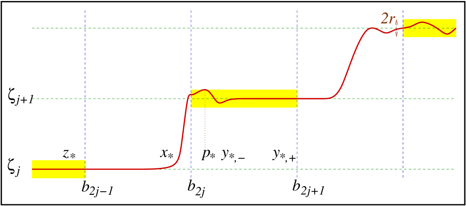
Figure 5. The points $z_{*}$, $x_{*}$, $p_{*}$, $y_{*,-}$ and $y_{*,+}$.

In this context, we can define the following two competitors: we let $Q_{1}(x)$ be

$$\left\{\begin{matrix}Q_{*}(x)&{\mbox{ if }}x\leqslant z_{*},\\ Q_{*}(z_{*})\,(z_{*}+1-x)+\zeta_{j}\,(x-z_{*})&{\mbox{ if }}x\in(z_{*},\;z_{*}+1),\\ \zeta_{j}&{\mbox{ if }}x\in[z_{*}+1,\;x_{*}-1],\\ \zeta_{j}\,(x_{*}-x)+Q_{*}(x_{*})\,(x-x_{*}+1)&{\mbox{ if }}x\in(x_{*}-1,\;x_{*}),\\ Q_{*}(x)&{\mbox{ if }}x\in[x_{*},\;y_{*,-}],\\ Q_{*}(y_{*,-})\,(y_{*,-}+1-x)+\zeta_{j+1}\,(x-y_{*,-})&{\mbox{ if }}x\in(y_{*,-},\;y_{*,-}+1),\\ \zeta_{j+1}&{\mbox{ if }}x\in[y_{*,-}+1,\;y_{*,+}-1],\\ Q_{*}(y_{*,+})\,(x-y_{*,+}+1)+\zeta_{j+1}\,(y_{*,+}-x)&{\mbox{ if }}x\in(y_{*,+}-1,\;y_{*,+}),\\ Q_{*}(x)&{\mbox{ if }}x\geqslant y_{*,+},\end{matrix}\right.$$

and $Q_{2}(x)$ be

$$\left\{\begin{matrix}Q_{1}(x)&{\mbox{ if }}x\leqslant x_{*}-1-L,\\ Q_{1}(x_{*}-1-L)\,(x_{*}-L-x)+Q_{1}(x_{*})\,(x-x_{*}+1+L)&{\mbox{ if }}x\in(x_{*}-1-L,\;x_{*}-L),\\ Q_{1}(x+L)&{\mbox{ if }}x\in[x_{*}-L,\;y_{*,-}],\\ Q_{1}(y_{*,-}+L)\,(y_{*,-}+1-x)+Q_{1}(y_{*,-}+1)\,(x-y_{*,-})&{\mbox{ if }}x\in(y_{*,-},\;y_{*,-}+1),\\ Q_{1}(x)&{\mbox{ if }}x\geqslant y_{*,-}+1.\end{matrix}\right.$$

We observe that

(10.24) $$I(Q_{1})-I(Q_{*})\leqslant\diamondsuit,$$

thanks to (7.21). Also, by inspection, one sees that $Q_{1}$, $Q_{2}\in\Gamma(\vec{\zeta},\vec{b})$. As a consequence, comparing the energy of the minimizer $Q_{*}$ with the one of the competitor $Q_{2}$ and using (10.24),

(10.25) $$\begin{split}0\;&\leqslant I(Q_{2})-I(Q_{*})\\ &=I(Q_{2})-I(Q_{1})+I(Q_{1})-I(Q_{*})\\ &\leqslant I(Q_{2})-I(Q_{1})+\diamondsuit\\ &\leqslant E_{(-\infty,x_{*}-1-L)}(Q_{1})+E_{(x_{*}-L,y_{*,-})}(Q_{1})+E_{(y_{*,-}+1,+\infty)}(Q_{1})-E(Q_{1})\\ &\qquad+\int_{x_{*}-L}^{y_{*,-}}a(x)\,W(Q_{1}(x+L))\,dx-\int_{x_{*}-1}^{y_{*,-}+1}a(x)\,W(Q_{1}(x))\,dx+\diamondsuit\\ &\leqslant\int_{x_{*}}^{y_{*,-}+L}a(x-L)\,W(Q_{1}(x))\,dx-\int_{x_{*}-1-L}^{y_{*,-}+1}a(x)\,W(Q_{1}(x))\,dx+\diamondsuit.\end{split}$$

Now we notice that if $x\in[y_{*,-}+1,\;y_{*,-}+L]\subseteq[y_{*,-}+1,\;y_{*,+}-1]$ we have that $Q_{1}(x)=\zeta_{j+1}$ and so $W(Q_{1}(x))=0$. Using this information into (10.25), we obtain that

(10.26) $$\begin{split}0\;&\leqslant\int_{x_{*}}^{y_{*,-}+1}a(x-L)\,W(Q_{1}(x))\,dx-\int_{x_{*}-1-L}^{y_{*,-}+1}a(x)\,W(Q_{1}(x))\,dx+\diamondsuit\\ &\leqslant\int_{x_{*}}^{y_{*,-}+1}\big{[}a(x-L)-a(x)\big{]}\,W(Q_{1}(x))\,dx+\diamondsuit.\end{split}$$

Now we claim that

(10.27) $$b_{2j}+L\in 24L\mathbb{N}=\frac{2\pi}{\varepsilon}\,\mathbb{N}.$$

To check this, we recall (10.11) and we perform an inductive argument. Indeed, we have that $b_{2}+L=23L+L=24L$, which checks (10.27) when $j=1$. Suppose now that (10.27) holds for some $j$ and we prove it for the index $j+1$. For this, we use (10.11) to write

$$b_{2j+2}+L=b_{2j+1}+L+22L=(b_{2j}+L)+50L+22L\in 24L\mathbb{N},$$

as desired.

This proves (10.27), from which we deduce that the interval $[b_{2j}-2L,\;b_{2j}+L]$ is a translation by $\frac{2\pi k_{j}}{\varepsilon}$ of $[21L,24L]$, for some $k_{j}\in\mathbb{N}$. This, the periodicity of $a$ and (9.9) give that, for any $x\in[b_{2j}-2L,\;b_{2j}+L]$,

(10.28) $$a(x-L)-a(x)\leqslant-\gamma,$$

for some $\gamma>0$. Now, since $[x_{*},\;y_{*,-}+1]\subseteq[b_{2j}-2L,\;b_{2j}+L]$, we have that (10.28) holds for any $x\in[x_{*},\;y_{*,-}+1]$.

Consequently, by (10.26),

(10.29) $$0\leqslant-\gamma\int_{x_{*}}^{y_{*,-}+1}W(Q_{1}(x))\,dx+\diamondsuit.$$

Since $Q_{1}(x_{*})=Q_{*}(x_{*})$, which is close to $\zeta_{j}$, by (10.22) and (10.23), and $Q_{1}(y_{*,-}+1)=\zeta_{j+1}$, it follows that the potential picks up some quantities when going from $x_{*}$ to $y_{*,-}+1$, hence (10.29) gives that $0\leqslant-c\gamma+\diamondsuit$, for some $c>0$.

This is a contradiction when we take $\diamondsuit$ appropriately small, hence we have completed the proof of Theorem 10.3.∎

Now, we obtain Theorem 1.1 from Theorem 10.3.

Appendix A Proof of Lemma 3.1

We follow the proof given in Section 8 of [DNPV12], by keeping explicit track of the constants involved.

Given $x_{0}\in J$ and $\rho>0$, we define $J_{x_{0},\rho}:=(x_{0}-\rho,x_{0}+\rho)\cap J$,

$$Q_{x_{0},\rho}:=\frac{1}{|J_{x_{0},\rho}|}\int_{J_{x_{0},\rho}}Q(y)\,dy$$

and

(A.1) $$[Q]_{s}:=\left(\sup_{{x_{0}\in J}\atop{\rho>0}}\rho^{-2s}\int_{J_{x_{0},\rho}}|Q(x)-Q_{x_{0},\rho}|^{2}\,dx\right)^{\frac{1}{2}}.$$

First of all, for any $\xi\in\mathbb{R}^{n}$ and any $\rho>0$,

(A.2) $$|\xi-Q_{x_{0},\rho}|^{2}=\frac{1}{|J_{x_{0},\rho}|^{2}}\left|\int_{J_{x_{0},\rho}}\big{[}\xi-Q(y)\big{]}\,dy\right|^{2}\leqslant\frac{1}{|J_{x_{0},\rho}|}\int_{J_{x_{0},\rho}}\big{|}\xi-Q(y)\big{|}^{2}\,dy.$$

Also, we observe that, for any $\rho\in(0,1]$,

(A.3) $$|J_{x_{0},\rho}|\in[\rho,\,2\rho].$$

Now, we claim that for any $\overline{R}\in(0,1]$ and $\underline{R}\in(0,\overline{R})$,

(A.4) $$|Q_{x_{0},\overline{R}}-Q_{x_{0},\underline{R}}|\leqslant\left(\frac{2}{\log 2\,\cdot\,\left(s-\frac{1}{2}\right)}+\sqrt{2}\right)\,[Q]_{s}\,\overline{R}^{s-\frac{1}{2}}.$$

For this, we fix $\rho_{2}>\rho_{1}>0$, with $\rho_{2}\leqslant 1$, we use (A.2) with $\xi:=Q_{x_{0},\rho_{2}}$ and $\rho:=\rho_{1}$, then we recall (A.3), and so we obtain that

(A.5) $$\begin{split}&|Q_{x_{0},\rho_{2}}-Q_{x_{0},\rho_{1}}|^{2}\leqslant\frac{1}{|J_{x_{0},\rho_{1}}|}\int_{J_{x_{0},\rho_{1}}}\big{|}Q_{x_{0},\rho_{2}}-Q(y)\big{|}^{2}\,dy\\ &\qquad\leqslant\frac{1}{\rho_{1}}\int_{J_{x_{0},\rho_{2}}}\big{|}Q_{x_{0},\rho_{2}}-Q(y)\big{|}^{2}\,dy\leqslant\frac{\rho_{2}^{2s}}{\rho_{1}}\,[Q]_{s}^{2}.\end{split}$$

Now we fix $k\in\mathbb{N}$, $k\geqslant 1$, such that

(A.6) $$\frac{1}{2^{k}}\leqslant\overline{R}^{-1}\cdot\underline{R}\leqslant\frac{1}{2^{k-1}}$$

and we define $R_{i}:=\overline{R}/2^{i}$, for any $i\in\{0,\dots,k\}$. Notice that

$$R_{k}\leqslant\underline{R}\leqslant 2R_{k},$$

due to (A.6). Then, we can use (A.5) with $\rho_{2}:=\underline{R}$ and $\rho_{1}:=R_{k}$ and find that

(A.7) $$|Q_{x_{0},\underline{R}}-Q_{x_{0},R_{k}}|\leqslant\frac{\underline{R}^{s}}{R_{k}^{\frac{1}{2}}}\,[Q]_{s}\leqslant\sqrt{2}\,\underline{R}^{s-\frac{1}{2}}\,[Q]_{s}.$$

Now we use (A.5) with $\rho_{2}:=R_{i}$ and $\rho_{1}:=R_{i+1}$ and we add up. In this way, we conclude that

(A.8) $$\begin{split}|Q_{x_{0},R_{0}}-Q_{x_{0},R_{k}}|\;&\leqslant\sum_{i=0}^{k-1}|Q_{x_{0},R_{i}}-Q_{x_{0},R_{i+1}}|\leqslant[Q]_{s}\,\sum_{i=0}^{k-1}\frac{R_{i}^{s}}{R_{i+1}^{\frac{1}{2}}}\leqslant\sqrt{2}\,\overline{R}^{s-\frac{1}{2}}\,[Q]_{s}\,\sum_{i=0}^{+\infty}\frac{1}{2^{\left(s-\frac{1}{2}\right)i}}\\ &\qquad=\sqrt{2}\,\overline{R}^{s-\frac{1}{2}}\,[Q]_{s}\,\frac{2^{s-\frac{1}{2}}}{2^{s-\frac{1}{2}}-1}\leqslant\frac{2\,\overline{R}^{s-\frac{1}{2}}\,[Q]_{s}}{\log 2\,\cdot\,\left(s-\frac{1}{2}\right)}.\end{split}$$

Hence (A.7) and (A.8) give that

$$|Q_{x_{0},R_{0}}-Q_{x_{0},\underline{R}}|\leqslant\frac{2\,\overline{R}^{s-\frac{1}{2}}\,[Q]_{s}}{\log 2\,\cdot\,\left(s-\frac{1}{2}\right)}+\sqrt{2}\,\underline{R}^{s-\frac{1}{2}}\,[Q]_{s}\leqslant\left(\frac{2}{\log 2\,\cdot\,\left(s-\frac{1}{2}\right)}+\sqrt{2}\right)\,[Q]_{s}\,\overline{R}^{s-\frac{1}{2}}.$$

Noticing now that $R_{0}=\overline{R}$, we obtain (A.4), as desired.

Now we use (A.2) with $\xi:=Q(x)$ and we integrate over $x\in J_{x_{0},\rho}$, to find that

(A.9) $$\int_{J_{x_{0},\rho}}|Q(x)-Q_{x_{0},\rho}|^{2}\,dx\leqslant\frac{1}{|J_{x_{0},\rho}|}\iint_{J_{x_{0},\rho}^{2}}\big{|}Q(x)-Q(y)\big{|}^{2}\,dx\,dy\leqslant\frac{1}{\rho}\iint_{J_{x_{0},\rho}^{2}}\big{|}Q(x)-Q(y)\big{|}^{2}\,dx\,dy,$$

where the last inequality comes from (A.3). Notice now that if $x$, $y\in J_{x_{0},\rho}\subseteq(x_{0}-\rho,x_{0}+\rho)$, then $|x-y|\leqslant 2\rho$. Hence, by (A.9),

(A.10) $$\begin{split}\int_{J_{x_{0},\rho}}|Q(x)-Q_{x_{0},\rho}|^{2}\,dx\;&\leqslant 2^{1+2s}\,\rho^{2s}\,\iint_{J_{x_{0},\rho}^{2}}\frac{\big{|}Q(x)-Q(y)\big{|}^{2}}{|x-y|^{1+2s}}\,dx\,dy\\ &\leqslant 8\,\rho^{2s}\,[Q]_{H^{s}(J)}^{2}.\end{split}$$

By comparing (A.1) with (A.10) we deduce that

(A.11) $$[Q]_{s}\leqslant\sqrt{8}\,[Q]_{H^{s}(J)}.$$

From (A.4) and (A.11), we obtain that

(A.12) $$|Q_{x_{0},\overline{R}}-Q_{x_{0},\underline{R}}|\leqslant\sqrt{8}\left(\frac{2}{\log 2\,\cdot\,\left(s-\frac{1}{2}\right)}+\sqrt{2}\right)\,[Q]_{H^{s}(J)}\,\overline{R}^{s-\frac{1}{2}}.$$

Now we claim that

(A.13) $$Q J$$ is continuous in .

For this, we use (A.12) and the assumption that $s>\frac{1}{2}$, to find that the sequence of functions $G_{\rho}(x):=Q_{x,\rho}$ is Cauchy in $L^{\infty}(J)$ and so there exists a subsequence $\rho_{j}\to 0$ such that

(A.14) $$G_{\rho_{j}} G J j\to+\infty$$ converges to some  uniformly in , as .

Now we observe that

(A.15) $$G_{\rho} J$$ is continuous in ,

for any fixed $\rho\in(0,1]$. Indeed, we know that $Q\in L^{1}(J)$ (see e.g. formula (6.21) in [DNPV12]). Therefore, if $x_{k}\in J$ and $x_{k}\to x_{\infty}$ as $k\to+\infty$, we deduce from the Dominated Convergence Theorem that

$$\lim_{k\to+\infty}\frac{1}{|J_{x_{\infty},\rho}|}\int_{J_{x_{k},\rho}}Q(y)\,dy=\frac{1}{|J_{x_{\infty},\rho}|}\int_{J_{x_{\infty},\rho}}Q(y)\,dy.$$

Accordingly

$$\lim_{k\to+\infty}\big{|}G_{\rho}(x_{k})-G_{\rho}(x_{\infty})\big{|}$$

$$\leqslant \lim_{k\to+\infty}\left|\frac{1}{|J_{x_{k},\rho}|}\int_{J_{x_{k},\rho}}Q(y)\,dy-\frac{1}{|J_{x_{\infty},\rho}|}\int_{J_{x_{k},\rho}}Q(y)\,dy\right|+\frac{1}{|J_{x_{\infty},\rho}|}\left|\int_{J_{x_{k},\rho}}Q(y)\,dy-\int_{J_{x_{\infty},\rho}}Q(y)\,dy\right|$$

$$\leqslant \lim_{k\to+\infty}\left|\frac{1}{|J_{x_{k},\rho}|}-\frac{1}{|J_{x_{\infty},\rho}|}\right|\,\int_{J}Q(y)\,dy$$

$$= 0,$$

and this gives (A.15).

By (A.14) and (A.15), we obtain that

(A.16) $$G$$ is continuous.

Now, for any $x$ in the interior of the segment $J$, we have that $J_{x,\rho_{j}}=(x-\rho_{j},x+\rho_{j})$ if $j$ is large enough and so, if $x$ is also a Lebesgue point for $Q$,

$$G(x)=\lim_{\rho_{j}\to 0}G_{\rho_{j}}(x)=\lim_{\rho_{j}\to 0}Q_{x,\rho_{j}}=\lim_{\rho_{j}\to 0}\frac{1}{|J_{x,\rho_{j}}|}\int_{J_{x,\rho_{j}}}Q(y)\,dy$$

$$\qquad=\lim_{\rho_{j}\to 0}\frac{1}{2\rho_{j}}\int_{x-\rho_{j}}^{x+\rho_{j}}Q(y)\,dy=Q(x).$$

Accordingly, $Q$ and $G$ coincide in all the Lebesgue points of the interior of $J$ and thus almost everywhere in $J$. Hence, from (A.16) (and possibly redefining $Q$ in a negligible set), we conclude that (A.13) holds true.

Thanks to (A.13), we can now send $\underline{R}\to 0$ in (A.12) and obtain that

(A.17) $$|Q_{x_{0},\overline{R}}-Q(x_{0})|\leqslant\sqrt{8}\left(\frac{2}{\log 2\,\cdot\,\left(s-\frac{1}{2}\right)}+\sqrt{2}\right)\,[Q]_{H^{s}(J)}\,\overline{R}^{s-\frac{1}{2}},$$

for any $\overline{R}\in(0,1]$ and $x_{0}\in J$.

Now we fix $X$, $Y\in J$ and we take $\overline{R}:=2|X-Y|$. Then, we obtain from (A.17) (applied with $x_{0}:=X$ and with $x_{0}:=Y$) that

(A.18) $$|Q(X)-Q_{X,\overline{R}}|+|Q_{Y,\overline{R}}-Q(Y)|\leqslant 8\,\left(\frac{2}{\log 2\,\cdot\,\left(s-\frac{1}{2}\right)}+\sqrt{2}\right)\,[Q]_{H^{s}(J)}\,|X-Y|^{s-\frac{1}{2}}.$$

Now we take $P:=\frac{X+Y}{2}$ and we notice that $(P-\overline{R},P+\overline{R})$ contains the segment joining $X$ and $Y$, which lies in $J$ and has length $\overline{R}/2$, therefore

(A.19) $$|J_{P,\overline{R}}|\geqslant\frac{{\overline{R}}}{2}.$$

Now we fix $z\in J_{P,\overline{R}}$. By (A.2), used here with $x_{0}:=X$ and $\rho:=\overline{R}$ and $\xi:=Q(z)$, we see that

$$|Q(z)-Q_{X,\overline{R}}|^{2}\leqslant\frac{1}{|J_{X,\overline{R}}|}\int_{J_{X,\overline{R}}}\big{|}Q(z)-Q(y)\big{|}^{2}\,dy.$$

Now we observe that $\overline{R}\leqslant 2$ and so, by (A.3),

$$|J_{X,\overline{R}}|\geqslant|J_{X,\overline{R}/2}|\geqslant\frac{\overline{R}}{2}$$

and therefore

$$|Q(z)-Q_{X,\overline{R}}|^{2}\leqslant\frac{\;2\;}{\overline{R}}\int_{J_{X,\overline{R}}}\big{|}Q(z)-Q(y)\big{|}^{2}\,dy\leqslant\frac{\;2\;}{\overline{R}}\int_{J_{P,2\overline{R}}}\big{|}Q(z)-Q(y)\big{|}^{2}\,dy.$$

Similarly

$$|Q(z)-Q_{Y,\overline{R}}|^{2}\leqslant\frac{\;2\;}{\overline{R}}\int_{J_{P,2\overline{R}}}\big{|}Q(z)-Q(y)\big{|}^{2}\,dy.$$

Therefore

$$|Q_{X,\overline{R}}-Q_{Y,\overline{R}}|^{2} \leqslant 2\Big{(}|Q_{X,\overline{R}}-Q(z)|^{2}+|Q(z)-Q_{Y,\overline{R}}|^{2}\Big{)}$$

$$\leqslant \frac{\;8\;}{\overline{R}}\int_{J_{P,2\overline{R}}}\big{|}Q(z)-Q(y)\big{|}^{2}\,dy.$$

Thus, by integrating over $z\in J(P,\overline{R})$ and recalling (A.19),

$$\frac{\overline{R}}{\;2\;}\,|Q_{X,\overline{R}}-Q_{Y,\overline{R}}|^{2}\leqslant\frac{\;8\;}{\overline{R}}\iint_{J_{P,2\overline{R}}^{2}}\big{|}Q(z)-Q(y)\big{|}^{2}\,dz\,dy.$$

As a consequence

$$|Q_{X,\overline{R}}-Q_{Y,\overline{R}}|^{2}\leqslant\frac{\;16\;}{\overline{R}^{2}}\iint_{{J_{P,2\overline{R}}^{2}}}\big{|}Q(z)-Q(y)\big{|}^{2}\,dz\,dy$$

$$\qquad\leqslant\frac{\;16\;}{\overline{R}^{2}}\iint_{{J_{P,2\overline{R}}^{2}}}(4\overline{R})^{1+2s}\frac{\big{|}Q(z)-Q(y)\big{|}^{2}}{|z-y|^{1+2s}}\,dz\,dy\leqslant 4^{3+2s}\,\overline{R}^{2s-1}\,[Q]^{2}_{H^{s}(J)}\leqslant 4^{6}\,|X-Y|^{2s-1}\,[Q]^{2}_{H^{s}(J)}.$$

Using this and (A.18), we obtain that

$$|Q(X)-Q(Y)| \leqslant |Q(X)-Q_{X,\overline{R}}|+|Q_{X,\overline{R}}-Q_{Y,\overline{R}}|+|Q_{Y,\overline{R}}-Q(Y)|$$

$$\leqslant 8\,\left(\frac{2}{\log 2\,\cdot\,\left(s-\frac{1}{2}\right)}+4\right)\,[Q]_{H^{s}(J)}\,|X-Y|^{s-\frac{1}{2}}.$$

This proves (3.2).

Appendix B Proof of Lemma 5.1

We notice that $Q\in C^{0,s-\frac{1}{2}}([0,1))$, thanks to Lemma 3.1, hence the condition $Q(0)=0$ is attained continuously and, more precisely, for any $y\in[0,1]$,

$$|Q(y)|\leqslant S_{0}\,[Q]_{H^{s}([0,1))}\,|y|^{s-\frac{1}{2}}.$$

Accordingly, if we define

$$V(x):=\frac{1}{x}\int_{0}^{x}\big{(}Q(x)-Q(y)\big{)}\,dy=Q(x)-\frac{1}{x}\int_{0}^{x}Q(y)\,dy,$$

we have that, for any $x\in[0,1]$,

(B.1) $$|V(x)|\leqslant S_{0}\,[Q]_{H^{s}([0,1))}\,\Big{(}|x|^{s-\frac{1}{2}}+\frac{1}{x}\int_{0}^{x}|y|^{s-\frac{1}{2}}\,dy\Big{)}=C\,S_{0}\,|x|^{s-\frac{1}{2}},$$

for some $C>0$. Moreover, by Hölder inequality,

$$|V(x)|^{2}\leqslant\frac{1}{x}\int_{0}^{x}\big{|}Q(x)-Q(y)\big{|}^{2}\,dy.$$

We also notice that if $y\in[0,x]$ then $x\geqslant x-y=|x-y|$. As a consequence,

(B.2) $$\begin{split}&\int_{0}^{\beta}x^{-2s}|V(x)|^{2}\,dx\leqslant\int_{0}^{\beta}x^{-1-2s}\left[\int_{0}^{x}\big{|}Q(x)-Q(y)\big{|}^{2}\,dy\right]\,dx\\ &\qquad\leqslant\int_{0}^{\beta}\left[\int_{0}^{x}|x-y|^{-1-2s}\big{|}Q(x)-Q(y)\big{|}^{2}\,dy\right]\,dx.\end{split}$$

Furthermore,

$$\int_{\beta}^{+\infty}x^{-2s}|V(x)|^{2}\,dx\leqslant\frac{\|V\|_{L^{\infty}((0,+\infty),\mathbb{R}^{n})}}{(2s-1)\,\beta^{2s-1}}.$$

Hence, noticing that $\|V\|_{L^{\infty}((0,+\infty),\mathbb{R}^{n})}\leqslant 2\|Q\|_{L^{\infty}((0,+\infty),\mathbb{R}^{n})}$, we find that

$$\int_{\beta}^{+\infty}x^{-2s}|V(x)|^{2}\,dx\leqslant\frac{2\|Q\|_{L^{\infty}((0,+\infty),\mathbb{R}^{n})}}{(2s-1)\,\beta^{2s-1}}.$$

From this and (B.2), we obtain that

(B.3) $$\int_{0}^{+\infty}x^{-2s}|V(x)|^{2}\,dx\leqslant\iint_{(0,\beta)\times(0,x)}\frac{\big{|}Q(x)-Q(y)\big{|}^{2}}{|x-y|^{1+2s}}\,dx\,dy+\frac{2\|Q\|_{L^{\infty}((0,+\infty),\mathbb{R}^{n})}}{(2s-1)\,\beta^{2s-1}}.$$

Now we recall a classical inequality due to Hardy, namely that for any $\alpha>0$ and any measurable function $f$, we have that

(B.4) $$\int_{0}^{+\infty}x^{-1-2\alpha}\left[\int_{0}^{x}y^{-1}\,|f(y)|\,dy\right]^{2}\,dx\leqslant\alpha^{-2}\,\int_{0}^{+\infty}y^{-1-2\alpha}\,|f(y)|^{2}\,dy.$$

To prove it, we make the substitution $y=tx$ twice and we apply the Minkowski integral inequality to the function $g(x,t):=x^{-\frac{1}{2}-\alpha}t^{-1}\,|f(tx)|$. In this way, we obtain that

$$\int_{0}^{+\infty}x^{-1-2\alpha}\left[\int_{0}^{x}y^{-1}\,|f(y)|\,dy\right]^{2}\,dx=\int_{0}^{+\infty}x^{-1-2\alpha}\left[\int_{0}^{1}t^{-1}\,|f(tx)|\,dt\right]^{2}\,dx$$

$$\qquad=\int_{0}^{+\infty}\left[\int_{0}^{1}g(x,t)\,dt\right]^{2}\,dx\leqslant\left[\int_{0}^{1}\left[\int_{0}^{+\infty}|g(x,t)|^{2}\,dx\right]^{\frac{1}{2}}\,dt\right]^{2}$$

$$\qquad=\left[\int_{0}^{1}\left[\int_{0}^{+\infty}x^{-1-2\alpha}t^{-2}\,|f(tx)|^{2}\,dx\right]^{\frac{1}{2}}\,dt\right]^{2}$$

$$\qquad=\left[\int_{0}^{1}\left[\int_{0}^{+\infty}y^{-1-2\alpha}t^{2\alpha-2}\,|f(y)|^{2}\,dy\right]^{\frac{1}{2}}\,dt\right]^{2}$$

$$\qquad=\left[\int_{0}^{1}t^{\alpha-1}\left[\int_{0}^{+\infty}y^{-1-2\alpha}\,|f(y)|^{2}\,dy\right]^{\frac{1}{2}}\,dt\right]^{2}$$

$$\qquad=\frac{1}{\alpha^{2}}\int_{0}^{+\infty}y^{-1-2\alpha}\,|f(y)|^{2}\,dy.$$

This proves (B.4).

Now we use (B.4) with $f:=V$ and $\alpha:=s-\frac{1}{2}$ and we obtain that

(B.5) $$\int_{0}^{+\infty}x^{-2s}\left[\int_{0}^{x}y^{-1}\,|V(y)|\,dy\right]^{2}\,dx\leqslant\frac{4}{(2s-1)^{2}}\,\int_{0}^{+\infty}y^{-2s}\,|V(y)|^{2}\,dy.$$

Now we define

$$Z(x):=\int_{0}^{x}y^{-1}\,V(y)\,dy$$

and we deduce from (B.5) that

(B.6) $$\int_{0}^{+\infty}x^{-2s}\,|Z(x)|^{2}\,dx\leqslant\frac{4}{(2s-1)^{2}}\,\int_{0}^{+\infty}y^{-2s}\,|V(y)|^{2}\,dy.$$

Also, recalling (B.1), we have that, for any $x\in[0,1]$, $|Z(x)|$ is controlled by $|x|^{s-\frac{1}{2}}$, which gives that $Z(0)=0$. Hence, if we define

$$F(x):=V(x)+Z(x)-Q(x),$$

recalling again (B.1) we find that $F(0)=0$. Moreover,

$$F^{\prime}(x)=Q^{\prime}(x)+\frac{1}{x^{2}}\int_{0}^{x}Q(y)\,dy-\frac{Q(x)}{x}+\frac{V(x)}{x}-Q^{\prime}(x)=0.$$

As a consequence, $F$ is constantly equal to zero in $[0,+\infty)$, which says that

$$Q(x)=V(x)+Z(x),$$

for any $x\geqslant 0$. This implies that

$$|Q(x)|^{2}\leqslant\big{(}|V(x)|+|Z(x)|\big{)}^{2}\leqslant 2\big{(}|V(x)|^{2}+|Z(x)|^{2}\big{)}.$$

Therefore, by (B.6),

$$\int_{0}^{+\infty}x^{-2s}\,|Q(x)|^{2}\,dx \leqslant 2\left(\int_{0}^{+\infty}x^{-2s}\,|V(x)|^{2}\,dx+\int_{0}^{+\infty}x^{-2s}\,|Z(x)|^{2}\,dx\right)$$

$$\leqslant 2\left(1+\frac{4}{(2s-1)^{2}}\right)\,\int_{0}^{+\infty}y^{-2s}\,|V(y)|^{2}\,dy.$$

This and (B.3) imply the thesis of Lemma 5.1.

References

- [ABM99] Francesca Alessio, Maria Letizia Bertotti, and Piero Montecchiari. Multibump solutions to possibly degenerate equilibria for almost periodic Lagrangian systems. Z. Angew. Math. Phys., 50(6):860–891, 1999. CODEN AZMPA8. ISSN 0044-2275. URL http://dx.doi.org/10.1007/s000330050184.
- [BB98] Massimiliano Berti and Philippe Bolle. Variational construction of homoclinics and chaos in presence of a saddle-saddle equilibrium. Atti Accad. Naz. Lincei Cl. Sci. Fis. Mat. Natur. Rend. Lincei (9) Mat. Appl., 9(3):167–175, 1998. ISSN 1120-6330.
- [Bes95] Ugo Bessi. Global homoclinic bifurcation for damped systems. Math. Z., 218(3):387–415, 1995. CODEN MAZEAX. ISSN 0025-5874. URL http://dx.doi.org/10.1007/BF02571911.
- [BM97] Sergey Bolotin and Robert MacKay. Multibump orbits near the anti-integrable limit for Lagrangian systems. Nonlinearity, 10(5):1015–1029, 1997. CODEN NONLE5. ISSN 0951-7715. URL http://dx.doi.org/10.1088/0951-7715/10/5/001.
- [BPSV14] Begoña Barrios, Ireneo Peral, Fernando Soria, and Enrico Valdinoci. A Widder’s type theorem for the heat equation with nonlocal diffusion. Arch. Ration. Mech. Anal., 213(2):629–650, 2014. ISSN 0003-9527. URL http://dx.doi.org/10.1007/s00205-014-0733-1.
- [Cam63] S. Campanato. Proprietà di hölderianità di alcune classi di funzioni. Ann. Scuola Norm. Sup. Pisa (3), 17:175–188, 1963.
- [CP16] Matteo Cozzi and Tommaso Passalacqua. One-dimensional solutions of non-local Allen–Cahn-type equations with rough kernels. J. Differential Equations, 260(8):6638–6696, 2016. ISSN 0022-0396. URL http://dx.doi.org/10.1016/j.jde.2016.01.006.
- [CS11] Luis Caffarelli and Luis Silvestre. Regularity results for nonlocal equations by approximation. Arch. Ration. Mech. Anal., 200(1):59–88, 2011. ISSN 0003-9527. URL http://dx.doi.org/10.1007/s00205-010-0336-4.
- [CS15] Xavier Cabré and Yannick Sire. Nonlinear equations for fractional Laplacians II: Existence, uniqueness, and qualitative properties of solutions. Trans. Amer. Math. Soc., 367(2):911–941, 2015. ISSN 0002-9947. URL http://dx.doi.org/10.1090/S0002-9947-2014-05906-0.
- [CZR91] Vittorio Coti Zelati and Paul H. Rabinowitz. Homoclinic orbits for second order Hamiltonian systems possessing superquadratic potentials. J. Amer. Math. Soc., 4(4):693–727, 1991. ISSN 0894-0347. URL http://dx.doi.org/10.2307/2939286.
- [dCN06] D. del Castillo-Negrete. Fractional diffusion models of nonlocal transport. Phys. Plasmas, 13(8):082308, 16, 2006. CODEN PHPAEN. ISSN 1070-664X. URL http://dx.doi.org/10.1063/1.2336114.
- [DFV14] Serena Dipierro, Alessio Figalli, and Enrico Valdinoci. Strongly nonlocal dislocation dynamics in crystals. Comm. Partial Differential Equations, 39(12):2351–2387, 2014. ISSN 0360-5302. URL http://dx.doi.org/10.1080/03605302.2014.914536.
- [DNPV12] Eleonora Di Nezza, Giampiero Palatucci, and Enrico Valdinoci. Hitchhiker’s guide to the fractional Sobolev spaces. Bull. Sci. Math., 136(5):521–573, 2012. ISSN 0007-4497. URL http://dx.doi.org/10.1016/j.bulsci.2011.12.004.
- [DPV15] Serena Dipierro, Giampiero Palatucci, and Enrico Valdinoci. Dislocation dynamics in crystals: a macroscopic theory in a fractional Laplace setting. Comm. Math. Phys., 333(2):1061–1105, 2015. ISSN 0010-3616. URL http://dx.doi.org/10.1007/s00220-014-2118-6.
- [GM06] Adriana Garroni and Stefan Müller. A variational model for dislocations in the line tension limit. Arch. Ration. Mech. Anal., 181(3):535–578, 2006. ISSN 0003-9527. URL http://dx.doi.org/10.1007/s00205-006-0432-7.
- [GM12] María del Mar González and Regis Monneau. Slow motion of particle systems as a limit of a reaction-diffusion equation with half-Laplacian in dimension one. Discrete Contin. Dyn. Syst., 32(4):1255–1286, 2012. ISSN 1078-0947.
- [Max97] Thomas O. Maxwell. Heteroclinic chains for a reversible Hamiltonian system. Nonlinear Anal., 28(5):871–887, 1997. CODEN NOANDD. ISSN 0362-546X. URL http://dx.doi.org/10.1016/0362-546X(95)00193-Y.
- [McL00] William McLean. Strongly elliptic systems and boundary integral equations. Cambridge University Press, Cambridge, 2000. ISBN 0-521-66332-6; 0-521-66375-X. xiv+357 pp.
- [MP12] Régis Monneau and Stefania Patrizi. Homogenization of the Peierls-Nabarro model for dislocation dynamics. J. Differential Equations, 253(7):2064–2105, 2012. CODEN JDEQAK. ISSN 0022-0396. URL http://dx.doi.org/10.1016/j.jde.2012.06.019.
- [PSV13] Giampiero Palatucci, Ovidiu Savin, and Enrico Valdinoci. Local and global minimizers for a variational energy involving a fractional norm. Ann. Mat. Pura Appl. (4), 192(4):673–718, 2013. ISSN 0373-3114. URL http://dx.doi.org/10.1007/s10231-011-0243-9.
- [PV15a] Stefania Patrizi and Enrico Valdinoci. Crystal dislocations with different orientations and collisions. Arch. Ration. Mech. Anal., 217(1):231–261, 2015. ISSN 0003-9527. URL http://dx.doi.org/10.1007/s00205-014-0832-z.
- [PV15b] Stefania Patrizi and Enrico Valdinoci. Homogenization and Orowan’s law for anisotropic fractional operators of any order. Nonlinear Anal., 119:3–36, 2015. ISSN 0362-546X. URL http://dx.doi.org/10.1016/j.na.2014.07.010.
- [Rab89] Paul H. Rabinowitz. Periodic and heteroclinic orbits for a periodic Hamiltonian system. Ann. Inst. H. Poincaré Anal. Non Linéaire, 6(5):331–346, 1989. ISSN 0294-1449. URL http://www.numdam.org/item?id=AIHPC_1989__6_5_331_0.
- [Rab94] Paul H. Rabinowitz. Heteroclinics for a reversible Hamiltonian system. Ergodic Theory Dynam. Systems, 14(4):817–829, 1994. ISSN 0143-3857. URL http://dx.doi.org/10.1017/S0143385700008178.
- [Rab97] Paul H. Rabinowitz. A multibump construction in a degenerate setting. Calc. Var. Partial Differential Equations, 5(2):159–182, 1997. ISSN 0944-2669. URL http://dx.doi.org/10.1007/s005260050064.
- [Rab00] Paul H. Rabinowitz. Connecting orbits for a reversible Hamiltonian system. Ergodic Theory Dynam. Systems, 20(6):1767–1784, 2000. ISSN 0143-3857. URL http://dx.doi.org/10.1017/S0143385700000985.
- [RCZ00] Paul H. Rabinowitz and Vittorio Coti Zelati. Multichain-type solutions for Hamiltonian systems. In Proceedings of the Conference on Nonlinear Differential Equations (Coral Gables, FL, 1999), volume 5 of Electron. J. Differ. Equ. Conf., pages 223–235 (electronic). Southwest Texas State Univ., San Marcos, TX, 2000.
- [Sér92] Éric Séré. Existence of infinitely many homoclinic orbits in Hamiltonian systems. Math. Z., 209(1):27–42, 1992. CODEN MAZEAX. ISSN 0025-5874. URL http://dx.doi.org/10.1007/BF02570817.
- [SV12] Ovidiu Savin and Enrico Valdinoci. -convergence for nonlocal phase transitions. Ann. Inst. H. Poincaré Anal. Non Linéaire, 29(4):479–500, 2012. ISSN 0294-1449. URL http://dx.doi.org/10.1016/j.anihpc.2012.01.006.