Non-Markovianity through Multipartite Correlation Measures

Abstract

We provide a characterization of memory effects in non-Markovian system-bath interactions from a quantum information perspective. More specifically, we establish sufficient conditions for which generalized measures of multipartite quantum, classical, and total correlations can be used to quantify the degree of non-Markovianity of a local quantum decohering process. We illustrate our results by considering the dynamical behavior of the trace-distance correlations in multi-qubit systems under local dephasing and generalized amplitude damping.

I Introduction

The characterization of memory effects in non-Markovian evolutions is a fundamental subject in the theory of open systems Breuer:book . Indeed, the Markovian behavior is always an idealization in the description of the quantum dynamics, with non-Markovianity being non-negligible in a number of different scenarios, such as biological Ishizaki:09 ; Rebentrost:09 ; Liang:10 ; Chen:15 or condensed matter systems Wolf:08 ; Apollaro:11 ; Haikka:12 . From an applied point of view, non-Markovian dynamics may be a resource for quantum tasks through an increase in the capacities of quantum channels Bylicka:13 . Moreover, it also exhibits applications in fault-tolerant quantum computation Aharonov:06 . Rigorously, non-Markovianity can be defined through the deviation of a dynamical evolution map from a divisible completely positive trace-preserving (CPTP) map Breuer:09 . This behavior is manifested both in entanglement Rivas:10 and in other correlation sources Luo:12 ; Haikka:13 ; Fanchini:14 ; He:14 ; Dhar:15 , providing an approach that takes advantage of quantum information tools in the open-systems realm. More specifically, non-Markovianity can be interpreted in this context as a flow of information back to the system due to its interaction with the environment, which may imply non-monotonic behavior of correlations as a function of time.

Here, we propose a general framework to characterize non-Markovianity through multipartite measures of quantum, classical, and total correlations. Recently, there has been growing interest in the investigation of correlation measures from a quantum information perspective Modi ; Celeri ; Sarandy:12 . In particular, measures for quantum correlations such as those provided by discordlike quantities and their corresponding classical counterparts have been formulated, with these quantities used as resources for implementing a variety of quantum tasks (see Ref. Modi and references therein). These measures were originally introduced in an entropic scenario by Ollivier and Zurek Ollivier:01 . In a geometric context, correlations can be defined based on the relative entropy Modi:10 , Hilbert-Schmidt norm Dakic:10 ; Bellomo:12 , trace norm Paula ; Nakano:12 , and Bures norm Spehner:13 ; Bromley . All of these distinct versions of correlation measures can be described by a unified framework in terms of a generalized distance (or pseudo distance) function Modi ; Brodutch-Modi ; EPL108 . Our approach for non-Markovianity includes all these measures as particular cases and characterizes the non-Markovian behavior by taking into account the program introduced by Rivas, Huelga, and Plenio Rivas:10 , in which an ancilla is coupled to a system which interacts with an environment. Specifically, we provide a rigorous description of the hypotheses over local dynamical maps under which quantum, classical, and total correlations can be used as measures of non-Markovianity. We illustrate the results considering the dynamics of the trace-distance correlations in qubit systems under either local dephasing or generalized amplitude damping (GAD).

II Characterizing non-Markovianity

Let us suppose a quantum process governed by a time-local master equation

$$\frac{d\rho}{dt}={\cal L}_{t}\,\rho(t),$$ (1)

where the time-dependent generator ${\cal L}_{t}$ is given by

$${\cal L}_{t}\rho(t) = -i\left[H(t),\rho(t)\right]+\sum_{i}\gamma_{i}(t)\left(A_{i}(t)\rho(t)A^{\dagger}_{i}(t)\right.$$ (2)

$$\left.-\frac{1}{2}\left\{A^{\dagger}_{i}(t)A_{i}(t),\rho(t)\right\}\right),$$

with $H(t)$ denoting the effective system Hamiltonian, $A_{i}(t)$ denoting the Lindblad operators, and $\gamma_{i}(t)$ denoting the relaxation rates. By taking the relaxation rates as positive functions, i.e., $\gamma_{i}(t)\geq 0$, the generator ${\cal L}_{t}$ assumes the Lindblad form Lindblad for each fixed $t\geq 0$. The master equation describes the dynamics of the density operator through $\rho(t)=\Phi_{t,\,\tau}\rho(\tau)$, with the CPTP map $\Phi_{t,\,\tau}$ given by $\Phi_{t,\,\tau}={\cal T}\exp\left(\int_{\tau}^{t}dt^{\prime}{\cal L}_{t^{\prime}}\right)$, with ${\cal T}$ denoting the chronological time-ordering operator. The dynamical map $\Phi_{t,\,\tau}$ then satisfies the divisibility condition $\Phi_{t,\,\tau}=\Phi_{t,\,r}\Phi_{r,\,\tau}$ $(t\geq r\geq\tau\geq 0$), which characterizes the Markovianity of the quantum process. On the other hand, for $\gamma_{i}(t)<0$, the corresponding dynamical map $\Phi_{t,\,\tau}$ may not be CPTP for intermediate time intervals and the divisibility property of the overall CPTP dynamics is violated, which characterizes a non-Markovian behavior Breuer:09 ; Rivas:10 ; Dariusz:14 .

If a function $F=F(\rho)$ is monotonically nonincreasing under divisible maps acting on $\rho$, i.e., $F(\Phi_{t,\,\tau}\rho(\tau))\leq F(\rho(\tau))$ when $\Phi_{t,\,\tau}=\Phi_{t,\,r}\Phi_{r,\,\tau}$, then $F(\rho)$ is monotonically nonincreasing with increasing time, namely, $dF(t)/dt\leq 0$. However, this is not always true for a non-Markovian process, in which the divisibility of the map is violated, with $dF(t)/dt>0$ being a straightforward non-Markovianity witness Breuer:09 . Therefore, $F(\rho)$ can be employed to point out the breakdown of Markovianity and the degree of non-Markovianity can be defined by

$$N_{F}(\Phi)=\text{max}_{\rho(0)}\int_{\frac{d}{dt}F(t)>0}{\frac{d}{dt}F(t)dt},$$ (3)

with the maximization performed over all sets of possible initial states $\rho\left(0\right)$ and the integration extended over all time intervals for which $dF(\rho)/dt>0$. Numerically, we can write

$$N_{F}(\Phi)=\textrm{max}_{\rho(0)}\sum_{i}\left[\left\{F(\tau_{i+1})-F(\tau_{i})\right\}\right],$$ (4)

where $\{(\tau_{i},\tau_{i+1})\}$ represents the set of all time intervals for which $F(t+\Delta t)>F(t)$. The maximization over $\rho(0)$ is not a trivial task. Nevertheless, it is always possible to find out lower bounds to $N_{F}(\Phi)$ by optimizing over any class of initial states, which leads to a qualitative assessment of the non-Markovianity of the map $\Phi$ Dhar:15 .

III Non-Markovianity through Correlation measures

In the general approach introduced in Refs. Modi ; Brodutch-Modi ; EPL108 , discordlike measures of quantum, classical, and total correlations of an $n$-partite system in a state $\rho$ are defined by the respective expressions

$$Q(\rho) = K\left[\rho,\,M^{-}\rho\right],$$ (5)

$$C(\rho) = K\left[M^{+}\rho,\,M^{+}\pi_{\rho}\right],$$ (6)

$$T(\rho) = K\left[\rho,\,\pi_{\rho}\right],$$ (7)

where $K\left[\rho,\sigma\right]$ denotes a real and positive function that vanishes for $\rho=\sigma$, the operator $\pi_{\rho}=\textrm{tr}_{\bar{1}}\rho\otimes\text{tr}_{\bar{2}}\rho...\otimes\text{tr}_{\bar{n}}\rho$ represents the product of the local marginals of $\rho$, and $M^{-}\rho$ and $M^{+}\rho$ are classical states obtained through measurement maps $M^{-}$ and $M^{+}$ that minimize $Q$ and maximize $C$, respectively. In particular, they will be taken here as local $n$-partite maps $M^{\pm}=M^{\pm}_{1}\otimes M^{\pm}_{2}\cdots\otimes M^{\pm}_{n}$, where $M^{\pm}_{i}\neq\mathbb{I}$ or $M^{\pm}_{i}=\mathbb{I}$ depending on whether the ith partition is measured or unmeasured. Furthermore, we will define the measurements $\{M^{\pm}_{i}\neq\mathbb{I}\}$ as optimized complete sets of local orthogonal projectors. Since orthogonal projective measurements are adopted, we have $M^{\pm}_{i}M^{\pm}_{i}\rho=M^{\pm}_{i}\rho$.

The correlation measures in Eqs. (5)-(7) are expected to obey the following set of fundamental criteria Modi ; Brodutch-Modi ; EPL108 : (i) product states have no correlations, (ii) all correlations are invariant under local unitary operations, (iii) all correlations are non-negative, (iv) total correlations are nonincreasing under local quantum channels (CPTP maps), (v) classical states have no quantum correlations, and (vi) quantum correlations are nonincreasing under local quantum channels over unmeasured subsystems EPL108 . In order to satisfy the requirements above, we restrict $K$ to be positive and unitary invariant. Moreover, we also require $K$ to be contractible under CPTP maps $\Phi$ EPL108 , i.e.,

$$K[\Phi\rho,\Phi\sigma]\leq K[\rho,\sigma]\,\,\,\,\,\,(\forall\rho,\sigma).$$ (8)

In particular, a variety of such functions $K$ can be adopted as, for instance, the trace distance $K(\rho,\sigma)=\mathrm{tr}|\rho-\sigma|$.

In this work, we will consider multipartite correlated quantum systems, such as that illustrated in Fig. 1. In particular, we will consider local dynamical maps $\Phi=\Phi_{1}\otimes\Phi_{2}\cdots\otimes\Phi_{n}$. In this scenario, we can show that a non-monotonic behavior of the correlations $Q(\rho)$, $C(\rho)$, and $T(\rho)$ as a function of time may provide a direct measure of the degree of non-Markovianity $N_{F}(\Phi)$, with $F=Q,C,$ or $T$. This result is contained in Theorem 1 below.

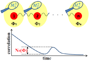
Figure 1: Illustration of the degree of non-Markovianity $N_{F}(\Phi)$ via locally measured states.

Theorem 1.

Consider a quantum evolution driven by a local dynamical map $\Phi=\bigotimes_{i=1}^{n}\Phi_{i}$. Then, assuming that $K$ is contractible under CPTP maps, it follows that (i) $N_{T}(\Phi)$ is a measure of non-Markovianity and (ii) $N_{Q}(\Phi)$ and $N_{C}(\Phi)$ are measures of non-Markovianity for local measurements $M^{\pm}=\bigotimes_{i=1}^{n}M^{\pm}_{i}$ such that $M^{\pm}_{i}=\mathbb{I}$ when $\Phi_{i}\neq\mathbb{I}\,$.

Proof.

We begin by using $\Phi=\bigotimes_{i=1}^{n}\Phi_{i}$. Then, by adopting $t\geq\tau\geq 0$, we write $\rho(t)=\Phi_{t,\tau}\rho(\tau)=\bigotimes_{i}\Phi_{i\,t,\tau\,}\rho(\tau)$. Moreover, for local CPTP maps, we have the relation $\pi_{\Phi_{t,\tau}\rho(\tau)}=\Phi_{t,\tau}\pi_{\rho(\tau)}$. (i) Thus, let us consider $N_{T}(\Phi)$. A generalized total correlation measure can be written as $T(t)=K\left[\rho(t),\,\pi_{\rho(t)}\right]=K\left[\Phi_{t,\tau}\rho(\tau),\,\Phi_{t,\tau}\pi_{\rho(\tau)}\right]$. Imposing the condition that $K$ is contractible under CPTP maps, we have $K\left[\Phi_{t,\tau}\rho(\tau),\,\Phi_{t,\tau}\pi_{\rho(\tau)}\right]\leq K\left[\rho(\tau),\,\pi_{\rho(\tau)}\right]=T(\tau)$. Hence, $T(t)\leq T(\tau)$. (ii) Let us now take $N_{Q}(\Phi)$ and $N_{C}(\Phi)$. A generalized quantum correlation measure can be written as $Q(t)=K\left[\rho(t),M_{t}^{-}\rho(t)\right]$, where we are considering $M_{t}^{-}=\bigotimes_{i}M^{-}_{i\,t}$ with $M^{-}_{i}=\mathbb{I}$ when $\Phi_{i}\neq\mathbb{I}$ (consequently, $M^{-}\Phi=\Phi M^{-}$). As $M_{\tau}^{-}$ does not necessarily minimize $Q(t)$, we can write $Q(t)\leq K\left[\rho(t),M_{\tau}^{-}\rho(t)\right]=K\left[\Phi_{t,\tau}\rho(\tau),\Phi_{t,\tau}M_{\tau}^{-}\rho(\tau)\right]$. By taking $\Phi_{i\,t,\tau}$ as a CPTP map and imposing the condition that $K$ is contractible under CPTP maps, we obtain $K\left[\Phi_{t,\tau}\rho(\tau),\Phi_{t,\tau}M_{\tau}^{-}\rho(\tau)\right]\leq K\left[\rho(\tau),M_{\tau}^{-}\rho(\tau)\right]=Q(\tau)$. Hence, $Q(t)\leq Q(\tau)$. Next, let us consider $N_{C}(\Phi)$. A generalized classical correlation measure can be written as $C(t)=K\left[M_{t}^{+}\rho(t),M_{t}^{+}\pi_{\rho(t)}\right]$, where we are considering $M_{t}^{+}=\bigotimes_{i}M^{+}_{i\,t}$ with $M^{+}_{i}=\mathbb{I}$ when $\Phi_{i}\neq\mathbb{I}$ (consequently, $M^{+}\Phi=\Phi M^{+}$). Then, imposing the condition that $K$ is contractible under CPTP maps, we can write $C(t)=K\left[\Phi_{t\,,\tau}M_{t}^{+}\rho(\tau),\Phi_{t\,,\tau}M_{t}^{+}\pi_{\rho(\tau)}\right]\leq K\left[M_{t}^{+}\rho(\tau),M_{t}^{+}\pi_{\rho(\tau)}\right]$. As $M_{t}^{+}$ does not necessarily maximize $C(\tau)$, then $K\left[M_{t}^{+}\rho(\tau),M_{t}^{+}\pi_{\rho(\tau)}\right]\leq K\left[M_{\tau}^{+}\rho(\tau),M_{\tau}^{+}\pi_{\rho(\tau)}\right]=C(\tau)$. Hence, $C(t)\leq C(\tau)$. ∎

We observe that Theorem 1 ensures $N_{Q}(\Phi)$ and $N_{C}(\Phi)$ as measures of non-Markovianity by assuming that the subsystems under decoherence are unmeasured, i.e., $M^{\pm}_{i}=\mathbb{I}$ when $\Phi_{i}\neq\mathbb{I}$. The measurements are then performed over ancillary states that are effectively free of decoherence. This requirement is unnecessary for $N_{T}(\Phi)$ since it is a measurement-independent quantifier. An effective isolation of an ancilla to probe non-Markovianity has been experimentally achieved in several scenarios (see, e.g., Refs. Xu:13 ; Bernardes:15 ). More generally, it can be approximately assumed when the relaxation times of the ancillary subsystem are much larger than those of the principal subsystem. Similarly, it also happens when the multi-local dynamical map can be written as an effective transformation where only part of the subsystems undergoes decoherence [see Eq. (12) for a bipartite example in Sec. IV B].

IV Applications

IV.1 Trace-norm correlations for two-qubit X states

Let us consider correlations based on the Schatten 1-norm (trace-norm) and projective measurements operating over one qubit within a two-qubit system, i.e., $K\left[\rho,\sigma\right]=\mathrm{tr}|\rho-\sigma|$ and $M^{\pm}=M_{1}^{\pm}\otimes\mathbb{I}$. By adopting these conditions, $Q(\rho)=\mathrm{tr}\left|\rho-M_{1}^{-}\otimes\mathbb{I}\,\rho\right|$ is then the trace-norm geometric quantum discord, as introduced in Refs. Paula ; Nakano:12 , with $C(\rho)=\mathrm{tr}\left|M_{1}^{+}\otimes\mathbb{I}\,\left(\rho-\pi_{\rho}\right)\right|$ and $T(\rho)=\mathrm{tr}\left|\rho-\pi_{\rho}\right|$ being the corresponding classical and total correlations EPL108 . The trace-norm geometric quantum and classical correlations have been experimentally discussed in Refs. Silva:13 ; PRL:13 . We will consider initial density operators restricted to the X states, i.e.,

$$\rho(0)=\frac{1}{4}\left[\mathbb{I}\otimes\mathbb{I}+\sum_{i=1}^{3}c_{i}\,\sigma_{i}\otimes\sigma_{i}+c_{4}\mathbb{I}\otimes\sigma_{3}+c_{5}\sigma_{3}\otimes\mathbb{I}\right],$$ (9)

where $\{\sigma_{i}\}$ represent the Pauli matrices and $\{c_{i}=c_{i}(0)\}$ are the initial correlation parameters. These states represent, for example, the general form of reduced density operators of arbitrary quantum spin chains with $Z_{2}$ (parity) symmetry (for a review see, e.g., Ref. Sarandy:12 ). The trace-norm correlation measures have been analytically developed for a general X state Ciccarello:14 ; Paola:15 , reading

$$Q = \sqrt{\frac{ac-bd}{a+c-b-d}},$$

$$C = \text{max}\left\{|c_{1}|,|c_{2}|,|c_{3}-c_{4}c_{5}|\right\},$$

$$T = \max\left\{C,\tfrac{1}{2}\left(|c_{1}|+|c_{2}|+|c_{3}-c_{4}c_{5}|\right)\right\},$$ (10)

where $a=\text{max}\{c_{3}^{2},d+c_{5}^{2}\}$, $b=\text{min}\{c,c_{3}^{2}\}$, $c=\text{max}\{c_{1}^{2},c_{2}^{2}\}$, and $d=\text{min}\{c_{1}^{2},c_{2}^{2}\}$.

IV.2 Two-qubit state under dephasing via a time-local master equation

Let us start by focusing on a dynamical map of the form $\Phi=\Phi_{1}\otimes\Phi_{2}$, where

$$\Phi_{j}\rho_{j}={\frac{1+f_{j}(t)}{2}}\rho_{j}\,\,+\,\,{\frac{1-f_{j}(t)}{2}}\sigma_{3}\rho_{j}\sigma_{3},$$ (11)

with $f_{j}(t)=\text{exp}\left[-2\int_{0}^{t}\gamma_{j}(\tau)d\tau\right]$. This represents a local dephasing channel acting over subsystem $j$, which can be derived from Eq. (1) by taking $H=-\left(\sigma_{z}^{1}+\sigma_{z}^{2}\right)/2$ and $A_{j}=\sigma_{z}^{j}$ ($j=1,2$). For simplicity, the time-dependent decoherence rates associated with each subsystem will be chosen to be the same, namely, $\gamma_{1}(t)=\gamma_{2}(t)$ such that $f_{1}(t)=f_{2}(t)$. The map $\Phi_{j}$ preserves the X state form of $\rho$, with $\{c_{1}(t),c_{2}(t),c_{3}(t),c_{4}(t),c_{5}(t)\}=\{c_{1}f_{k}(t),c_{2}f_{k}(t),c_{3},c_{4},c_{5}\}$. Moreover, we can write

$$\Phi=\Phi_{1}\otimes\Phi_{2}=\Phi^{eff}\otimes\mathbb{I}=\mathbb{I}\otimes\Phi^{eff},$$ (12)

where $\Phi^{eff}$ is an effective dephasing channel with $f(t)=f_{1}(t)f_{2}(t)=\text{exp}\left[-2\int_{0}^{t}\gamma(\tau)d\tau\right]$, with $\gamma(\tau)=\gamma_{1}(\tau)+\gamma_{2}(\tau)=2\gamma_{1}(t)$, such that $\{c_{1}(t),c_{2}(t),c_{3}(t),c_{4}(t),c_{5}(t)\}=\{c_{1}f(t),c_{2}f(t),c_{3},c_{4},c_{5}\}$. Therefore, $Q(t)$, $C(t)$, or $T(t)$ can be used to characterize non-Markovianity, as provided by Theorem 1. In the Markovian regime, which takes place when $\gamma(t)\geq 0$ for all $t\geq 0$, we have $df(t)/dt\leq 0$. Consequently, we have $dQ(t)/dt\leq 0$, $dC(t)/dt\leq 0$, and $dT(t)/dt\leq 0$.

In order to quantify the non-Markovianity of the dynamical map $\Phi=\Phi_{1}\otimes\Phi_{2}$, we will first consider the classical correlation. Thus, we replace $F(t)$ by $C(t)$ in Eq. (3). The condition $dC(t)/dt>0$ occurs only if $C(t)>|c_{3}(0)-c_{4}(0)c_{5}(0)|$ and $\gamma(t)<0$. Under this condition, $dC(t)/dt=-2\text{max}\{|c_{1}(0)|,|c_{2}(0)|\}\gamma(t)f(t)$ and the maximization in Eq. (3) is achieved when $c_{3}(0)-c_{4}(0)c_{5}(0)=0$ and $\text{max}\{|c_{1}(0)|,|c_{2}(0)|\}=1$. Thus, we find

$$N_{C}(\Phi)=-2\int_{\gamma(t)<0}{\gamma(t)f(t)dt}.$$ (13)

By taking $\rho(0)$ as a maximally entangled state, we obtain the same estimation of the non-Markovianity degree via total or quantum correlation. In fact, we have for the four Bell states $\left|c_{1}\right|=\left|c_{2}\right|=\left|c_{3}\right|=1$ and $c_{4}=c_{5}=0$ such that $T(t)=\max\{1,f(t)+\frac{1}{2}\}$ and $Q(t)=f(t)$. As $df(t)/dt=-2\gamma(t)f(t)$ and $f(t)>0$, we conclude that $dT(t)/dt>0$ or $dQ(t)/dt>0$ is equivalent to $\gamma(t)<0$. Under this condition, $f(t)>1$ and $dT(t)/dt=dQ(t)/dt=-2\gamma(t)f(t)$, which leads to

$$N_{T}(\Phi)=N_{Q}(\Phi)=N_{C}(\Phi).$$ (14)

The degree of non-Markovianity found here via trace-distance correlation measures is then consistent with previous results for measures of non-Markovianity Breuer:09 ; Dhar:15 ; Vacchini ; Luo:12 .

IV.3 Two-qubit state under GAD via the Lindblad rate equation

Let us now illustrate the signature of non-Markovianity for two qubits under local GAD, which will be described in the open-system framework developed in Ref. AAPRA74 based on a Lindblad rate equation. In this scenario, the density matrix in Eq.(1) is replaced by

$$\rho(t)=\sum^{R_{max}}_{R=1}\rho_{R}(t),$$ (15)

where each auxiliary (unnormalized) operator $\rho_{R}$ defines the system dynamics given that the reservoir is in the $R$-configurational bath state, with $R_{max}$ being the number of configurational states of the environment. The probability that the environment is in a given state at time $t$ reads $P_{R}(t)=\mathrm{tr}[\rho_{R}(t)]$, and the set of states $\{\rho_{R}(t)\}$ encodes both the system dynamics and the fluctuations of the environment AAPRA74 ; HPPRA75 . Then, we model the environment as being characterized by a two-dimensional configurational space ($R_{max}=2$), which only affects the decay rates of the system. Each state follows by itself a Lindblad rate equation

$$\frac{d\rho_{1}(t)}{dt} = -i[H_{1},\rho_{1}(t)]+\bar{\gamma}^{A}_{1}\mathcal{L}^{A}\rho_{1}(t)+\bar{\gamma}^{B}_{1}\mathcal{L}^{B}\rho_{1}(t)$$ (16)

$$- \phi_{21}\rho_{1}(t)+\phi_{12}\rho_{2}(t),$$

$$\frac{d\rho_{2}(t)}{dt} = -i[H_{2},\rho_{2}(t)]+\bar{\gamma}^{A}_{2}\mathcal{L}^{A}\rho_{2}(t)+\bar{\gamma}^{B}_{2}\mathcal{L}^{B}\rho_{2}(t)$$ (17)

$$- \phi_{21}\rho_{2}(t)+\phi_{12}\rho_{1}(t),$$

where the structure of the superoperator $\mathcal{L}$ for the GAD channel is given by

$$\mathcal{L}^{A,B}\rho_{R}=\left(-\frac{\sigma^{\dagger A,B}\sigma^{A,B}\,\rho_{R}}{2}-\frac{\rho_{R}\,\sigma^{\dagger A,B}\sigma^{A,B}}{2}+\sigma^{\dagger A,B}\rho_{R}\sigma^{A,B}\right).$$ (18)

The first lines of Eqs. (16) and (17) define the unitary and dissipative dynamics for the two-qubit system, given that the bath is in configurational state 1 and configurational state 2, respectively. The constants $\{\bar{\gamma}^{A}_{1,2},\bar{\gamma}^{B}_{1,2}\}$ are the natural decay rates of the system associated with each reservoir state. The positivity of the density matrix will be ensured as long as these decoherence coefficients obey $\bar{\gamma}^{A\,B}_{1,2}\geq 0$ AAPRA74 ; budini43 . On the other hand, the second line of Eqs. (16) and (17) describes transitions between the configurational states of the environment (with rates $\phi_{12}$ and $\phi_{21}$) budini43 . For simplicity, the decay rates associated with each subsystem will be chosen to be the same, namely, $\bar{\gamma}^{A}_{1}=\bar{\gamma}^{B}_{1}\equiv\bar{\gamma}_{1}$ and $\bar{\gamma}^{A}_{2}=\bar{\gamma}^{B}_{2}\equiv\bar{\gamma}_{2}$. Moreover, we define the characteristic dimensionless parameters

$$\epsilon=\frac{\bar{\gamma}_{1}}{\bar{\gamma}_{1}+\bar{\gamma}_{2}},\quad\eta=\frac{\phi_{12}}{\phi_{12}+\phi_{21}}\quad v=\frac{\phi_{12}+\phi_{21}}{\bar{\gamma}_{1}+\bar{\gamma}_{2}},$$ (19)

where $\epsilon,\eta\in[0,1]$ and $v\in[0,\infty)$. We will analyze the system in the limit of either fast or slow environmental fluctuations. The fast limit of environmental fluctuations occurs when the reservoir fluctuations are much faster than the average decay rates of the system, namely, $\{\phi_{R^{\prime}R}\}\gg\{\bar{\gamma}_{R}\}$ ($v\gg 1$), which implies that the system exhibits Markovian behavior. On the other hand, when the bath fluctuations are much slower than the average decay rate, namely, $\{\phi_{R^{\prime}R}\}\ll\{\bar{\gamma}_{R}\}$ ($v\ll 1$), the system is in the limit of slow environmental fluctuations. The signatures of non-Markovianity will be provided by the total correlation, which has the advantages of avoiding both extremization procedures and further requirements over the dynamical map. The non-Markovian behavior can then be witnessed in Fig. 2, which shows the temporal evolution of the total correlation for several values of $v$, where we have taken $\epsilon=0.92$, $\eta=0,5$, and an initial X state described by $c_{1}=0.20,c_{2}=-0.20,c_{3}=0.60,c_{4}=0.50$, and $c_{5}=0.70$.

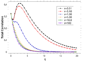
Figure 2: Total correlation as a function of $\tau=(\bar{\gamma}_{A}+\bar{\gamma}_{B})t$ for a two-qubit system under a non-Markovian GAD channel. The initial state is in the X form, with $c_{1}=0.20$, $c_{2}=-0.20$, $c_{3}=0.60$, $c_{4}=0.50$, and $c_{5}=0.70$. We have also taken $\epsilon=0.92$ and $\eta=0.5$. The non-monotonic behavior gets pronounced as we decrease $v$ from the Markovian regime ($v\gg 1$) towards the non-Markovian regime.

For the fast limit, the decay of the total correlation is a monotonically decreasing function, which corresponds to a Markovian evolution. Otherwise, when the system is subject to a non-Markovian evolution (slow limit), the total correlation shows a non-monotonic evolution, which gets more pronounced as we decrease $v$. The degree of non-Markovianity $N_{T}(v)$ can be rigorously obtained from Eq.(4) by a maximization over all initial states. On the other hand, a lower bound for $N_{T}(v)$ can be directly obtained from Fig. 2 through the height of the non-monotonic sector as a function of $v$.

IV.4 Multipartite entangled state under local dephasing

Consider an $n$-partite system initially in the Greenberger-Horne-Zeilinger (GHZ) state, i.e., a maximally entangled state of the form

$$\rho=\frac{1}{2}\left(\left|0\right\rangle^{n}\left\langle 0\right|^{n}+\left|0\right\rangle^{n}\left\langle 1\right|^{n}+\left|1\right\rangle^{n}\left\langle 0\right|^{n}+\left|1\right\rangle^{n}\left\langle 1\right|^{n}\right),$$ (20)

where $\left|k\right\rangle^{n}=\left|k\right\rangle_{1}\otimes\left|k\right\rangle_{2}\otimes\cdots\otimes\left|k\right\rangle_{n}$ $\left(k=0,\,1\right)$. By applying a dynamical map $\Phi=\Phi_{1}\otimes\Phi_{2}\otimes\cdots\otimes\Phi_{n}$ over the GHZ state and choosing $\Phi_{i}$ as a local dephasing channel as in Eq. (11), we get

$$\rho(t)=\frac{1}{2}\left(\left|0\right\rangle^{n}\left\langle 0\right|^{n}+f(t)\left|0\right\rangle^{n}\left\langle 1\right|^{n}+f(t)\left|1\right\rangle^{n}\left\langle 0\right|^{n}+\left|1\right\rangle^{n}\left\langle 1\right|^{n}\right),$$ (21)

where $f(t)=\text{exp}\left[-2\int_{0}^{t}\gamma(\tau)d\tau\right]$, with $\gamma(t)=\sum_{i=1}^{n}{\gamma_{i}(t)}$ denoting the sum of the time-dependent decoherence rates. We will consider the multipartite total correlation as the non-Markovianity quantifier and use the GHZ state to provide a lower bound for $N_{T}(\Phi)$. The product of the local marginals of $\rho(t)$ is given by $\pi_{\rho(t)}=\mathbb{I}/2^{n}$, and the eigenvalues of the operator $\rho(t)-\pi_{\rho(t)}$ are

$$\lambda_{i} = -2^{-n}\,\,\,\,\,\left(1\leq i\leq 2^{n}-2\right),$$

$$\lambda_{2^{n}-1} = \frac{1}{2}\left(1-2^{1-n}-f\right),$$

$$\lambda_{2^{n}} = \frac{1}{2}\left(1-2^{1-n}+f\right).$$ (22)

Therefore, $T(t)=\sum_{i}^{2^{n}}\left|\lambda_{i}\right|$ or $T(t)=1-2^{1-n}+\max\{1-2^{1-n},f(t)\}.$ We have $dT/dt=0$ for $f(t)\leq 1-2^{1-n}$ and $dT/dt=-2\gamma(t)f(t)$ for $f(t)>1-2^{1-n}$. Since $f(t)>0$, we conclude that $dT/dt>0$ is equivalent to the condition $\gamma(t)<0$. Moreover, $f(t)>1$ [consequently, $f(t)>1-2^{n-1}$] when $\gamma(t)<0$. Thus, we find a generalization of the result in Eq.(13):

$$N_{T}(\Phi)=\int_{\frac{d}{dt}T(t)>0}{\frac{d}{dt}T(t)dt}=-2\int_{\gamma(t)<0}{\gamma(t)f(t)dt}.$$ (23)

V Conclusion

We have introduced a unified framework based on generalized quantum, classical, and total correlation measures to characterize the non-Markovianity of local dynamical maps over multipartite quantum systems. This approach establishes sufficient conditions under which each class of correlation can be used to determine the degree of non-Markovian behavior. We illustrated our results for different master-equation methods and for different sources of decoherence. We expect applications in experimental setups for which correlations may be accessible to the observer. In addition, the vanishing of entanglement for high-temperature regimes Werlang:10 or for distant neighbors within a composite system Maziero:PLA may also motivate the use of generalized correlations as a tool to characterize non-Markovianity. Further applications include the assessment of other approaches beyond Markovianity (see, e.g., Ref. Shabani:05 ) and of additional axioms over correlation functions (see, e.g., Refs. Cianciaruso ; Hu:12 ). These topics are left for future research.

References

- (1) H.-P. Breuer and F. Petruccione, The Theory of Open Quantum Systems (Oxford University Press, New York, 2002).
- (2) A. Ishizaki and G. R. Fleming, J. Chem. Phys. 130, 234110 (2009); 130, 234111 (2009).
- (3) P. Rebentrost, R. Chakraborty, and A. Aspuru-Guzik, J. Chem. Phys. 131, 184102 (2009).
- (4) X.-T. Liang, Phys. Rev. E 82, 051918 (2010).
- (5) H.-B. Chen, N. Lambert, Y.-C. Cheng, Y.-N. Chen, and F. Nori, Sci. Rep. 5, 12753 (2015).
- (6) M. M. Wolf, J. Eisert, T. S. Cubitt, and J. I. Cirac, Phys. Rev. Lett. 101, 150402 (2008).
- (7) T. J. G. Apollaro, C. Di Franco, F. Plastina, and M. Paternostro Phys. Rev. A 83, 032103 (2011).
- (8) P. Haikka, J. Goold, S. McEndoo, F. Plastina, and S. Maniscalco, Phys. Rev. A 85, 060101(R) (2012).
- (9) B. Bylicka, D. Chruscinski, and S. Maniscalco, Sci. Rep. 4, 5720 (2014).
- (10) D. Aharonov, A. Kitaev, and J. Preskill, Phys. Rev. Lett. 96, 050504 (2006).
- (11) H.-P. Breuer, E.-M. Laine, and J. Piilo, Phys. Rev. Lett. 103, 210401 (2009).
- (12) A. Rivas, S. F. Huelga, and M. B. Plenio, Phys. Rev. Lett. 105, 050403 (2010).
- (13) S. Luo, S. Fu, and H. Song, Phys. Rev. A 86, 044101 (2012).
- (14) P. Haikka, T. H. Johnson, and S. Maniscalco, Phys. Rev. A 87, 010103(R) (2013).
- (15) F. F. Fanchini, G. Karpat, B. Çakmak, L. K. Castelano, G. H. Aguilar, O. Jiménez Farías, S. P. Walborn, P. H. Souto Ribeiro, and M. C. de Oliveira, Phys. Rev. Lett. 112, 210402 (2014).
- (16) Z. He, C. Yao, Q. Wang, and J. Zou, Phys. Rev. A 90, 042101 (2014).
- (17) H. S. Dhar, M. N. Bera, and G. Adesso, Phys. Rev. A 91, 032115 (2015).
- (18) K. Modi, A. Brodutch, H. Cable, T. Paterek, and V. Vedral, Rev. Mod. Phys. 84, 1655 (2012).
- (19) L. C. Céleri, J. Maziero, and R. M. Serra, Int. J. Quantum Inf. 9, 1837 (2011).
- (20) M. S. Sarandy, T. R. de Oliveira, and L. Amico, Int. J. Mod. Phys. B 27, 1345030 (2013).
- (21) H. Ollivier and W. H. Zurek, Phys. Rev. Lett. 88, 017901 (2001).
- (22) K. Modi, T. Paterek, W. Son, V. Vedral, and M. Williamson, Phys. Rev. Lett. 104, 080501 (2010).
- (23) B. Dakić, V. Vedral, and C. Brukner, Phys. Rev. Lett. 105, 190502 (2010).
- (24) B. Bellomo, G. L. Giorgi, F. Galve, R. Lo Franco, G. Compagno, and R. Zambrini, Phys. Rev. A 85, 032104 (2012).
- (25) F. M. Paula, T. R. de Oliveira, and M. S. Sarandy, Phys. Rev. A 87, 064101 (2013).
- (26) T. Nakano, M. Piani, and G. Adesso, Phys. Rev. A 88, 012117 (2013).
- (27) D. Spehner and M. Orszag, New J. Phys. 15, 103001 (2013).
- (28) T. R. Bromley, M. Cianciaruso, R. Lo Franco, and G. Adesso, J. Phys. A 47, 405302 (2014).
- (29) A. Brodutch and K. Modi, Quantum Inf. Comput. 12, 0721 (2012).
- (30) F. M. Paula, A. Saguia, T. R. de Oliveira, and M. S. Sarandy, Europhys. Lett. 108, 10003 (2014).
- (31) V. Gorini, A. Kossakowski, and E. C. G. Sudarshan, J. Math. Phys. (Melville, N.Y., U. S.) 17, 821 (1976).
- (32) D. Chruscinski and S. Maniscalco, Phys. Rev. Lett. 112, 120404 (2014).
- (33) J.-S. Xu, K. Sun, C.-F. Li, X.-Y. Xu, G.-C. Guo, E. Andersson, R. Lo Franco, and G. Compagno, Nature Commun. 4, 2851 (2013).
- (34) N. K. Bernardes, A. Cuevas, A. Orieux, C. H. Monken, P. Mataloni, F. Sciarrino, and M. F. Santos, Sci. Rep. 5, 17520 (2015).
- (35) I. A. Silva, D. Girolami, R. Auccaise, R. S. Sarthour, I. S. Oliveira, T. J. Bonagamba, E. R. deAzevedo, D. O. Soares-Pinto, and G. Adesso, Phys. Rev. Lett. 110, 140501 (2013).
- (36) F. M. Paula, I. A. Silva, J. D. Montealegre, A. M. Souza, E. R. deAzevedo, R. S. Sarthour, A. Saguia, I. S. Oliveira, D. O. Soares-Pinto, G. Adesso, and M. S. Sarandy, Phys.Rev. Lett. 111, 250401 (2013).
- (37) P. C. Obando, F. M. Paula, and M. S. Sarandy, Phys. Rev. A 92, 032307 (2015).
- (38) F. Ciccarello, T. Tufarelli, and V. Giovannetti, New J. Phys. 16, 013038 (2014).
- (39) B. Vacchini, A. Smirne, E.-M. Laine, J. Piilo, and H.-P. Breuer, New J. Phys. 13, 093004 (2011).
- (40) A. A. Budini, Phys. Rev. A 74, 053815 (2006).
- (41) H.-P. Breuer, Phys. Rev. A 75, 022103 (2007).
- (42) A. A. Budini, J. Phys. B 43, 115501, (2010).
- (43) T. Werlang, C. Trippe, G. A. P. Ribeiro, and G. Rigolin, Phys. Rev. Lett. 105, 095702 (2010).
- (44) J. Maziero, L. C. Céleri, R. M. Serra, and M. S. Sarandy, Phys. Lett. A 376, 1540 (2012).
- (45) A. Shabani and D. A. Lidar, Phys. Rev. A 71, 020101(R) (2005).
- (46) X. Hu, H. Fan, D. L. Zhou, and W.-M. Liu, Phys. Rev. A 85, 032102 (2012).
- (47) M. Cianciaruso, T. R. Bromley, W. Roga, R. Lo Franco, and G. Adesso, Sci. Rep. 5, 10177 (2015).