Randomness and Arbitrary Coordination in the Reactive Ultimatum Game
Abstract
The ultimatum game explains and is a useful model in the analysis of several effects of bargaining in population dynamics. Darwin’s theory of evolution - as introduced in game theory by Maynard Smith - is not the only important evolutionary aspect in a evolutionary dynamics, since complex interdependencies, competition, and growth should be modeled by, for example, reactive aspects. In biological models, computationally or analytically considered, several authors have been able to show the emergence of cooperation with stochastic or deterministic dynamics based on the mechanism of copying the best strategies. On the other hand, in the ultimatum game the reciprocity and the fifty-fifty partition seems to be a deviation from rational behavior of the players under the light of the Nash equilibrium concept. Such equilibrium emerges from the punishment of the responder who generally tends to refuse unfair proposals. In the iterated version of the game, the proposers are able to improve their proposals by adding an amount thus making fairer proposals. Such evolutionary aspects are not properly Darwinian-motivated, but they are endowed with a fundamental aspect: they reflect their actions according to value of the offers. Recently, a reactive version of the ultimatum game where the acceptance occurs with fixed probability was proposed. In this paper, we aim at exploring this reactive version of the ultimatum game where the acceptance by the players depends on the offer. In order to do so, we analyze two situations: (i) mean field and (ii) by considering the players inserted within the networks with arbitrary coordinations. In the proposed model we not only explore situations of occurrence of the fifty-fifty steady-state, in both homogeneous and heterogeneous populations, but also explore the fluctuations and payoff distribution characterized by the Gini coefficient of the population. We then show that the reactive aspect, here studied, thus far not analyzed in the evolutionary game theory literature can unveil an essential feature for the convergence to fifty-fifty split. Our approach concerns four different policies to be adopted by the players. In such policies the evolutionary aspects do not work through a Darwinian copying mechanism, but by following a policy that governs the increase or decrease of their offers according to the response of the result - i.e. acceptance or refusal. Moreover, we present results where the acceptance occurs with fixed probability. Our contribution is twofold: we present both analytical results and MC simulations which in turn are useful to design new controlled experiments in the ultimatum game in stochastic and deterministic scenarios.
1 Introduction
Game theory analyzes several important aspects of the Economical and Biological sciences such as bargaining, cooperation and other social features. The theory plays an important role in explaining the interaction between individuals in homogeneous and heterogeneous populations, with or without spacial structure, in which agents negotiate/combat/collaborate via certain protocols. The full understanding of cooperation between individuals as an emergent collective behavior remains an open challenge [1, 2, 3]. In this context, bargaining is an important feature has called attention of many authors: two players must divide an amount (resources, money, food, or other interesting quantity) and the disagreement (or no agreement) between them in a given deal could mean that both lose something. This dilemma motivates a simple game that mimics the bargaining between two players - the Ultimatum Game.
In this game, firstly proposed by Güth et al. [4], one of the players proposes a division (the proposer) and the second player (the responder) can either accept or reject it. If the responder (the second player) accepts it, the values are distributed according to the division established by the proposer. Otherwise, no earning is distributed to both players.
Real situations in western societies suggest that unfair proposals are refused for either fairer or even more selfish amounts. However some isolated societies as Machiguenga localized at Peruvian Amazon seem to show a behavior opposed to such fact, which suggests a more altruistic behavior [5]. On the other hand, scientists have studied and simulated artificial societies where players confront each other according the ultimatum game protocol. In order to consider a simple evolutionary probabilistic model where unsatisfactory proposals are refused, in this paper we propose to study a model where accepting depends on proposal. 111This game scenario is common and expected in real situations, at least in western societies, illustrated even when children negotiate chocolate coins (see e.g. this video https://www.youtube.com/watch?v=YXfEv-xEWtE).
Although it is rationally better for the responder to accept any offer, offers below one third of the available amount to be shared are often rejected [6]. The responder punishes the proposer up to the balance between proposal and acceptance in the iterated game. In general, values around a half of the total amount are accepted [6, 7]. Other interesting experimental results suggest that high-testosterone men reject low offers in the ultimatum game [8]. Nowak et. al [9] showed that the evolution of fairness, similarly to the evolution of cooperation, is linked to reputation by considering a simple memory mechanism: fairness will evolve if the proposer can obtain some information on what deals the responder has accepted in the past .
Our contribution goes precisely along this line of research. In this manuscript, we extend the memory-1 model proposed by one of the authors in [10] that considers the acceptance with fixed probability, by putting this probability variable and assigning the offer , at time , that is a number belonging to and performing the game in graphs with arbitrary homogeneous and heterogeneous coordination.
In this reactive and iterated version of the ultimatum game, the players are able to correct their offers by adding/subtracting an amount to the offers in order to make fairer proposals. Such mechanisms, which we assume are an essential ingredient for the convergence to fifty-fifty partitions seems to be discarded in typical evolutionary game theory based on probabilistic Darwinian copies. By performing a detailed study, we investigate the game both analytically and via Monte Carlo (MC) simulations under four different policies about the increase or decrease of the offer under different levels of greed. Moreover, we present results about temporal correlations in the model with fixed probability for a suitable comparison with the model where the offer is time-dependent.
The remainder of paper is organized as follows. Next, we define the reactive model and its mean-field approximation. Then, we show how the model can be run in networks with arbitrary coordination. In Section 2 we present the first part of our results corresponding to the mean-field approximation. In Section 5 we present the results for the game with arbitrary coordination via equation integrations. Particularly for we explore the randomness effects by considering MC simulations in small world networks. A general and analytical formula is obtained for the stationary average offer and a complete study of the fluctuations and distribution of the payoffs are performed considering homogeneous and heterogeneous populations. Then we present a comparative analysis between mean-field and the model on networks. Finally, we conclude and comment on the relevance of the reactive ultimatum game, in particular on the experimental evidence of the effect of fairer offers in different international societies.
2 Modeling and Mean-field Approximation: Analyzing the correlations
In the reactive ultimatum game, when a player (proposer) performs an offer at time , it can b accepted or rejected by the other player (i.e. the responder). Let us think that such acceptance occurs with probability . Let us consider two simple situations:
-
1.
fixed, and does not change along time;
-
2.
, i.e., the acceptance occurs with higher probability as the offer is more generous.
When the offer is rejected it will take the proposer to change its expectations increasing its proposed offer . On the other hand when it is accepted the proposer decreases its proposal by a quantity . Here is a rate of offer change. We can consider the mean-field regime as the average under all different time series of parameters of two players interacting according to a dynamics. We also can imagine it as parameters averaged by the different players in a large population, where the players interact at each time (denoted by authors in refs. [11], and [12] as one ‘turn’) by pairs composing a perfect matching with players (for the sake of simplicity is an even number) randomly composed. In this pairing, no player is left out of the game, with each individual playing once by turn, by construction.
Both ways provide similar ways to compute averaged parameters evolving along time, since in this reactive formulation of the ultimatum game, the interaction depends only on the proposal (offer). The first case ( fixed) were partially explored in [10] but some important points involving the existing correlations, have not been studied yet.
First, we would like to revisit the problem to describe the possible correlations which were not studied in [10]. In this case the clustering effects are not important, and in the next subsection we revisit some results for to deduce some semi-analytical formulas for the sum of temporal correlations of the payoff. Next, in the following subsection, we define the model for , and we deduce some relevant results by mean-field approximation. Our results show that independently from , .
2.1 Reactive Ultimatum Game With : Mean-field approximations
Let us consider the case where the responder always accepts the offer with a fixed probability [10], and the offer rejection occurs with probability . This assumption allows us to obtain analytical results in the one-step memory iterated game. Given and , in the th round, the average offer is:
| (1) |
where , since in each round the average offer is modified by . In the -th round, the responder average payoff is . Thus, after iterations, the average of the cumulative payoff is
| (2) |
and there is a probability , for a given , that maximizes the cumulative responder gain is given by . Similarly we have that for proposer the average cumulative payoff is given by .
In order to calculate the variance of the cumulative gain, the task is not so simple. The result was obtained in [10] but only this computed result was shown. Basically, this is not only an analytical task. We suppose that variance is four-degree polynomial with at least two roots: and . So the variance is considered as a polynomial where , and are constants to be determined. By observing the variance for an arbitrary number of rounds (numerically) for three different values , and we solve a linear system to find , and and we can check the semi-empirical analytical formula obtained in [10]:
| (3) |
and similarly, we can obtain the variance of the cumulative gain of the proposer: .
Implicitly, our difficulty in analytically obtaining a formula to the variance of the gain is related to the the fact that there is no control of correlation in the problem. Here aim at providing a more detailed exploration in order to understand the correlations involved in such a problem.
Since for example . Let us think about the first part of sum: we can write that . But, how can one compute ? Since , we have that . We can easily conclude, by iterating such equation, that: . So and . Expanding the terms we have that
By performing the sum we obtain:
This formula, can be used to estimate the magnitude of correlations since from Eq. 3 we have an exact form (empirically obtained) for the variance. So by measuring this magnitude we can define the following:
| (6) |
By some algebra derivations we obtain:
So we can study this function in detail. Since the offer does not touch the limits ( or ) there is a lower bound for the number of iterations necessary for the system to reach such limits: .
2.2 Reactive Ultimatum Game With : Mean-field approximations
In more realistic situations, the acceptance depends on the offer. So, a natural choice is setting the accepting probability as exactly the value of the offer. In this case, considering a simple ”mean-field” approximation where we change by , a recurrence relation for the offer can be written as:
By iterating this equation we obtain:
| (8) |
and . Since for intermediate -values, since is a small number we have the asymptotical behavior:
| (9) |
Therefore an approximation for the average gain of the responder at time is . That asymptotically gives
In our approximation, in this Pavlovian version the offer must converge to a fair proposal. This result although simple, deserves a lot of discussion in the literature and distortions of this behavior must be better understood since it has an important role in the Pavlovian version of the ultimatum game.
So a formula for the average of the cumulative gain at time in mean field approximation can be written, since the acceptance probability is the owner’s offer value:
| (10) |
Again, we have two regimes: for , asymptotically we have . For , which determines a crossover between two different linear behaviors.
If we extract the correlations, the variance of the cumulative gain:
After some algebraic calculations:
what after the iteration and some algebra leads to:
| (11) |
Following exactly what we considered previously, we can approximate
It is important to see that
| (12) |
for , which leads to a linear behavior in time for the variance differently from case where accepting occurs with fixed probability. In this case has a quadratic leader term in time.
We can evaluate numerically the expression
| (13) |
and naturally to compute as performed for the case of the fixed (equation 2) for the particular case where acceptance depends on the offer, but for this case we have to compute numerically by a Monte Carlo simulation differently from the case where the acceptance occurs with fixed value of (3) and computing by using 11.
3 Extending the Model to Networks
In this second part we analyze the model considering coordination and randomness. In this case we consider that players are inserted into a network (or graph) by considering the reactive ultimatum game with acceptance probability equal to offer .
To extend our results to networks, we consider four different policies that governs the update dynamics of the player offers in the network, which works as a greedy level. Here, the term conservative must be understood by the policy: if you are not sure about the acceptance of your offer in the neighborhood, you will increase your offer; otherwise you will decrease it.
Our simulations consider a simple initial condition: first, an initial offer is assigned equally to all players. Such initial condition is initially adopted for the sake of simplicity.
At th simulation step, each player in the network, where is the number of nodes, offers a value for its neighbors. Each neighbor accepts or not the proposal with probability , where is the offer of -th player at time . Since we compute the number of players that accept the proposal, , we have the possible policies:
-
1.
Conservative: Ensures that more than half of the neighbors accept the proposal in order to reduce the offer- If , so , otherwise ;
-
2.
Greedy: One acceptance is enough to reduce the offer - If , so , otherwise ;
-
3.
Highly Conservative: All neighbors must accept the proposal to reduce the offer - If , so , otherwise ;
-
4.
Moderate: If exactly half of the neighbors accept it, then the proposal is reduced - , , so , otherwise ;
Let us consider a particular and interesting case, where the coordination of all nodes is fixed and made equal to (regular graph). For example, in the first case we have,
But
and so
| (14) |
We can iterate this recurrence relation and compare with results from Monte Carlo simulations in networks with fixed coordination . Monte Carlo simulations can also be performed to analyze the deviations of this formula when the average degree is in disordered networks. In section 5 we analyze, for example, the deviations from formula 14 when we introduce effects of randomness in small worlds built from rings and two-dimensional lattices.
In this same section we present studies about payoff distribution for and analyses of stationary offer for arbitrary in heterogeneous population of players, i.e., we consider different partition of players that play under four different policies.
4 Results Part I: Mean-field Regime
In the sequel, we present our main results in the mean-field regime.
4.1 Mean-field for acceptance with fixed probability
In the previous section, we observe that in such case, the offer increases or decreases linearly with time. The cumulative payoff (wealth) of the responder () also is easily calculated by Eq. 2. For , we can verify that grows linearly in time, independently from rate . The quadratic term is relevant for . This simple calculation suggests that the variance of cumulative gain should also be calculated. Here a problem occurs: The authors in [10] have analyzed this particular case of the game. They calculated it by using a semi-empirical method to obtain , fitting a polynomial in which has two obvious roots: and , resulting in equation 3. This is so because the authors avoid the correlations of the problem, the only reason that prohibits an analytical derivation of this formula by direct methods. But why is this important? Because we can use the semi-empirical formula for the variance obtained by [10] given by Equation 3 in order to study the correlations of the problem.
By performing such correlations, first of all, it is important to observe the behavior of variances of the payoff at time of responder: . We know how to calculate this value as can be seen in Eq. 2.1. Here our first study is to observe the influence of the changing rate of .
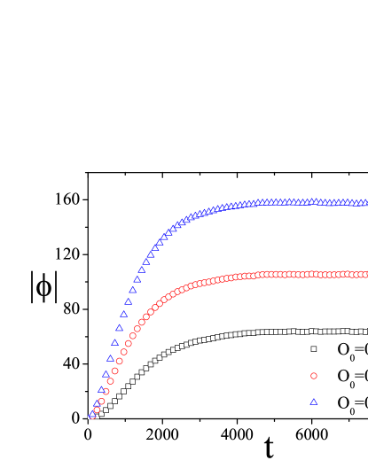
We can observe that increases with time, as Fig. 1. A convexity change is more sensitive to higher -values. The sum of these local variances corresponds to a part of , denoted by which was analytically obtained by Eq. 2.1. So we compute estimated by equation 2.1 which corresponds to the sum of all correlations of the payoffs until time , i.e., a kind of “cumulative” correlation.
In Fig. 2 we can check the behavior of . The points where , give , i.e, they work as a “decorrelation time” of the system that depends on initial offer . The points in Fig. 2 corresponds to MC simulations used to corroborate the results from equation 2.1. In this simulations we performed runs of the iterated game performing averages for each time. We can see a perfect agreement between Eq. 2.1 and MC simulations.
Now let us show the results for the reactive ultimatum game version when the acceptance depends on the offer and compare with the results of this subsection.
4.2 Mean-field for Acceptance Dependent on the Offer
We observed that reactive -fixed approach for acceptance of the offer leads to offers that increase or decrease along time. This is a possible behavior, but the experiments with human beings (see e.g. [5]) seem to avoid the undesirable situation leading to a fair steady state: fifty-fifty sharing.
The reactive ultimatum game, based on acceptances that depend on the offers produce a stable state independently of . This strong fixed point must be better understood. Here, the first question is to check the cumulative gain and variance of the offer for in this situation comparing these same values in the reactive -fixed game.
In Figure 3 (left plot) we show the temporal evolution of , i.e., the cumulative payoff up to time , according to Equation 2 for five -values. We can observe that case corresponds to the regime which changes with offer (10).
In the same Figure (right plot) we show the behavior of the variance of the payoff for the same -values (Eq. 2.1). The variance can increase or decrease, respectively, for and . For we have also the agreement with the case with dependent on the offer given by Equation 12
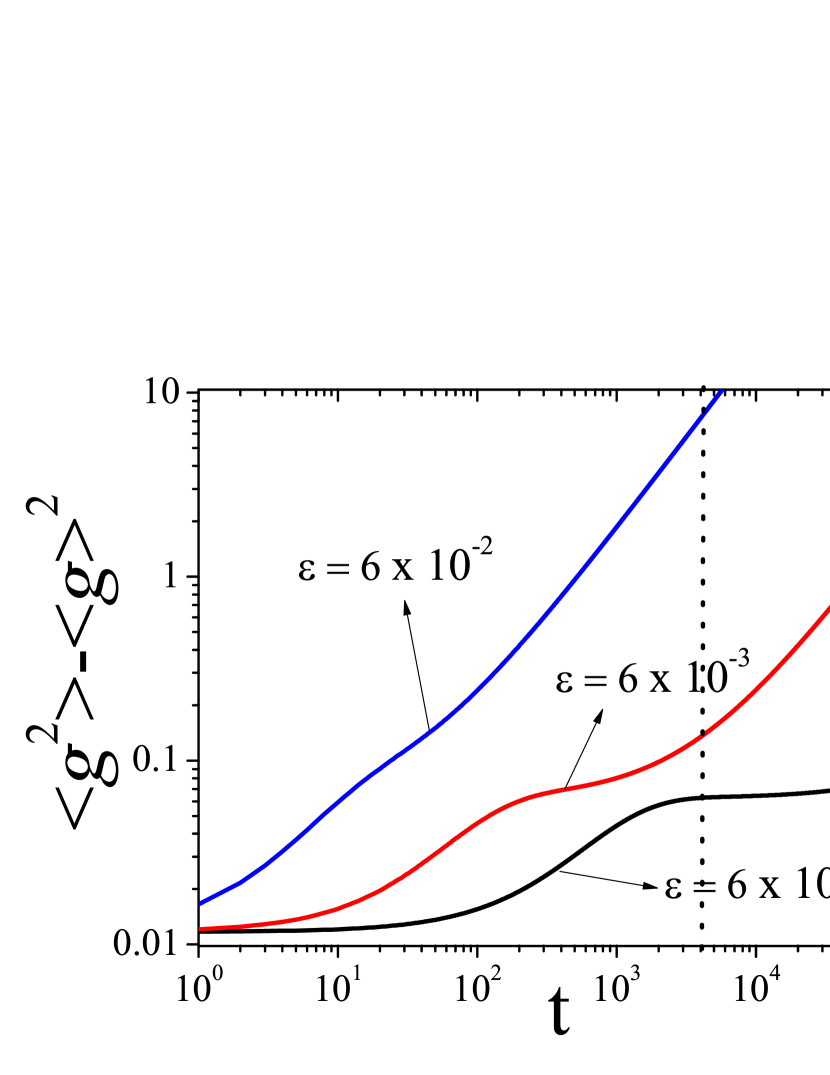
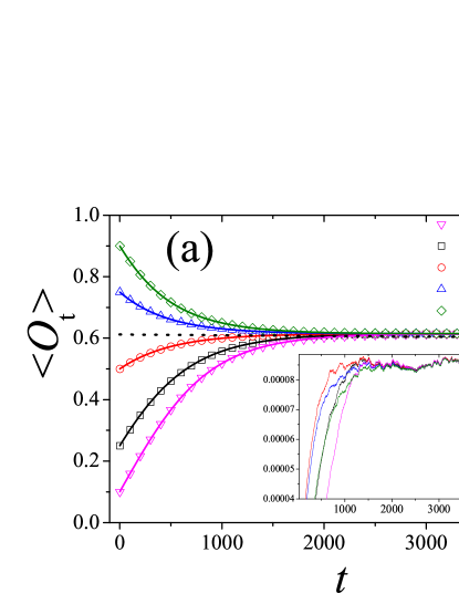
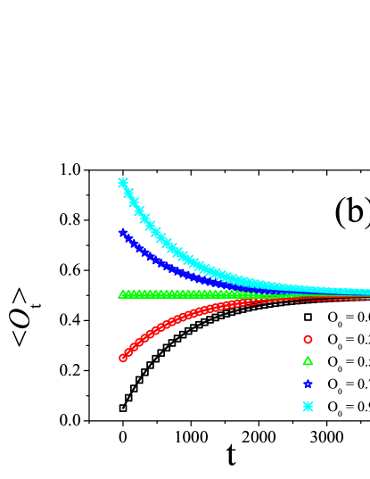
Now, it is interesting to observe what happens with other initial conditions for variance of payoff when the acceptance depends on the offer. We can observe in Fig. 4 that values of payoff dispersion always converge to the same value which does not depend on .

Particularly for , we observe that variance has a maximum before it converges to the steady state. This rich behavior is obviously related to the fact that on average that offer converges (see Eq. 9). In this same plot, we also show that MC simulations corroborate our analytical results.
So our reactive ultimatum game in mean field regime (two individuals iteratively playing) and with the values averaged for a huge number of repetitions (mean-field regime) is able to reproduce the intuitive aspect of the ultimatum game, which corroborates real situations.222As seen in this simple video: https://www.youtube.com/watch?v=YXfEv-xEWtE Finally looking at the variance of the cumulative payoff we can also estimate the value for this case as we performed for the -fixed approach.
In Fig. 5 (left) we show the variance of the cumulative payoff as a function of time which is only obtained by Monte Carlo simulations (full points). On the other hand, (lines), the sum of payoff variances for all times , were analytically estimated by Equations 13, 11, and 8.
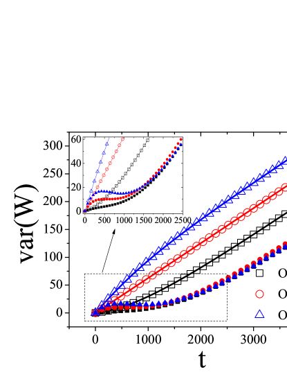
The empty points correspond to obtained by Monte Carlo simulations. By performing the difference we obtain . In Fig. 5 (right) we can observe that converges to a steady state well defined as the payoff and its variance. Remember that this is different for the -fixed approach (as seen in Fig. 2).
In summary, we observed that offer-dependent acceptance produces a fair steady state for these offers contrary to the expected rational behavior. But in this version of reactive ultimatum game other important questions can be answered: which are the effects of topologies, randomness, and the neighborhood size on the offers. In the next section (second part of our results) we analyze such effects on the reactive ultimatum game when the acceptance depends on the offer.
5 Results Part II: Coordination () and Randomness Effects ()
In this section we analyze the reactive ultimatum game in networks. We initially concentrate our attention for populations that play under policy I, in a regular graph with . In this case, we can set in equation 14, we have . For . We can iterate this equation. Simultaneously we have performed Monte Carlo simulations in a square lattice by considering that a player will make an offer to their four different neighbors and therefore will be the responder to another four different neighbors. The player changes her decision with respect to the offer only after having played with all neighbors, and the synchronous our asynchronous version of the MC simulations which are similar in this case.

Here an important question to ask is about the influence of randomness on these results. If we imagine for example a small world built from a simple ring or even a square lattice with coordination , by introducing a rewiring probability , we have but the result corresponds exactly, for example to policy I, by changing by corresponding ? This is not what happens. This occurs only if is large; for smaller we have a dependence on as can be observed in the color maps of Figure 7.
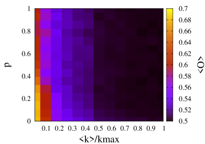
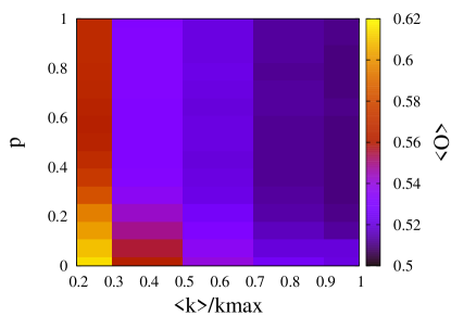
Such behavior can be checked by looking the dependence of stationary offer as function of and as shown in fig. 7. We performed simulations in a small world starting from a ring and a square lattice. It is interesting observe that for low coordination even for we do not obtain the result expected for mean field ().
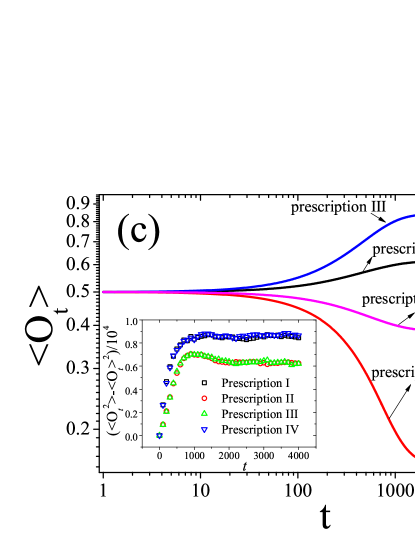
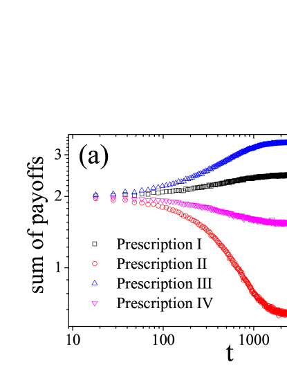
Now it is interesting to analyze the effects about the payoff of the players in populations under four different policies. We want to show the effects about distribution of payoff in populations as a function of time considering the populations in which the offers are performed under 4 different policies and acceptance occurs with probability exactly the offer of the player. We consider (). We can see from plot (C) in Fig. 6 that policy 3 leads to higher offers. This happens because players with this behavior only decrease their offers in really favorable situation; they prefer to deal with more players under lower offer values than playing with only one player under higher offer values. Bigger offers mean higher acceptance probabilities, which mean larger number of deals.
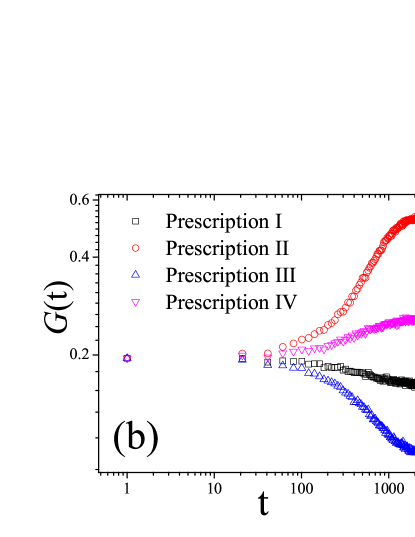
By considering the payoff obtained by players in populations interacting under the different policies, we analyzed statistics related to payoff obtained by the players in populations interacting under these different policies separately. We consider , for the sake of simplicity. One question to ask is how the payoff is distributed among the players along time. In this case, we can use a interesting concept from Economics, the Gini coefficient. Considering that players have their payoffs at time in increasing order: . So we consider the cumulative distribution:
The Lorentz () curve shows the corresponding wealth (sum of payoffs) corresponding to population fraction . We expect an identity function for a well distributed payoff. By a trapezoidal formula, the Gini coefficient can be estimated by
which measures the difference between the Lorentz curve and the identity function. This number changes from 0 up to 1, and the higher the value of , the worse is the payoff distribution.
Since we analyzed the properties of populations under different policies for , now we would like to better explore a general formula for the stationary offer for arbitrary coordination, considering populations under proportions of different policies. If we consider that , , and are the densities of conservative, greedy, highly conservative and moderated players, we can write that with the players inserted in a population with coordination , is
which results in
| (15) |
Obviously, Eq. 14 is a particular case of Eq. 15 (, ). So our work now is to change the proportions , , and , by numerically solving this equation and answering an important question: Is there some proportion that is able to change the behavior as ? First of all, it is important to mention that all results obtained by numerical integration of Eq. 15 were checked by performing simulations in rings and square lattices with arbitrary coordination. For this reason we will omit any information about MC simulations from that part until the final results, but remember that we have a perfect agreement between MC simulations and numerical integration of Eq. 15.
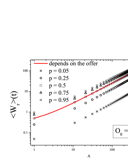
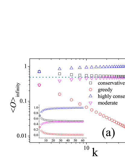
First, we would like to analyze the stationary average offer for mixing of different strategies, by looking at differences between the homogeneous populations (i.e., that one where players only use the same policy (I, II, III, or IV). In plot (a), Fig. 9, we show the behavior of as a function of in log-log scale. Each plot corresponds to one population interacting according to a specific policy (we denote it as homogeneous population). The inset plot corresponds to the same plot in linear scale. We can observe that in policies I and IV, the stationary offers converge to when , differently from II and III.
It is important to mention that a population with only greedy players leads to an algebraic decay of the offer as coordination (): . We measured the exponent by using and for which indicates a kind of hyperbolic scaling in coordination .
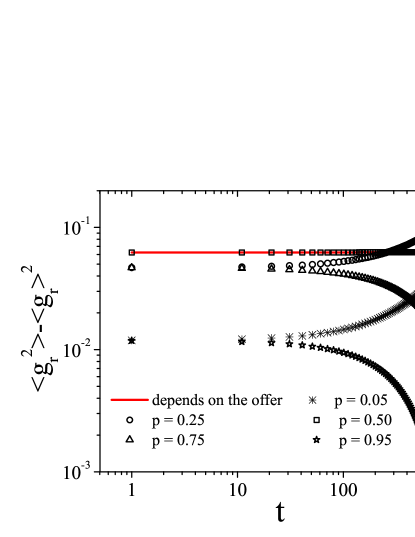
The first experiment with heterogeneous population keeps (. In this case, surprisingly the stationary case is independently from (by simplicity we omit this obvious plot). We cannot observe such behavior in the studied homogeneous populations.
Other exotic choices can be performed in which shows convex and concave behaviors as function of , i.e., with extrema well defined as we can observe in plot (b), Fig. 9.

6 Conclusions
In this paper we analyze some important aspects of populations which interact under a reactive ultimatum game. First we extended results of a recent publication where acceptance of the offers occurs with fixed probability . We show an interesting behavior for the sum of all temporal correlations of the payoff from : , which changes its signal in time that depends on the acceptance probability , that is a property from the fact that increases (respectively, decreases) as (resp.) as function of time.
Based on the fact that unfair offers have small acceptance probabilities, we proposed a new model where acceptance occurs with probability , i.e. the offer of the opponent. In this case a mean field regime leads to a interesting stationary fair offer: independently from the initial offer . Thus, the sum of the temporal correlations of the payoff has a steady state well defined, but depends on .
When studied in networks the model does not present for low coordination (small ) whatever the policy analyzed. Particularly for we showed that the average payoff is larger and the Gini coefficient is smaller for the policy that decreases the respective offer only when all players have accepted the offer at hand. This apparently altruistic player gains low values as proposer, but higher values as a responder; this combination leads to a well distributed payoff. We show that the absolutely greedy policy (II) leads to low payoffs and to high Gini coefficients.
Further, we introduced four policies that differ in how each player increases/decreases her offer. Only two policies present for . However a perfect equilibrium among policies, i.e. 1/4 of population for each policy, leads to independently from . There is a breaking of monotonicity of for mixing of strategies, which presents -values where is a extreme, either maximum or minimum value.
References
- [1] J. von Neumann, O. Morgenstern, ”Theory of Games and Economic Behavior” (Princeton University Press, Princeton NJ) (1944)
- [2] J. M. Smith, Journ. Theor. Biol. 47, 209-221 (1974)
- [3] G. Szabó, G. Fáth, Phys. Rep. 446, 97-216(2007)
- [4] W. Guth, R. Schmittberger and B. Schwarze, J. Econ. Behav. Org., 24, 153 (1982).
- [5] J. Henrich, Am. Econ. Rev. 90, 973 (2000)
- [6] A. Szolnoki, M. Perc, G. Szabó, Phys. Rev. Lett. 109, 078701-1 (2012).
- [7] A.G. Sanfey, J. K. Rilling, J.A. Aronson, L. E. Nystrom and J. D. Cohen, Science 300 1755 (2003).
- [8] T. C. Burnham, Proc. Royal Soc. B, 274, 2327-2330 (2007)
- [9] M. A. Nowak, K. M. Page, K. Sigmund, Science, 289 1773-1775 (2000).
- [10] E. Almeida, R. da Silva, A. S. Martinez, Physica A, 412, 54 (2014)
- [11] R. da Silva, G. A. Kellermann and L. C. Lamb, J. Theor. Biol., 258, 208-218 (2009).
- [12] R. da Silva and G. A. Kellerman, Braz. J. Phys., 37, 1206-1211 (2007).