A deconvolution path for mixtures
Abstract
We propose a class of estimators for deconvolution in mixture models based on a simple two-step “bin-and-smooth” procedure applied to histogram counts. The method is both statistically and computationally efficient: by exploiting recent advances in convex optimization, we are able to provide a full deconvolution path that shows the estimate for the mixing distribution across a range of plausible degrees of smoothness, at far less cost than a full Bayesian analysis. This enables practitioners to conduct a sensitivity analysis with minimal effort. This is especially important for applied data analysis, given the ill-posed nature of the deconvolution problem. Our results establish the favorable theoretical properties of our estimator and show that it offers state-of-the-art performance when compared to benchmark methods across a range of scenarios.
Key words: deconvolution, mixture models, penalized likelihood, empirical Bayes, sensitivity analysis
1 Deconvolution in mixture models
1.1 Introduction
Suppose that we observe from the model
| (1) |
where is a known distribution with location parameter , and is an unknown mixing distribution. Marginally, we have specified a mixture model for :
| (2) |
The problem of estimating the mixing distribution is commonly referred to as deconvolution: we observe draws from the convolution , rather than from directly, and we wish to invert this blur operation to recover the distribution of the latent location parameters. Models of this form have been used in a wide variety of applications and have attracted significant attention in the literature (e.g. Kiefer and Wolfowitz, 1956; Ferguson, 1973; Fan, 1991; Newton, 2002; Ghosal and Van Der Vaart, 2001). Yet the estimation of continues to pose both theoretical and practical challenges, making it an active area of statistical research (e.g. Delaigle and Hall, 2014; Efron, 2016).
In this paper, we propose a nonparametric method for deconvolution that is both statistically and computationally efficient. Our method can be motivated in terms of an underlying Bayesian model incorporating a prior into model (1), but it does not involve full Bayes analysis. Rather, we use a two-step “bin and smooth” procedure. In the “bin” step, we form a histogram of the sample, yielding the number of observations that fall into the th histogram bin. In the “smooth” step, we use the counts to compute a maximum a posteriori (MAP) estimate of under a prior that encourages smoothness.
We show that this nonparametric empirical-Bayes procedure yields excellent performance for deconvolution, at reduced computational cost compared to full nonparametric Bayesian methods. Our main theorems establish conditions under which the method yields a consistent estimate of the mixing distribution , and provide a concentration bound for recovery of the marginal distribution . We also provide simulation evidence that the method offers practical improvements over existing state-of-the-art methods.
2 Connections with previous work
We first recall the work by Kiefer and Wolfowitz (1956), who consider estimating using the nonparametric maximum likelihood estimation. The Kiefer–Wolfowitz estimator (KW) has some appealing features: it is completely nonparametric and invariant to translations of the data, it requires no tuning parameters, and it is consistent under fairly general conditions. Balanced against these desirable features there is, perhaps, a disadvantage when estimating a smooth true mixing density: the KW estimator is a discrete distribution involving as many as point masses.
Our approach to deconvolution falls within a penalized likelihood framework. It has important connections with classical ideas of penalized likelihood density estimation from Good and Gaskins (1971); Silverman (1982). And at least in spirit, our work resembles recent deconvolution methods by Lee et al. (2013); Wager (2013); Efron (2016). A detailed discussion or comparison between these methods and ours will be made in Section 5.
Deconvolution has also been studied using Bayesian methods. In the context of repeated measurements, or multivariate deconvolution, we highlight recent work by Sarkar et al. (2014a, b); Staudenmayer et al. (2008). Moreover, for the one dimensional density estimation problem, a flexible choice is the Dirichlet Process (DP) studied in Ferguson (1973) and Escobar and West (1995). For a Dirichlet prior in deconvolution problems, concentration rates were recently studied in Donnet et al. (2014). Related models were considered by Do et al. (2005) and Muralidharan (2010) for finite mixture of normals.
The DP provides a very general framework for estimating the mixing density . However, as Martin and Tokdar (2012) argue, fitting a Dirichlet process mixture does not scale well with the number of observations . For micro–array studies, ranges from thousands to tens of thousands, whereas for more recent studies of fMRI data or single-nucleotide polymorphisms, can reach several hundreds of thousands (e.g. Tansey et al., 2014). For such large data sets, fitting a DP mixture model can be very time-consuming.
To overcome this difficulty, Newton (2002), Tokdar et al. (2009), Martin and Tokdar (2011), and Martin and Tokdar (2012) studied a predictive recursive (PR) algorithm. The resulting estimator scales well with large data sets while remaining reasonably accurate, thereby solving one the main challenges faced by the fully Bayesian approach.
Finally, we note the work by Carroll and Hall (1988); Stefanski and Carroll (1990); Zhang (1990); Fan (1991); Fan and Koo (2002); Hall et al. (2007); Carroll et al. (2012); Delaigle and Hall (2014), among others, who considered kernel estimators. Their idea is motivated by (1) after taking the Fourier transform of the corresponding convolution of densities, then solving for the unknown mixing density using kernel approximations for the Fourier transform of the true marginal density. The resulting kernel estimator enjoys attractive theoretical properties: for each , the estimator has optimal rates of convergence towards for squared-error loss when the function belongs to a smooth class of functions (Fan, 1991).
3 A deconvolution path
3.1 Overview of approach
We now described our proposed approach in detail. We study deconvolution estimators related to the variational problem
| (3) |
where is a known penalty functional. The choices of we consider include or penalties on the derivatives in the log-space to encourage smoothness:
| (4) |
with or and where is the derivative of order of the log prior. The penalty involving the first derivative is an especially interpretable one, as is the score function of the mixing density.
Note that an alternative interpretation of our approach is as a MAP estimator. To see this we consider the (possibly improper) prior on the mixing density
where is an appropriate class of density functions. The posterior distribution is , and our MAP estimator therefore solves, for an appropriate ,
| (5) |
This belongs to a general class of MAP estimators that have been studied in Good and Gaskins (1971) and Silverman (1982) for the classical problem of density estimation. For deconvolution problems we note the recent work by Wager (2013) which penalizes the marginal density rather than the derivatives of the mixing density as we propose. Moreover such penalization is not motivated to encourage smoothness. Rather, it is an projection on to the space of acceptable marginal densities. An alternative penalized likelihood method was studied in Lee et al. (2013) in the different context where the marginal density has atoms. There the authors use the roughness penalty which differs from our approach that penalizes the log-mixing density and hence ensures that the solutions will be positive. Also, we allow different degrees of smoothness depending on the choice of . Moreover, while Lee et al. (2013) only considered sample sizes in the order of hundreds, we show in the next sections that our estimator can scale to much larger data sets while still enjoying attractive statistical properties.
More recently, Efron (2016) proposed a penalized approach to deconvolution that is also based on regularization but differs from ours. Such approach proceeds by assuming that the mixing density is discrete with support . Then Efron (2016) specified a parametric model on the mixing density of the form
where is the row of the matrix , for some , which is used to encourage structure on the mixing density. Moreover, is a normalizing constant satisfying
Then summing over all the and considering the contribution of the different samples, Efron (2016) arrives to the minus log-likelihood
The estimator from Efron (2016) results from solving
| (6) |
where is either or .
We note that the estimator (6) is possibly limited by the following aspects. First, the choice of the matrix , which Efron (2016) recommends to be a spline basis representation, might produce estimates that suffer from local adaptivity problems. Moreover, there is no theoretical support of choosing . In our experiments section we will present experimental comparisons between the estimator (6) and our approach.
Finally, we emphasize that our approach is not, in any sense, related to the ridge parameter deconvolution estimator from Hall et al. (2007). Such estimator does not penalizes that log-likelihood as we propose, but rather is designed to avoid the need to choose a kernel function, in the original kernel estimator from Fan (1991), by ridging the integral in its definition with a positive function.
3.2 Binned counts problem
Throughout this section we assume that corresponds to the pdf of the standard normal distribution, although the arguments can easily be generalized to other distributions.
To make estimation efficient in scenarios with thousands or even millions of observations, we actually fit a MAP estimator based on binning the data. First, we use the samples to form a histogram with bins, where is the th interval in the histogram and is the associated count. For ease of exposition, we assume that the intervals take the form , i.e. have midpoints and width , although this is not essential to our analysis. To arrive to a discrete estimator, instead of Problem (3), we consider an approximation, a reparametrization , and put the penalty in the objective function with a regulariation parameter ,
| (7) |
We then approximate (7) by solving
| (8) |
where or , and is the -th order discrete difference operator. Concretely, when , is the matrix encoding the first differences of adjacent values:
| (9) |
For , is defined recursively as , where from (9) is of the appropriate dimension. Thus when , we penalize the total variation of the vector (c.f. Rudin et al., 1992; Tibshirani et al., 2005) and should expect estimates that are shrunk towards piecewise-constant functions. When , the estimator penalizes higher-order versions of total variation, similar to the polynomial trend-filtering estimators studied by Tibshirani (2014).
3.3 Solution algorithms
We now discuss the implementation details for solving (10) in the case . To solve this problem, motivated by the work on trend filtering for regression by Ramdas and Tibshirani (2014), we rewrite the problem as
| (11) |
Next we proceed via the alternating-direction method of multipliers (ADMM), as in Ramdas and Tibshirani (2014). (See Boyd et al., 2011, for an overview of ADMM.) By exploiting standard results we arrive at the scaled augmented Lagrangian corresponding to the constrained problem (11):
This leads to the following ADMM updates at each iteration :
| (12) |
Note that in (12) the update for involves solving a sub-problem whose solution is not analytically available. To deal with this, we use the well known Broyden–Fletcher–Goldfarb–Shanno (BFGS) algorithm, which is very efficient because the gradient of the sub-problem objective is available in closed form. The update for can be computed in linear time by appealing to the dynamic programming algorithm from Johnson (2013).
In the case , both components of the objective function in (10) have closed-form gradients; see the appendix. Thus we can solve the problem using any algorithm that can use function and gradient calls. In particular, we use BFGS.
3.4 Solution path and model selection
One of the major advantages of our approach is that it easily yields an entire deconvolution path, comprising a family of estimates over a grid of smoothness parameters. Although in principle any deconvolution algorithm can yield such a path by solving the problem for many smoothing parameters, our path is generated in a highly efficient manner, using warm starts. We initially solve (11) for a large value of , for which the result estimate is nearly constant. We then use this solution to initialize the ADMM at a slightly smaller value of , which dramatically reduces the computation time compared to an arbitrarily chosen starting point. We proceed iteratively until solutions have been found across a decreasing grid of values (which are typically spaced uniformly in ).
The resulting deconvolution path can be used to inspect a range of plausible estimates for , with varying degrees of smoothness. This allows the data analyst to bring to bear any further prior information (such as the expected number of modes in ) that was not formally incorporated into the loss function. It also enables sensitivity analysis with respect to different plausible assumptions about the smoothness of the mixing distribution. We illustrate this approach with a real-data example in Section 4.
However, in certain cases—for example, in our simulation studies—it is necessary to select a particular value of using a default rule. We now briefly describe heuristics for doing so based on and penalties with . These heuristics are used in our simulation studies. For the case of regularization, motivated by Tibshirani and Taylor (2012), we consider a surrogate AIC approach by computing
and choosing the value of that minimizes this expression. Here, denotes the solution given by L1-D with regularization parameter .
In the case of regularization the situation is more difficult, since there is not an intuitive notion of the number of parameters of the model. Instead, we consider an ad-hoc procedure based on cross validation. This solves the problem for a grid of regularization parameters and chooses the parameter the minimizes , where is defined as
with the solution obtained by fitting the model on the training set which consists of of the data. Here, is evaluated using the counts from the held out set which has of the data, and is the number of observations in such set. Our motivation for using the additional term is that works well when the problem is formulated with regularization. However, when (10) is formulated using , the penalty is not suitable so instead we use . Our simulations in the experiments section will show that this rule works well in practice.
3.5 A toy example
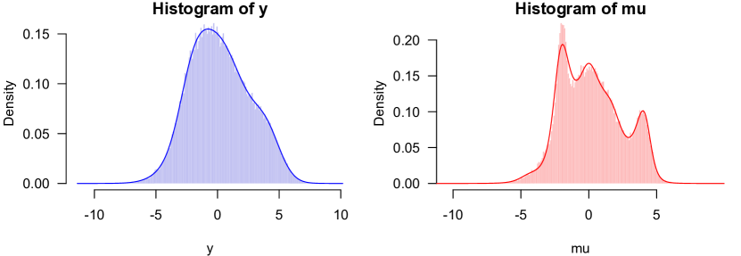
We conclude this section by illustrating the accuracy of our regularized deconvolution approach on a toy example. In this example we draw samples with the corresponding drawn from a mixture of three normal distributions. Figure 1 shows the samples of both the observations (left panel) and the means (right panel), together with the reconstructions provided by our method. Here, we solve the version of problem (10) by using the BFGS algorithm and choose using the heuristic just described.
It is clear that regularizing with an penalty provides an excellent fit of the marginal density. Surprisingly, it can also capture all three modes of the true mixing density, a feature which is completely obscured in the marginal). Our experiments in Section 6.1 will show in a more comprehensive way that our method far outperforms other approaches in its ability to provide accurate estimates for multi-modal mixing distributions.
4 Sensitivity analysis across the path
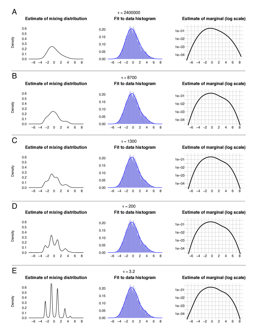

In this section, we provide an example of a sensitivity analysis using our deconvolution path estimator. We examine data originally collected and analyzed by Singh et al. (2002) on gene expression for 12,600 genes across two samples: 9 healthy patients and 25 patients with prostate tumors. The data come as a set of 12,600 -statistics computed from gene-by-gene tests for whether the mean gene-expression score differs between the two groups. After turning these 12,600 -statistics into -scores via a CDF transform, we estimate a deconvolution path assuming a Gaussian convolution kernel. We use an penalty and a grid of values evenly spaced on the logarithmic scale between and .
Each row of Figure 2 shows five points along the deconvolution path; the regularization parameter is largest in Row A and gets smaller in each successive row. Within each row, the left column shows the estimated mixing distribution for the given value of . The middle column shows the histogram of the data together with the fitted marginal density . The right column shows the fitted marginal density on the log scale, with a regular grid to facilitate comparison of the results across different values of .
The figure shows that, while the estimate of the mixing distribution changes dramatically across the deconvolution path, the estimate of the marginal density is much more stable. Even on the log scale (right column), the differences among the fitted marginal densities are not visually apparent in Panels B through E, even as the regularization parameter varies across three orders of magnitude.
This vividly demonstrates the well-known fact that deconvolution, especially of a Gaussian kernel, is a very ill-posed inverse problem. There is little information in the data to distinguish a smooth mixing distribution from a highly multimodal one, and the model-selection heuristics described earlier are imperfect. A decision to prefer Panel B to Panel E, for instance, is almost entirely due to the effect of the prior. Yet for most common deconvolution methods, the mapping between prior assumptions and the smoothness of the estimate is far from intuitive. By providing a full deconvolution path, our method makes this mapping visually explicit.
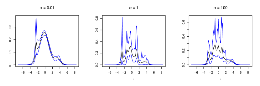
For reference, it is interesting to compare our deconvolution path to the results of other methods. Figure 3 shows the result of using MCMC to fit a 10-component mixture of normals to the mixing distribution. The weights in the Gaussian mixture were assigned three different symmetric Dirichlet priors, with concentration parameter . Panels 1-3 in Figure 3 show the posterior mean and posterior 95% credible envelopes for ; these settings span a wide range of expected degrees of smoothness for , and they yield a correspondingly wide range of posterior estimates. Comparing figures 2 and 3, we see that the deconvolution path spans essentially the entire range of plausible posterior estimates for arising under any of the concentration parameters. In contrast, Panels 4-7 in Figure show that the kernel estimates are either overly smooth or wiggly.
5 Theoretical properties
In this section we establish some important theoretical properties of our estimators by thinking of them as approximations to problems involving sieves. We start by showing consistency of the mixing density in L1 norm. We do not provide convergence rates since, unlike the kernel estimator from Fan (1991) and the predictive recursion from Newton (2002), our method cannot be expressed in analytical form. Moreover, while the method from Fan (1991) remarkably attains minimax rates under squared error loss for point estimates of the true mixing, in an earlier work Carroll and Hall (1988) suggested that convergence rates for Gaussian deconvolution might be too pessimistic given the unbounded support nature of the classes of functions considered. This is out of the scope of our paper, but we do provide evidence in the later sections that our estimator can outperform existing non-parametric methods.
Throughout we consider and to be fixed. We also denote by the set of densities in , thus , where denotes Lebesgue measure. Moreover, given any non-negative function we say that if
and is -Lipschitz. Here, given an arbitrary function , we use the notation to indicate the usual supremum norm on the support of . Moreover is called Lipschitz if it satisfies for all and .
In this section two metrics of interest will be repeatedly used. The first one is the usual distance . The other metric of interest will be the Hellinger distance whose square is given as . We also use the notation . Finally, for , we define the functional which will be a generalization of the usual total variation. We set .
Next we state some assumptions for our first consistency result. Our approach is to consider the objective function in (3) restricted to a smaller domain than that of its original formulation. This will then allows to prove that the new problem is not ill defined and also its solutions enjoy asymptotic properties of convergence towards the true mixing density. We refer to Geman and Hwang (1982) for a general perspective on sieves.
Assumptions and definitions
Let be a set of functions that satisfies the following.
Assumption 1.
Any function satisfies that , , , and there exists a constant .
Assumption 2.
For all , the exists a set and constants such that for all it holds that and . Moreover, for all , the set induces a tight set of of probability measures in satisfying . In addition, is dense in with respect to the metric .
Assumption 3.
Data model: we assume that are independent draws from the density , , with being an arbitrary density function satisfying and .
Assumption 4.
The set
satisfies for all , where the convergence is uniform in .
Assumption 5.
We assume that the are binned into different intervals with frequency counts such that , and we denote by an arbitrary point in interval . Note that this trivially holds for the case where and f for all .
Assumption 6.
There exists such that
If the and for all , this condition can be disregarded.
Assumptions (1)-(3) are natural for the original variational problem proposed earlier. The Lipschitz condition, the bounds on the behavior of the functions at zero, and the tightness of distributions are merely used to ensure that the sieves will indeed be compact sets with respect to the metric . Moreover, Assumption tell us that the sieves are rich enough to approximate the true mixing density sufficiently well. The last two assumptions can be disregarded when the counts in the bins are all one.
We are now ready to state our first consistency result. Its proof generalizes ideas from Theorem 1 in Geman and Hwang (1982).
Theorem 1.
If Assumptions (1-6) hold, then, the problem
has solution set . Moreover, for any sequence increasing slowly enough it holds that
In Theorem 1, the sequence is arbitrary and can grow as fast as desired. Moreover, the a.s statement is on the probability space with the measure on induced by , and with the completion of .
6 Experiments
6.1 Mixing density estimation
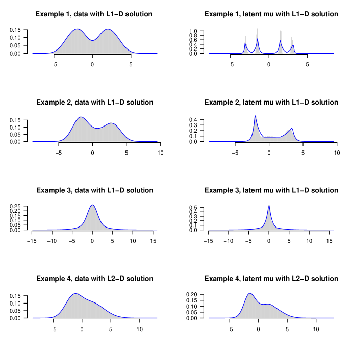
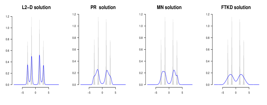
In this section we show the potential gain given by our penalized approaches. We start by considering the task of recovering the true mixing distribution. We evaluate the performance of our methods described in Section 3 which we call L1-deconvolution (L1-D) and L2-deconvolution (L2-D) depending on the regularization penalty used in the estimation. As competitors we consider a mixture of normals model (MN), the predictive recursion algorithm (PR) from Newton (2002), and the Fourier transform kernel deconvolution method (FTKD) from Fan (1991). Our comparisons are based on four examples which are shown in Figure 4. These examples are intended to illustrated the performance under different scenarios involving smooth and sharp densities. Next we describe the simulation setting and as well as the implementation details of the competing methods.
As a flexible Bayesian model we decided to use a prior for the mixing density based on a mixture of 10 normals (MN). Here, the weights of the mixture components are drawn from a Dirichlet prior with concentration parameter . This is done in order to have a uniform prior on the simplex. For the locations of the mixture we consider non-informative priors given as while for the variances of the mixture components we place a inverse gamma prior with shape parameter and rate . The complete model can be then thought as a weak limit approximation to the Dirichlet process, (Ishwaran and Zarepour, 2002). Also, Gibss sampling is accomplished straightforwardly by introducing a data augmentation with a variable indicating the component to which belong.
The next competing model is the predictive recursion algorithm from Newton (2002) for which we choose the weights as in Martin and Tokdar (2012), close to the limit of the upper bound of the convergence rate for PR given in Tokdar et al. (2009). Moreover we average the PR estimator over different permutations of the input data in order to obtain a smaller expected error Tokdar et al. (2009).
On the other hand, for the Fourier transform kernel deconvolution method, we consider different choices of bandwidth: the rule of thumb from Fan (1991), the plug in bandwidth from Stefanski and Carroll (1990), and the 2-stage plug-in bandwidth from Delaigle and Gijbels (2002). Our estimates are obtained using the R package fDKDE available at http://www.ms.unimelb.edu.au/~aurored/links.html, which addresses the main concerns associated with the R package decon, see Delaigle (2014).
For the final competitor, the “g-modeling” approach from Efron (2016) (g-M), we use the newly released R package deconvolveR.
| n | ||||||||||||
|---|---|---|---|---|---|---|---|---|---|---|---|---|
| 2000 | 9.47 | 9.12 | 9.39 | 9.69 | 8.89 | 9.27 | 9.26 | 8.91 | 9.18 | 9.48 | 8.89 | 9.01 |
| 10000 | 8.43 | 8.72 | 8.64 | 7.44 | 8.87 | 9.22 | 8.24 | 8.52 | 8.44 | 7.28 | 8.87 | 9.00 |
| 25000 | 8.34 | 8.46 | 7.27 | 5.54 | 8.88 | 9.32 | 8.15 | 8.27 | 7.13 | 5.43 | 8.16 | 9.09 |
| 50000 | 8.21 | 8.23 | 5.80 | 4.15 | 8.85 | 9.40 | 8.03 | 8.04 | 5.71 | 4.09 | 8.66 | 9.18 |
| 100000 | 8.34 | 8.05 | 4.79 | 3.38 | 8.69 | 9.50 | 8.14 | 7.86 | 4.69 | 3.35 | 8.49 | 9.28 |
We now state the simulation setting for recovering the mixing density. Given the densities from Figure 4, we consider varying the number of samples and for each fixed we run 100 Monte Carlo simulations. Moreover, for our methods we set , the number of evenly space points in the grid, to 250. See the appendix for a sensitivity example of this parameter.
The results on Table 1 illustrate a clear advantage of our penalized likelihood approaches over MN, PR and FTKD which seems even more significant for larger samples size. The estimated mixing density by L1-D is shown in Figure 4 where we can clearly see that L1-D can capture the peaks of the unknown mixing density. Moreover, Figure 5 shows that L2-D can also capture the structure of the true density. In contrast, MN, PR and FTKD all fail to provide reliable estimators.
| n | ||||||||||||
|---|---|---|---|---|---|---|---|---|---|---|---|---|
| 2000 | 6.20 | 2.54 | 2.74 | 2.38 | 6.07 | 8.23 | 5.47 | 2.37 | 2.49 | 2.13 | 5.86 | 7.06 |
| 10000 | 3.45 | 1.75 | 1.60 | 1.68 | 5.98 | 5.82 | 3.05 | 1.60 | 1.46 | 1.49 | 5.76 | 5.45 |
| 25000 | 2.31 | 1.46 | 1.19 | 1.35 | 5.99 | 5.01 | 2.20 | 1.35 | 1.09 | 1.19 | 5.70 | 4.77 |
| 50000 | 1.24 | 1.28 | 0.89 | 1.18 | 5.89 | 4.68 | 1.10 | 1.17 | 0.81 | 1.05 | 5.66 | 4.39 |
| 100000 | 0.78 | 1.07 | 0.74 | 0.87 | 4.97 | 4.03 | 0.69 | 0.98 | 0.67 | 0.77 | 4.85 | 3.85 |
| n | ||||||||||||
|---|---|---|---|---|---|---|---|---|---|---|---|---|
| 2000 | 5.28 | 1.83 | 2.09 | 0.96 | 4.95 | 7.16 | 3.45 | 1.21 | 1.37 | 0.63 | 3.25 | 4.54 |
| 10000 | 3.06 | 1.38 | 1.46 | 0.61 | 4.86 | 1.45 | 1.99 | 0.90 | 0.95 | 0.40 | 3.18 | 9.49 |
| 25000 | 1.51 | 1.16 | 1.18 | 0.47 | 4.61 | 1.18 | 0.99 | 0.72 | 0.77 | 0.31 | 3.01 | 7.75 |
| 50000 | 0.95 | 1.06 | 1.00 | 0.42 | 3.77 | 1.13 | 0.62 | 0.70 | 0.66 | 0.28 | 2.47 | 9.11 |
| 100000 | 0.72 | 0.95 | 0.86 | 0.38 | 3.48 | 2.42 | 0.47 | 0.62 | 0.56 | 0.25 | 2.29 | 1.58 |
| n | ||||||||||||
|---|---|---|---|---|---|---|---|---|---|---|---|---|
| 2000 | 20.6 | 4.75 | 1.82 | 3.48 | 3.25 | 7.06 | 16.8 | 4.03 | 1.15 | 2.88 | 3.00 | 5.88 |
| 10000 | 7.64 | 1.89 | 0.65 | 1.93 | 2.87 | 4.20 | 6.23 | 1.60 | 0.53 | 1.60 | 2.67 | 3.53 |
| 25000 | 2.04 | 1.10 | 0.48 | 2.19 | 2.57 | 2.34 | 1.67 | 0.93 | 0.39 | 1.80 | 2.37 | 1.95 |
| 50000 | 1.03 | 0.69 | 0.36 | 1.20 | 2.02 | 1.95 | 0.85 | 0.58 | 0.30 | 1.00 | 1.86 | 1.62 |
| 100000 | 0.50 | 0.55 | 0.39 | 0.90 | 1.36 | 1.49 | 0.40 | 0.46 | 0.32 | 0.85 | 1.25 | 1.22 |
For our example density 2, we observe from Table 2 that in general L2-D and L1-D offer the best performance. In the case of example 3, we observe that the L1-D again provides better results than the competitors in all the scenarios of sample sizes considered. Even with only 10000 samples L1-D is closer to the true density than all the other methods with more samples. Moreover, L2-D performs much better than PR and FTKD. Also, L2-D seems to be a clear competitor to MN. In the final example density 4, we observe that L2-D is the best method in all the scenarios considered.
Overall, we have shown that for estimating the mixing density, L1-D and L2-D can perform well under different settings, even when other methods exhibit notable deficiencies. The advantage is amplified by the fact that both of our methods are less computationally intensive that MN, with L2-D requiring around 40 seconds to handle problems with , and L1-D under the same problem conditions typically requires around 5 minutes for a full solution path across 50 values of the tuning parameter.
6.2 Normal means estimation
After evaluating our proposed methodology for the task of estimating the mixing density, we now, for the case of standard normal kernel, focus on the estimation of the normals means . For this, we consider comparisons using the best four among the methods used before in addition to other procedures that we briefly discuss next.
As it is well known (e.g Efron (2011) for description and references ), assuming that the marginal density is known, one can use Tweedie’s formula to estimate . For all the methods here this is the approach that we take, except for MN in which case we use the posterior means resulting from Gibss sampling inference. For the methods depending on grid estimator, the number of bins is set to .
For the method of Efron (2011), we set to 5 the degree of the polynomial approximation to the logarithm of the marginal true density (we found larger values to be less numerically stable). The Poisson surrogate model is then fit in R using the command glm. We also compare against the general maximum likelihood empirical-Bayes estimator (GMLEB) from Jiang and Zhang (2009), which is a discretized version of the original Kiefer–Wolfowitz estimator. For our comparisons we use the algorithm proposed in Koenker and Mizera (2014) based on an interior point method algorithm (GMLEBIP). We use the R package REBayes in order to obtain this estimator (Koenker (2013)). On the other hand, for the shape constrained (SC) estimator from Koenker and Mizera (2014), we rely on a binned count approach based on a weighted likelihood using R code provided by the authors. Moreover, we consider the estimator from Brown and Greenshtein (2009) using the default choice of bandwidth , which we refer to as BG. The finally competitor is the non-linear projection (NLP) estimator from Wager (2013).
| n | L2-D | L1-D | PR | MN | Efron | GMLEBIP | SC | BG | NLP |
| 2000 | 64.31 | 64.29 | 64.16 | 67.50 | 70.27 | 64.48 | 68.24 | 65.57 | 64.11 |
| 10000 | 63.89 | 63.68 | 63.86 | 63.18 | 70.00 | 63.80 | 65.56 | 64.06 | 63.27 |
| 25000 | 63.52 | 63.37 | 63.69 | 63.84 | 69.96 | 63.39 | 64.66 | 63.65 | 63.60 |
| 50000 | 63.27 | 63.21 | 63.55 | 65.20 | 69.85 | 63.23 | 64.15 | 63.44 | 63.26 |
| 100000 | 63.27 | 63.23 | 63.59 | 63.79 | 69.89 | 63.21 | 63.86 | 63.39 | 63.18 |
From Table 3 it is clear that the best methods for example 1 are L1-D, L2-D, GMLEBIP, and NLP. Moreover, it is not surprising that GMLEBIP provides good estimates given that the true mixing density has mixture components that have small variance.
For example 2, we can see from Table 4 that again L2-D and L1-D provide competitive estimates. The other suitable methods for this example seem to be PR and GMLEBIP. With slightly worse estimates MN, BG and SC provide results that are still competitive, with SC being particularly attractive given its computational speed to provide solutions.
| n | L2-D | L1-D | PR | MN | Efron | GMLEBIP | SC | BG | NLP |
| 2000 | 65.42 | 65.46 | 65.36 | 64.33 | 69.97 | 66.20 | 69.60 | 66.99 | 65.75 |
| 10000 | 64.98 | 65.06 | 65.08 | 65.66 | 69.75 | 65.29 | 67.10 | 65.54 | 65.95 |
| 25000 | 65.19 | 65.08 | 65.32 | 65.21 | 69.94 | 65.12 | 66.42 | 65.49 | 65.09 |
| 50000 | 64.99 | 65.08 | 65.13 | 65.44 | 69.93 | 65.03 | 65.97 | 65.19 | 65.24 |
| 100000 | 65.02 | 64.95 | 65.14 | 65.03 | 69.84 | 65.02 | 65.69 | 65.14 | 64.96 |
| n | L2-D | L1-D | PR | MN | Efron | GMLEBIP | SC | BG | NLP |
| 2000 | 64.99 | 64.96 | 65.41 | 69.05 | 70.54 | 65.74 | 69.70 | 66.99 | 65.77 |
| 10000 | 64.73 | 64.76 | 64.96 | 64.21 | 71.34 | 64.85 | 66.92 | 65.36 | 64.81 |
| 25000 | 64.52 | 64.57 | 64.75 | 64.97 | 71.42 | 64.65 | 66.62 | 64.82 | 64.62 |
| 50000 | 64.51 | 64.61 | 64.73 | 65.38 | 71.52 | 64.64 | 66.60 | 64.67 | 64.57 |
| 100000 | 64.54 | 64.41 | 64.76 | 64.54 | 71.96 | 64.56 | 65.17 | 64.62 | 64.46 |
| n | L2-D | L1-D | PR | MN | Efron | GMLEBIP | SC | BG | NLP |
| 2000 | 79.63 | 80.20 | 79.89 | 78.68 | 80.00 | 80.97 | 85.47 | 81.58 | 80.01 |
| 10000 | 79.32 | 79.35 | 79.42 | 79.34 | 79.99 | 79.74 | 82.18 | 79.89 | 79.64 |
| 25000 | 79.39 | 79.31 | 79.48 | 78.79 | 79.96 | 79.30 | 80.98 | 79.65 | 79.39 |
| 50000 | 79.21 | 79.25 | 79.29 | 79.85 | 79.82 | 79.40 | 80.58 | 79.36 | 79.39 |
| 100000 | 79.29 | 79.22 | 79.37 | 79.51 | 79.91 | 79.30 | 80.15 | 79.37 | 79.36 |
Finally, for examples 3 and 4 we can see in Tables 5 and 6 respectively that L1-D and L2-D are the best or among the best methods in terms of mean squared distance when recovering the unknown means . Table 6 also suggests that Efron’s estimator is more suitable when the true mixing density is very smooth with no sharp peaks.
7 Discussion
In many problems in statistics and machine learning, we observe a blurred version of an unknown mixture distribution which we would like to recover via deconvolution. The main challenge is to find an approach that is computationally fast but still possesses nice statistical guarantees in the form of rates of convergence. We propose a two-step “bin-and-smooth” procedure that achieves both of these goals. This reduces the deconvolution problem to a Poisson-regularized model would can be solved either via standard methods for smooth optimization, or with a fast version of the alternating-direction method of multipliers (ADMM). Our approach reduces the computational cost compared to a fully Bayesian method and yields a full deconvolution path to illustrate the sensitivity of our solution to the specification of the amount of regularization. We provide theoretical guarantees for our procedure. In particular, under suitable regularity conditions, we establish the almost-sure convergence of our estimator towards the mixing density.
There are a number of directions for future inquiry, including multivariate extensions and extensions to multiple hypothesis testing. These are active areas of current research.
References
- Boyd et al. (2011) S. Boyd, N. Parikh, E. Chu, B. Peleato, and J. Eckstein. Distributed optimization and statistical learning via the alternating direction method of multipliers. Foundations and Trends® in Machine Learning, 3(1):1–122, 2011.
- Brown and Greenshtein (2009) L. D. Brown and E. Greenshtein. Nonparametric empirical bayes and compound decision approaches to estimation of a high-dimensional vector of normal means. The Annals of Statistics, pages 1685–1704, 2009.
- Carroll et al. (2012) R. Carroll, A. Delaigle, and P. Hall. Deconvolution when classifying noisy data involving transformations. Journal of the American Statistical Association, 107(499):1166–1177, 2012.
- Carroll and Hall (1988) R. J. Carroll and P. Hall. Optimal rates of convergence for deconvolving a density. Journal of the American Statistical Association, 83(404):1184–1186, 1988.
- Delaigle (2014) A. Delaigle. Nonparametric kernel methods with errors-in-variables: Constructing estimators, computing them, and avoiding common mistakes. Australian & New Zealand Journal of Statistics, 56(2):105–124, 2014.
- Delaigle and Gijbels (2002) A. Delaigle and I. Gijbels. Estimation of integrated squared density derivatives from a contaminated sample. Journal of the Royal Statistical Society: Series B (Statistical Methodology), 64(4):869–886, 2002.
- Delaigle and Hall (2014) A. Delaigle and P. Hall. Parametrically assisted nonparametric estimation of a density in the deconvolution problem. Journal of the American Statistical Association, 109(506):717–729, 2014.
- Do et al. (2005) K.-A. Do, P. Muller, and F. Tang. A Bayesian mixture model for differential gene expression. Journal of the Royal Statistical Society, Series C, 54(3):627–44, 2005.
- Donnet et al. (2014) S. Donnet, V. Rivoirard, J. Rousseau, and C. Scricciolo. Posterior concentration rates for empirical bayes procedures, with applications to dirichlet process mixtures. arXiv preprint arXiv:1406.4406, 2014.
- Efron (2011) B. Efron. Tweedie’s formula and selection bias. Journal of the American Statistical Association, 106(496):1602–14, 2011.
- Efron (2016) B. Efron. Empirical bayes deconvolution estimates. Biometrika, 103(1):1–20, 2016.
- Escobar and West (1995) M. D. Escobar and M. West. Bayesian density estimation and inference using mixtures. Journal of the American Statistical Association, 90:577–88, 1995.
- Fan (1991) J. Fan. On the optimal rates of convergence for nonparametric deconvolution problems. The Annals of Statistics, pages 1257–1272, 1991.
- Fan and Koo (2002) J. Fan and J.-Y. Koo. Wavelet deconvolution. Information Theory, IEEE Transactions on, 48(3):734–747, 2002.
- Ferguson (1973) T. S. Ferguson. A Bayesian analysis of some nonparametric problems. The Annals of Statistics, 1:209–30, 1973.
- Geman and Hwang (1982) S. Geman and C.-R. Hwang. Nonparametric maximum likelihood estimation by the method of sieves. The Annals of Statistics, 10(2):401–14, 1982.
- Ghosal and Van Der Vaart (2001) S. Ghosal and A. W. Van Der Vaart. Entropies and rates of convergence for maximum likelihood and bayes estimation for mixtures of normal densities. The Annals of Statistics, pages 1233–1263, 2001.
- Good and Gaskins (1971) I. J. Good and R. A. Gaskins. Nonparametric roughness penalties for probability densities. Biometrika, 58(2):255–77, 1971.
- Hall et al. (2007) P. Hall, A. Meister, et al. A ridge-parameter approach to deconvolution. The Annals of Statistics, 35(4):1535–1558, 2007.
- Ishwaran and Zarepour (2002) H. Ishwaran and M. Zarepour. Exact and approximate sum representations for the dirichlet process. The Canadian Journal of Statistics/La Revue Canadienne de Statistique, pages 269–283, 2002.
- Jiang and Zhang (2009) W. Jiang and C.-H. Zhang. General maximum likelihood empirical bayes estimation of normal means. The Annals of Statistics, 37(4):1647–1684, 2009.
- Johnson (2013) N. A. Johnson. A dynamic programming algorithm for the fused lasso and l 0-segmentation. Journal of Computational and Graphical Statistics, 22(2):246–260, 2013.
- Kiefer and Wolfowitz (1956) J. Kiefer and J. Wolfowitz. Consistency of the maximum likelihood estimator in the presence of infinitely many incidental parameters. The Annals of Mathematical Statistics, 27:887–906, 1956.
- Koenker (2013) R. Koenker. Rebayes: empirical bayes estimation and inference in r. R package version 0.41, 2013.
- Koenker and Mizera (2014) R. Koenker and I. Mizera. Convex optimization, shape constraints, compound decisions, and empirical bayes rules. Journal of the American Statistical Association, 109(506):674–685, 2014.
- Lee et al. (2013) M. Lee, P. Hall, H. Shen, J. S. Marron, J. Tolle, and C. Burch. Deconvolution estimation of mixture distributions with boundaries. Electronic journal of statistics, 7:323, 2013.
- Martin and Tokdar (2011) R. Martin and S. T. Tokdar. Semiparametric inference in mixture models with predictive recursion marginal likelihood. Biometrika, 98(3):567–582, 2011.
- Martin and Tokdar (2012) R. Martin and S. T. Tokdar. A nonparametric empirical Bayes framework for large-scale multiple testing. Biostatistics, 13(3):427–39, 2012.
- Muralidharan (2010) O. Muralidharan. An empirical bayes mixture method for effect size and false discovery rate estimation. The Annals of Applied Statistics, pages 422–438, 2010.
- Newton (2002) M. A. Newton. On a nonparametric recursive estimator of the mixing distribution. Sankhyā: The Indian Journal of Statistics, Series A, pages 306–322, 2002.
- Padilla and Scott (2015) O. H. M. Padilla and J. G. Scott. Nonparametric density estimation by histogram trend filtering. arXiv preprint arXiv:1509.04348, 2015.
- Ramdas and Tibshirani (2014) A. Ramdas and R. J. Tibshirani. Fast and flexible ADMM algorithms for trend filtering. Technical report, Carnegie Mellon University, http://www.stat.cmu.edu/ ryantibs/papers/fasttf.pdf, 2014.
- Rudin et al. (1992) L. Rudin, S. Osher, and E. Faterni. Nonlinear total variation based noise removal algorithms. Physica D: Nonlinear Phenomena, 60(259–68), 1992.
- Sarkar et al. (2014a) A. Sarkar, B. K. Mallick, J. Staudenmayer, D. Pati, and R. J. Carroll. Bayesian semiparametric density deconvolution in the presence of conditionally heteroscedastic measurement errors. Journal of Computational and Graphical Statistics, 23(4):1101–1125, 2014a.
- Sarkar et al. (2014b) A. Sarkar, D. Pati, B. K. Mallick, and R. J. Carroll. Bayesian semiparametric multivariate density deconvolution. arXiv preprint arXiv:1404.6462, 2014b.
- Silverman (1982) B. W. Silverman. On the estimation of a probability density function by the maximum penalized likelihood method. The Annals of Statistics, pages 795–810, 1982.
- Singh et al. (2002) D. Singh, P. G. Febbo, K. Ross, D. G. Jackson, J. Manola, C. Ladd, P. Tamayo, A. A. Renshaw, A. V. D’Amico, J. P. Richie, E. S. Lander, M. Loda, P. W. Kantoff, T. R. Golub, and W. R. Sellers. Gene expression correlates of clinical prostate cancer behavior. Cancer Cell, 1(2):203–9, 2002.
- Staudenmayer et al. (2008) J. Staudenmayer, D. Ruppert, and J. P. Buonaccorsi. Density estimation in the presence of heteroscedastic measurement error. Journal of the American Statistical Association, 103(482):726–736, 2008.
- Stefanski and Carroll (1990) L. A. Stefanski and R. J. Carroll. Deconvolving kernel density estimators. Statistics, 21(2):169–184, 1990.
- Tansey et al. (2014) W. Tansey, O. Koyejo, R. A. Poldrack, and J. G. Scott. False discovery rate smoothing. Technical report, University of Texas at Austin, 2014. http://arxiv.org/abs/1411.6144.
- Tibshirani et al. (2005) R. Tibshirani, M. Saunders, S. Rosset, J. Zhu, and K. Knight. Sparsity and smoothness via the fused lasso. Journal of the Royal Statistical Society (Series B), 67:91–108, 2005.
- Tibshirani (2014) R. J. Tibshirani. Adaptive piecewise polynomial estimation via trend filtering. The Annals of Statistics, 42(1):285–323, 2014.
- Tibshirani and Taylor (2012) R. J. Tibshirani and J. Taylor. Degrees of freedom in lasso problems. The Annals of Statistics, 40(2):1198–1232, 2012.
- Tokdar et al. (2009) S. T. Tokdar, R. Martin, and J. K. Ghosh. Consistency of a recursive estimate of mixing distributions. The Annals of Statistics, pages 2502–2522, 2009.
- Wager (2013) S. Wager. A geometric approach to density estimation with additive noise. Statistica Sinica, 2013.
- Wald (1949) A. Wald. Note on the consistency of the maximum likelihood estimate. The Annals of Mathematical Statistics, pages 595–601, 1949.
- Zhang (1990) C.-H. Zhang. Fourier methods for estimating mixing densities and distributions. The Annals of Statistics, pages 806–831, 1990.
Appendix A Technical supplement
A.1 Gradient expression for regularization
Here we write the mathematical expressions for the gradient of the objective function when performing L2 deconvolution, As in Section 3.3 of the main document. Using the notation there, we have that
and
A.2 Proof of Theorem 1
Proof.
Motivated by Geman and Hwang (1982), given we define the function for . Clearly, is a density that induces a measure in that is absolutely continuous with respect to the Lebesgue measure in . Also, we observe that if , then, for any Borel measurable set , we have by Tonelli’s theorem that
Hence implies that and induce the same probability measures in .
Next we verify the assumptions in Theorem 1 from Geman and Hwang (1982). This is done into different steps below. Steps 1-4 verify the assumptions B1-B4 in Theorem 1 from Geman and Hwang (1982). Steps 5-6 are needed in the general case in which the data is binned. These are also related to ideas from Wald (1949).
1
Given and , the function
is continuous and therefore measurable on . To see this, simply note that for any we have that
Hence all the functions are -Lipschitz and the claim follows. Also, we note that
This follows by noticing that
2
Define for any function . Then for any and we have
3
Next we show that is compact on . Throughout, we use the notation to indicate uniform convergence. To show the claim, choose a sequence in . Then since are Lipschitz and uniformly bounded it follows by Arzela-Ascoli Theorem that there exists a sub-sequence such that in for some function which is also Lipschitz. Note that we can again use Arzela-Ascoli Theorem applied to the sequence to ensure that there exists a sub-sequence such that in . Thus we extend the domain of if necessary.
Proceeding by induction we conclude that for every there exists a sequence such that
in as . Hence with Cantor’s diagonal argument we conclude that there exists a sub-sequence such that
in for all . Since for all . Then without loss of generality, we can assume that
in for all and where the function satisfies . Continuing with this process we can assume, without loss of generality, that
in for all for some function satisfying for all . Therefore,
| (13) |
in for all .
Let us now prove that . First, we observe by the Fatou’s lemma is integrable in with respect to the Lebesgue measure. since is tight and, we obtain
This clearly also implies that integrates to or . Note that also by Fatou’s lemma we have that and by construction,
Finally, combining all of this with being -Lipschitz, we arrive to .
4 By assumption (4), we have that
5
Let us show that
for all . First, note that for all
Hence, by Step 1 we obtain
Now we observe that
and the claim follows from the monotone convergence theorem.
If and for all , the claim of Theorem 1 follows from Theorem 1 from Geman and Hwang (1982). Otherwise, we continue the proof below. In either case we can see that the solution set is not empty given that the map is continuous with respect to the metric for any .
6
Note that, by Glivenko-Cantelli Theorem and our assumption on the maximum number of bins, we have that, almost surely, the random distribution
converges weakly to the distribution function associated with . Hence, almost surely, from the Portmanteau theorem we have for any and any it holds that
| (14) |
since the function
is continuous and bounded by above.
Next we define
Clearly, implies . Also, we see that the set is d-compact. Hence, there exists in such that for positive constants satisfying that
for . Therefore from our assumptions on the sets and also from (14), we arrive at
Hence
This implies
Next we define
and we set . Therefore,
Next we define as
Then, implies . We also see that is d-compact. Hence there exists in such that for positive constants satisfying
for . Therefore,
So proceeding as before we obtain
Finally we define
and we set for all and . By construction, we have that
Thus an induction argument allow us to conclude the proof.
∎
Appendix B Simulation details
For the cases of the true mixing density we consider four densities of the form
In all cases considered here, the observations arise as in (1) with a standard normal sampling model. In our first example we evaluate performance for samples of a density that has four peaks or explicitly , , and with small variance . For the second example we consider a mixture of three normals two of which are smooth while the other has a peak. The true parameters in this case are , , and . The next example is a mixture of normals, one of which has very high variance. The true parameters chosen are , and . Our final example is a mixture, with , giving raise to a very smooth density, the parameters are , and . A visualization of these examples is shown in Figure 4.
B.1 Sensitivity to the number of bins

Figure 6 shows the performance of both L1-D and L2-D generally improves as we increase . However, based on our experience, is a reasonable choice. Specially for L1-D whose computational burden increases more rapidly. For it typically takes around min to compute the solution path for L1-D with 50 values of the regularization parameter. In contrast, L2-D only requires around 40 seconds under the same setting.