Data-Dependent Path Normalization
in Neural Networks

Abstract

We propose a unified framework for neural net normalization, regularization and optimization, which includes Path-SGD and Batch-Normalization and interpolates between them across two different dimensions. Through this framework we investigate the issue of invariance of the optimization, data dependence and the connection with natural gradients.

1 Introduction

The choice of optimization method for non-convex, over-parametrized models such as feed-forward neural networks is crucial to the success of learning—not only does it affect the runtime until convergence, but it also effects which minimum (or potentially local minimum) we will converge to, and thus the generalization ability of the resulting model. Optimization methods are inherently tied to a choice of geometry over parameter space, which in turns induces a geometry over model space, which plays an important role in regularization and generalization (Neyshabur et al., 2015c).

In this paper, we focus on two efficient alternative optimization approaches proposed recently for feed-forward neural networks that are based on intuitions about parametrization, normalization and the geometry of parameter space: Path-SGD (Neyshabur et al., 2015a) was derived as steepest descent algorithm with respect to particular regularizer (the $\ell_{2}$-path regularizer, i.e. the sum over all paths in the network of the squared product over all weights in the path  (Neyshabur et al., 2015b)) and is invariant to weight reparametrization. Batch-normalization (Ioffe & Szegedy, 2015) was derived by adding normalization layers in the network as a way of controlling the variance of the input each unit receives in a data-dependent fashion. In this paper, we propose a unified framework which includes both approaches, and allows us to obtain additional methods which interpolate between them. Using our unified framework, we can also tease apart and combine two different aspects of these two approaches: data-dependence and invariance to weight reparametrization.

Our unified framework is based on first choosing a per-node complexity measure we refer to as $\gamma_{v}$ (defined in Section 3). The choice of complexity measure is parametrized by a choice of “normalization matrix” $R$, and different choices for this matrix incorporate different amounts of data dependencies: for path-SGD, $R$ is a non-data-dependent diagonal matrix, while for batch normalization it is a data-dependent covariance matrix, and we can interpolate between the two extremes. Once $\gamma_{v}$ is defined, and for any choice of $R$, we identify two different optimization approaches: one relying on a normalized re-parameterization at each layer, as in batch normalization (Section 4), and the other an approximate steepest descent as in path-SGD, which we refer to as DDP-SGD (Data Dependent Path SGD) and can be implemented efficiently via forward and backward propagation on the network (Section 5). We can now mix and match between the choice of $R$ (i.e. the extent of data dependency) and the choice of optimization approach.

One particular advantage of the approximate steepest descent approach (DDP-SGD) over the normalization approach is that it is invariant to weight rebalancing (discussed in Section 6). This is true regardless of the amount of data-dependence used. That is, it operates more directly on the model (the function defined by the weights) rather than the parametrization (the values of the weights themselves). This brings us to a more general discussion of parametrization invariance in feedforward networks (Section 7).

Our unified framework and study of in invariances also allows us to relate the different optimization approaches to Natural Gradients (Amari, 1998). In particular, we show that DDP-SGD with full data-dependence can be seen as an efficient approximation of the natural gradient using only the diagonal of the Fisher information matrix (Section 5).

Related Works

There has been an ongoing effort for better understanding of the optimization in deep networks and several heuristics have been suggested to improve the training (Le Cun et al., 1998; Larochelle et al., 2009; Glorot & Bengio, 2010; Sutskever et al., 2013). Natural gradient algorithm (Amari, 1998) is known to have a very strong invariance property; it is not only invariant to reparametrization, but also to the choice of network architecture. However it is known to be computationally demanding and thus many approximations have been proposed (Grosse & Salakhudinov, 2015; Martens & Grosse, 2015; Desjardins et al., 2015). However, such approximations make the algorithms less invariant than the original natural gradient algorithm. Pascanu & Bengio (2014) also discuss the connections between Natural Gradients and some of the other proposed methods for training neural networks, namely Hessian-Free Optimization (Martens, 2010), Krylov Subspace Descent (Vinyals & Povey, 2011) and TONGA (Roux et al., 2008).

Ollivier (2015) also recently studied the issue of invariance and proposed computationally efficient approximations and alternatives to natural gradient. They study invariances as different mappings from parameter space to the same function space while we look at the invariances as transformations (inside a fixed parameter space) to which the function is invariant in the model space (see Section 7). Unit-wise algorithms suggested in Olivier’s work are based on block-diagonal approximations of Natural Gradient in which blocks correspond to non-input units. The computational cost of the these unit-wise algorithms is quadratic in the number of incoming weights. To alleviate this cost, Ollivier (2015) also proposed quasi-diagonal approximations which avoid the quadratic dependence but they are only invariant to affine transformations of activation functions. The quasi-diagonal approximations are more similar to DDP-SGD in terms of computational complexity and invariances (see Section 6). In particular, ignoring the non-diagonal terms related to the biases in quasi-diagonal natural gradient suggested in Ollivier (2015), it is then equivalent to diagonal Natural Gradient which is itself equivalent to special case of DDP-SGD when $R_{v}$ is the second moment (see Table 1 and the discussion on relation to the Natural Gradient in Section 5).

2 Feedforward Neural Nets

We briefly review our formalization and notation of feedforward neural nets. We view feedforward neural networks as a parametric class of functions mapping input vectors to output vectors, where parameters correspond to weights on connections between different units. We focus specifically on networks of ReLUs (Rectified Linear Units). Rather than explicitly discussing units arranged in layers, it will be easier for us (and more general) to refer to the connection graph as a directed acyclic graph $G(V,E)$ over the set of node $V$, corresponding to units $v\in V$ in the network. $V$ includes the inputs nodes $V_{\rm in}$ (which do not have any incoming edges), the output nodes $V_{\rm out}$ (which do not have any outgoing edges) and additional internal nodes (possibly arranged in multiple layers). Each directed edge $(u\rightarrow v)\in E$ (i.e. each connection between units) is associated with a weight $w_{u\rightarrow v}$. Given weight settings $\mathbf{w}$ for each edge, the network implements a function $f_{\mathbf{w}}:\mathbb{R}^{\left\lvert{V_{\rm in}}\right\rvert}\rightarrow\mathbb{R}^{\left\lvert{V_{\rm out}}\right\rvert}$ as follows, for any input $\mathbf{x}\in\mathbb{R}^{\left\lvert{V_{\rm in}}\right\rvert}$:

• For the input nodes $v\in V_{\rm in}$, their output $h_{v}$ is the corresponding coordinate of the input $\mathbf{x}$.

• For each internal node $v$ we define recursively $z_{v}=\sum_{(u\rightarrow v)\in E}w_{u\rightarrow v}\cdot h_{u}$ and $h_{v}=[z_{v}]_{+}$ where $[z]_{+}=\max(z,0)$ is the ReLU activation function and the summation is over all edges incoming into $v$.

• For output nodes $v\in V_{\rm out}$ we also have $z_{v}=\sum_{(u\rightarrow v)\in E}w_{u\rightarrow v}\cdot h_{u}$, and the corresponding coordinate of the output $f_{\mathbf{w}}(\mathbf{x})$ is given by $z_{v}$. No non-linearity is applied at the output nodes, and the interpretation of how the real-valued output corresponds to the desired label is left to the loss function (see below).

• In order to also allow for a “bias” at each unit, we can include an additional special node $v_{\rm bias}$ that is connected to all internal and output nodes, where $h_{v_{\rm bias}}=1$ always ($v_{\rm bias}$ can thus be viewed as an additional input node whose value is always $1$).

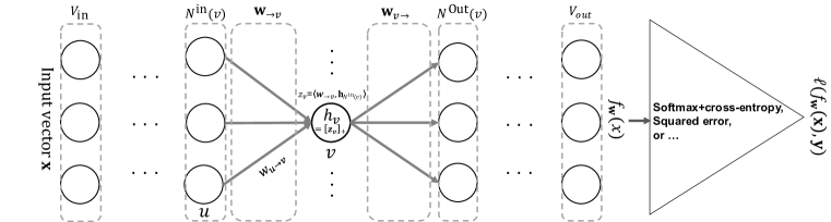
We denote $N^{\text{in}}(v)=\left\{u\middle|(u\rightarrow v)\in E\right\}$ and $N^{\text{out}}(v)=\left\{u\middle|(v\rightarrow u)\in E\right\}$, the sets of nodes feeding into $v$ and that $v$ feeds into. We can then write $\mathbf{h}_{N^{\text{in}}(v)}\in\mathbb{R}^{\left|N^{\text{in}}(v)\right|}$ for the vector of outputs feeding into $v$, and $\mathbf{w}_{\rightarrow v}\in\mathbb{R}^{\left|N^{\text{in}}(v)\right|}$ for the vector of weights of unit $v$, so that $z_{v}=\left\langle\mathbf{w}_{\rightarrow v},\mathbf{h}_{N^{\text{in}}(v)}\right\rangle$.

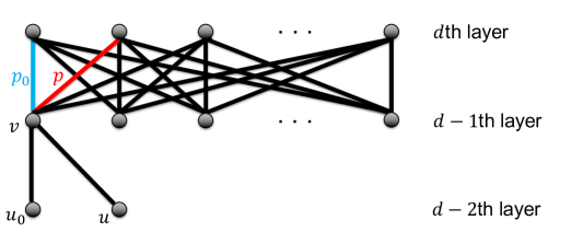
We do not restrict to layered networks, nor do we ever need to explicitly discuss layers, and can instead focus on a single node at a time (we view this as the main advantage of the graph notation). But to help those more comfortable with layered networks understand the notation, let us consider a layered fully-connected network: The nodes are partitioned into layers $V=V_{0}\cup V_{1}\cup\ldots V_{d}$, with $V_{\rm in}=V_{0}$, $V_{\rm out}=V_{d}$. For all nodes $v\in V_{i}$ on layer $i$, $N^{\text{in}}(v)$ is the same and equal to $N^{\text{in}}(v)=V_{i-1}$, and so $\mathbf{h}_{N^{\text{in}}(v)}=\mathbf{h}_{V_{i-1}}$ consists of all outputs from the previous layer and we recover the layered recursive formula $h_{v}=[\left\langle\mathbf{w}_{\rightarrow v},\mathbf{h}_{V_{i-1}}\right\rangle]_{+}$ and $\mathbf{h}_{V_{i}}=[\mathbf{W}_{i}\mathbf{h}_{V_{i-1}}]_{+}$, where $\mathbf{W}\in\mathbb{R}^{\left|V_{i}\right|\times\left|V_{i-1}\right|}$ is a matrix with entries $w_{u\rightarrow v}$, for each $u\in V_{i-1},v\in V_{i}$. This description ignores the bias term, which could be modeled as a direct connection from $v_{\rm bias}$ into every node on every layer, or by introducing a bias unit (with output fixed to 1) at each layer. Please see Figure 1 for an example of a layered feedforward network and a summary of notation used in the paper.

Symbol	Meaning	Symbol	Meaning
$\mathbf{x}$ / $\mathbf{y}$	input vector / label	$V_{\text{in}}$ / $V_{\text{out}}$	the set of input / output nodes
$\mathbf{w}$	the parameter vector	$w_{u\rightarrow v}$	the weight of the edge $(u\rightarrow v)$
$\mathbf{w}_{v\rightarrow}$	the vector of incoming weights to $v$	$\mathbf{w}_{\rightarrow v}$	the vector of outgoing weights from $v$
$N^{\text{in}}(v)$	the set of nodes feeding into $v$	$N^{\text{out}}(v)$	the set of nodes that $v$ feeds into
$h_{v}$	the output value of node $v$	$z_{v}$	the activation value of node $v$

Figure 1: An example of layered feedforward networks and notation used in the paper

We consider supervised training tasks, where each input $\mathbf{x}$ is associated with a desired label $y$ and how well the network captures this label is quantified by a loss function $\ell(f_{\mathbf{w}}(\mathbf{x}),y)$. For example, in a classification problem $y$ is one of $|V_{\rm out}|$ classes and a cross-entropy (soft-max) loss might be used. We also refer to a source distribution $\mathcal{D}_{(\mathbf{x},\mathbf{y})}$ over input-label pairs, where the goal is to minimize the expected loss:

$$L_{\mathcal{D}}(\mathbf{w})=\mathbb{E}_{(\mathbf{x},y)\sim\mathcal{D}}\left[\ell(f_{\mathbf{w}}(\mathbf{x}),y)\right]$$ (1)

All expectations, unless specified otherwise, refer to expectation w.r.t. this source distribution.

Invariances and Node-wise Rescaling

Once the architecture (graph $G$) is fixed, every choice of weight $\mathbf{w}$ defines a function $f_{\mathbf{w}}$. But this parameterization is not unique–the same function $f$ could be parameterized by two different weight settings (i.e. we could have $f_{\mathbf{w}}=f_{\mathbf{w}^{\prime}}$ even though $\mathbf{w}\not=\mathbf{w}^{\prime}$). Ideally, we’d like to work as directly as possibly on the functions rather then the parameterization. It is therefor important to understand different “invariances”, i.e. different transformations that can be applied to the weights without changing the function. We note that the notion of invariance we define here is tied to a fixed network architecture $G$: we do not consider transformation that changes the network architecture, such as insertion of a linear layer (as in, e.g. Ollivier, 2015).

We say that network $G$ is invariant to an invariant transformation $T(\mathbf{w})$, iff for any weight setting $\mathbf{w}$, $f_{\mathbf{w}}=f_{T(\mathbf{w})}$. We say that an update rule $\mathcal{A}$ (e.g. a rule for obtaining the next iterate from the current iterate in an optimization procedure) is invariant to transformation $T$ iff for any weight setting $\mathbf{w}$, $f_{\mathcal{A}(\mathbf{w})}=f_{\mathcal{A}(T(\mathbf{w}))}$. That is, whether we start an iterative optimization procedure using updates $\mathcal{A}$ at $\mathbf{w}$ or the at the equivalent $\mathbf{w}^{\prime}=T(\mathbf{w})$, we would always be working on the same function (only with a different parameterization).

An important invariance in feedforward ReLU network is node-wise rescaling (or rebalancing). For any positive scalar $\rho$ and for any internal node $v$ ($v\notin V_{\rm in}$ and $v\notin V_{\rm out}$), we can scale all the incoming weights into $v$ by $\rho$ and all the outgoing weights by $1/\rho$ without changing the computation in the networks. That is, the following transformation $\mathbf{w}^{\prime}=T(\mathbf{w})$ satisfies $f_{\mathbf{w}}=f_{\mathbf{w}^{\prime}}$:

$$w^{\prime}_{v\rightarrow u} =\rho w_{v\rightarrow u}\quad(\forall u\in N^{\text{out}}(u)),$$ (2)

$$w^{\prime}_{u\rightarrow v} =\rho^{-1}w_{u\rightarrow v}\quad(\forall u\in N^{\text{in}}(v))$$

$$w^{\prime}_{u\rightarrow u^{\prime}} =w_{u\rightarrow u^{\prime}}\quad(\textrm{otherwise})$$

We can combined multiple such rescalings to push the scaling up or down the network without changing the computation. One of our goals is obtaining optimization algorithms that are invariant to such transformations.

$R_{v}$	20cmMeasure	Normalized reparametrization	Diagonal steepest descent
$D=\operatorname{diag}\left(\bm{\gamma}^{2}_{N^{\text{in}(v)}}\right)$	Path-Norm	Unit-wise Path-Normalization	Path-SGD
$C=\text{Cov}\left(\mathbf{h}_{N^{\text{in}(v)})}\right)$	Variance	Batch-Normalization
$M=\mathbb{E}\left[\mathbf{h}_{N^{\text{in}(v)})}\mathbf{h}_{N^{\text{in}(v)})}^{\top}\right]$	Second Moment		Diag. Natural Gradient
20cm$\alpha M+(1-\alpha)D$
$\alpha C+(1-\alpha)D$	DDP-Norm	DDP-Normalization	DDP-SGD
Node-wise Rescaling Invariant	Yes	No	Yes

Table 1: Some of the choices for $R_{v}$ in the proposed unified framework.

3 A Unified Framework

We define a complexity measure on each node as follows:

$$\gamma_{v}(\mathbf{w})=\sqrt{\mathbf{w}_{\rightarrow v}^{\top}R_{v}\mathbf{w}_{\rightarrow v}}$$ (3)

where $R_{v}$ is a positive semidefinite matrix that could depend on the computations feeding into $v$, and captures both the complexity of the nodes feeding into $v$ and possibly their interactions. We consider several possibilities for $R_{v}$, summarized also in Table 1.

A first possibility is to set $R_{v}=\operatorname{diag}\left(\bm{\gamma}^{2}_{N^{\text{in}(v)}}\right)$ to a diagonal matrix consisting of the complexities of the incoming units. This choice does not depend on the source distribution (i.e. the data), and also ignores the effect of activations (since the activation pattern depends on the input distribution) and of dependencies between different paths in the network. Intuitively, with this choice of $R_{v}$, the measure $\gamma_{v}(\mathbf{w})$ captures the “potential” (data independent) variability or instability at the node.

Another possibility is to set $R_{v}$ to either the covariance (centralized second moment) or to the (uncentralized) second moment matrix of the outputs feeding into $v$. In this case, $\gamma^{2}_{v}(\mathbf{w})$ would evaluate to the variance or (uncentralized) second moment of $z_{v}$. We could also linearly combined the data independent measure, which measures inherent instability, with one of these the data-dependent measure to obtain:

$$\gamma^{2}_{v}(\mathbf{w})=\alpha S(z_{v})+(1-\alpha)\sum_{u\in N^{\text{in}}(v)}\gamma^{2}_{u}(\mathbf{w})w^{2}_{u\rightarrow v}\quad(v\notin V_{\rm in}),$$ (4)

where $S(z_{v})$ is either the variance or uncentralized second moment, and $\alpha$ is a parameter.

The complexity measure above is defined for each node of the network separately, and propagates through the network. To get an overall measure of complexity we sum over the output units and define the following complexity measure for the function $f_{\mathbf{w}}$ as represented by the network:

$$\gamma^{2}_{\rm net}(\mathbf{w})=\sum_{v\in V_{\rm out}}\gamma^{2}_{v}(\mathbf{w}).$$ (5)

For $R_{v}=\operatorname{diag}\left(\bm{\gamma}^{2}_{N^{\text{in}(v)}}\right)$, this complexity measure agrees with the $\ell_{2}$-Path-regularizer as introduced by Neyshabur et al. (2015b). This is the sum over all paths in the network of the squared product of weights along the path. The path-regularizer is also equivalent to looking at the minimum over all “node rescalings” of $\mathbf{w}$ (i.e. all possibly rebalancing of weights yielding the same function $f_{\mathbf{w}}$) of the $\max_{v}\left\lVert{\mathbf{w}_{\rightarrow v}}\right\rVert$. But, unlike this max-norm measure, the path-regularizer does not depend on the rebalancing and is invariant to node rescalings (Neyshabur et al., 2015b).

For data-dependent choices of $R_{v}$, we also get a similar invariance property. We refer to the resulting complexity measure, $\gamma^{2}_{\rm net}(\mathbf{w})$, as the Data-Dependent-Path (DDP) regularizer.

After choosing $R_{v}$, we will think of $\gamma_{v}$ as specifying the basic “geometry” and bias (for both optimization and learning) over weights. In terms of learning, we will (implicitly) prefer weights with smaller $\gamma_{v}$ measure, and correspondingly in terms of optimization we will bias toward smaller $\gamma_{v}$ “balls” (i.e. search over the part of the space where $\gamma_{v}$ is smaller). We will consider two basic ways of doing this: In Section 4 we will consider methods that explicitly try to keep $\gamma_{v}$ small for all internal nodes in the network, that is explicitly search over simpler weights. Any scaling is pushed to the output units, and this scaling hopefully does not grow too much due. In Section 5 we will consider (approximate) steepest descent methods with respect to the overall $\gamma_{\rm net}$, i.e. updates that aim at improving the training objective while being small in terms of their effect on $\gamma_{\rm net}$.

4 DDP-Normalization: A Batch-Normalization Approach

In this Section, we discuss an optimization approach based on ensuring $\gamma_{v}$ for all internal nodes $v$ are fixed and equal to one—that is, the complexity of all internal nodes is “normalized”, and any scaling happens only at the output nodes. We show that with a choice of $R_{v}=\text{Cov}\left(\mathbf{h}_{N^{\text{in}(v)})}\right)$, this is essentially equivalent to Batch Normalization (Ioffe & Szegedy, 2015).

Batch-Normalization Ioffe & Szegedy (2015) was suggested as an alternate architecture, with special “normalization” layers, that ensure the variance of node outputs are normalized throughout training. Considering a feed-forward network as a graph, for each node $v$, the Batch-Normalization architecture has as parameters an (un-normalized) incoming weight vector $\tilde{\mathbf{w}}$ and two additional scalars $c_{v},b_{v}\in\mathbb{R}$ specifying scaling and shift respectively. The function computed by the network is then given by a forward propagation similar to standard feed-forward ReLU networks as described in Section 2, except that for each node an un-normalized activation is first computed:

$$\tilde{z}_{v}=\left\langle\tilde{\mathbf{w}}_{\rightarrow v},\mathbf{h}_{N^{\text{in}}(v)}\right\rangle$$ (6)

Then, this activation is normalized to obtain the normalized activation, which is also scaled and shifted, and the output of the unit is the output of the activation function for this activation value:

$$\begin{gathered}z_{v}=c_{v}\frac{\tilde{z}_{v}-\mathbb{E}[\tilde{z_{v}}]}{\sqrt{\text{Var}(\tilde{z}_{v})}}+b_{v}\\ h_{v}=[z_{v}]_{+}\end{gathered}$$ (7)

The variance and expectation are actually calculated on a “mini-batch” of training examples, giving the method its name. Batch-normalization then proceeds by training the architecture specified in (6) and (7) through mini-batch stochastic gradient descent, with each gradient mini-batch also used for estimating the variance and expectation in (7) for all points in the mini-batch.

Instead of viewing batch-normalization as modifying the architecture, or forward propagation, we can view it as a re-parameterization, or change of variables, of the weights in standard feed-forward networks as specified in Section 2. In particular, instead of specifying the weights directly through $\mathbf{w}$, we specify them through $\tilde{\mathbf{w}},\mathbf{b}$ and $\mathbf{c}$, with the mapping:

$$\tilde{\gamma}^{2}_{v}=\tilde{\mathbf{w}}_{\rightarrow v}^{\top}R_{v}\tilde{\mathbf{w}}_{\rightarrow v}\quad\quad R_{v}=\text{Cov}(h_{N^{\text{in}}(v)})$$ (8)

$$w_{u\rightarrow v}=\begin{cases}c\frac{\tilde{w}_{u\rightarrow v}}{\tilde{\gamma}_{v}}&u\neq v_{\text{bias}}\\ b-c\frac{\mathbb{E}\left[\left\langle\tilde{\mathbf{w}}_{\rightarrow v},\mathbf{h}_{N^{\text{in}}(v)}\right\rangle\right]}{\tilde{\gamma}_{v}}&u=v_{\text{bias}}\\ \end{cases}$$ (9)

The model class of functions used by Batch-Normalization is thus exactly the same model class corresponding to standard feed-forward network, just the parameterization is different. However, the change of variables from $\mathbf{w}$ to $\tilde{\mathbf{w}},\mathbf{b},\mathbf{c}$ changes the geometry implied by the parameter space, and consequently the trajectory (in model space) of gradient updates—effectively transforming the gradient direction by the Jacobian between the two parameterizations. Batch-Normalization can thus be viewed as an alternate optimization on the same model class as standard feed-forward networks, but with a different geometry. The reparametrization ensures that $\gamma_{v}(\mathbf{w})=c_{v}$ for all nodes—that is, the complexity is explicit in the parameterization and thus gets implicitly regularized through the implicit regularization inherent in stochastic gradient updates.

The re-parameterization (9) is redundant and includes more parameters than the original parameterization $\mathbf{w}$—in addition to one parameter per edge, it includes also two additional parameters per node, namely the shift $b_{v}$ and scaling $c_{v}$. The scaling parameters at internal nodes can be avoided and removed by noting that in ReLU networks, due to the node-rescaling property, all scaling can be done at the output nodes. That is, fixing $c_{v}=1$ for all internal $v$ does not actually change the model class (all functions realizable by the model can be realized this way). Similarly, we can also avoid the additional shift parameter $b_{v}$ and rely only on bias units and bias weights $\tilde{w}_{v_{\rm bias}\rightarrow v}$ that get renormalized together with weights. The bias term $\tilde{w}_{v_{\rm bias}\rightarrow v}$ does not affect normalization (since it is deterministic and so has no effect on the variance), it just gets rescaled with the other weights.

We thus propose using a simpler reparametrization (change of variables), with the same number of parameters, using only $\tilde{\mathbf{w}}$ and defining for each internal unit:

$$w_{u\rightarrow v}=\frac{\tilde{w}_{u\rightarrow v}}{\tilde{\gamma}_{v}}$$ (10)

with $\tilde{\gamma}_{v}$ as in (8), and with the output nodes un-normalized: $\mathbf{w}_{\rightarrow V_{\rm out}}=\tilde{\mathbf{w}}_{\rightarrow V_{\rm out}}$. This ensures that for all internal nodes $\gamma_{v}(\mathbf{w})=1$.

Going beyond Batch-Normalization, we can also use the same approach with other choices of $R_{v}$, including all those in Table 1: We work with a reparametrization $\tilde{\mathbf{w}}$, defined through (8) and (10) but with different choices of $R_{v}$, and take gradient (or stochastic gradient) steps with respect to $\tilde{\mathbf{w}}$. Expectations in the definition of $R_{v}$ can be estimated on the stochastic gradient descent mini-batch as in Batch-Normalization, or on independent samples of labeled or unlabeled examples. We refer to such methods as “DDP-Normalized” optimization. Gradients in DDP-Normalization can be calculated implemented very efficiently similar to Batch-Normalization (see Appendix A.1).

When using this type of DDP-Normalization, we ensure that for any internal node $\gamma_{v}(\mathbf{w})=1$ (the value of $\tilde{\gamma}_{v}$ can be very different from $1$, but what is fixed is the value of $\gamma_{v}$ as defined in (3) in terms of the weights $\mathbf{w}$, which in turn can be derived from $\tilde{\mathbf{w}}$ through (9)), and so the overall complexity $\gamma_{\rm net}(\mathbf{w})$ depends only on the scaling at the output layer.

Another interesting property of DDP-Normalization updates is that for any internal node $v$, the updates direction of $\tilde{w}_{\rightarrow v}$ is exactly orthogonal to the weights:

Theorem 1.

For any weight $\tilde{\mathbf{w}}$ in DDP-Normalization and any non-input node $v\notin V_{\text{in}}$

$$\left\langle\tilde{\mathbf{w}}_{\rightarrow v},\frac{\partial L}{\partial\tilde{\mathbf{w}}_{\rightarrow v}}\right\rangle=0$$ (11)

The fact that the gradient is orthogonal to the parameters means weight updates in DDP-Normalization are done in a way that it prevents the norm of weights to change considerably after each updates (the proof is given in Appendix C).

5 DDP-SGD

We now turn to a more direct approach of using our complexity measure for optimization. To do so, let us first recall the strong connection between geometry, regularization and optimization through the specific example of gradient descent.

Gradient descent can be thought of as steepest descent with respect to the Euclidean norm—that is, it takes a step in a direction that maximizes improvement in the objective while also being small in terms of the Euclidean norm of the step. The step can also be viewed as a regularized optimization of the linear approximation given by the gradient, where the regularizer is squared Euclidean norm. Gradient Descent is then inherently linked to the Euclidean norm—runtime of optimization is controlled by the Euclidean norm of the optimum and stochastic gradient descent yields implicit Euclidean norm regularization. A change in norm or regularizer, which we think of as a change of geometry, would then yield different optimization procedure linked to that norm.

What we would like is to use the DDP-regularizer $\gamma_{\rm{\rm net}}(\mathbf{w})$ to define our geometry, and for that we need a distance (or divergence) measure corresponding to it by which we can measure the “size” of each step, and require steps to be small under this measure. We cannot quite do this, but instead we use a diagonal quadratic approximation of $\gamma_{\rm net}(\mathbf{w})$ about our current iterate, and then take a steepest descent step w.r.t. the quadratic norm defined by this approximation.

Specifically, given a choice of $R_{v}$ and so complexity measure $\gamma_{\rm net}(\mathbf{w})$, for the current iterate $\mathbf{w}^{(t)}$ we define the following quadratic approximation:

$$\hat{\gamma}^{2}_{\rm net}(\mathbf{w}^{(t)}+\Delta\mathbf{w})=\gamma^{2}_{\rm net}(\mathbf{w}^{(t)})+\left\langle\nabla\gamma^{2}_{\rm net}(\mathbf{w}^{(t)}),\Delta\mathbf{w}\right\rangle+\frac{1}{2}\Delta\mathbf{w}^{\top}\operatorname{diag}\left(\nabla^{2}\gamma^{2}_{\rm net}(\mathbf{w}^{(t)})\right)\Delta\mathbf{w}$$ (12)

and the corresponding quadratic norm:

$$\left\lVert{\mathbf{w}^{\prime}-\mathbf{w}}\right\rVert^{2}_{\hat{\gamma}^{2}_{\rm net}}=\left\lVert{\mathbf{w}^{\prime}-\mathbf{w}}\right\rVert^{2}_{\operatorname{diag}(\frac{1}{2}\nabla^{2}\gamma^{2}_{\rm net}(\mathbf{w}^{(t)}))}=\sum_{(u\rightarrow v)\in G}\frac{1}{2}\frac{\partial^{2}\gamma^{2}_{\rm net}}{\partial\mathbf{w}^{2}_{u\rightarrow v}}(\mathbf{w}^{\prime}_{u\rightarrow v}-\mathbf{w}_{u\rightarrow v})^{2}.$$ (13)

We can now define the DDP-update as:

$$\mathbf{w}^{(t+1)}=\min_{\mathbf{w}}\eta\left\langle\nabla L(w),\mathbf{w}-\mathbf{w}^{(t)}\right\rangle+\frac{1}{2}\left\lVert{\mathbf{w}^{\prime}-\mathbf{w}}\right\rVert^{2}_{\hat{\gamma}^{2}_{\rm net}}.$$ (14)

Another way of viewing the above approximation is as taking a diagonal quadratic approximation of the Bergman divergence of the regularizer. Solving (14) yields the update:

$$w^{(t+1)}_{u\rightarrow v}=w_{u\rightarrow v}-\frac{\eta}{\kappa_{u\rightarrow v}(\mathbf{w})}\frac{\partial L}{\partial w_{u\rightarrow v}}(\mathbf{w}^{(t)})\quad\quad\textrm{where: }\kappa_{u\rightarrow v}(\mathbf{w})=\frac{1}{2}\frac{\partial^{2}\gamma^{2}_{\rm net}}{\partial w^{2}_{u\rightarrow v}}.$$ (15)

Instead of using the full gradient, we can also use a limited number of training examples to obtain stochastic estimates of $\frac{\partial L}{\partial w_{u\rightarrow v}}(\mathbf{w}^{(t)})$—we refer to the resulting updates as DDP-SGD.

For the choice $R_{v}=\operatorname{diag}(\gamma^{2}_{N^{\text{in}}(v)})$, we have that $\gamma^{2}_{\rm net}$ is the Path-norm and we recover Path-SGD Neyshabur et al. (2015a). As was shown there, the Path-SGD updates can be calculated efficiently using a forward and backward propagation on the network, similar to classical back-prop. In Appendix A.2 we show how this type of computation can be done more generally also for other choices of $R_{v}$ in Table 1.

Relation to the Natural Gradient

The DDP updates are similar in some ways to Natural Gradient updates, and it is interesting to understand this connection. Like the DDP, the Natural Gradients direction is a steepest descent direction, but it is based on a divergence measure calculated directly on the function $f_{\mathbf{w}}$, and not the parameterization $\mathbf{w}$, and as such is invariant to reparametrizations. The natural gradient is defined as a steepest descent direction with respect to the KL-divergence between probability distributions, and so to refer to it we must refer to some probabilistic model. In our case, this will be a conditional probability model for labels $\mathbf{y}$ conditioned on the inputs $\mathbf{x}$, taking expectation with respect to the true marginal data distribution over $\mathbf{x}$.

What we will show that for the choice $R_{v}=\mathbb{E}[\mathbf{h}_{N^{\text{in}}(v)}\mathbf{h}_{N^{\text{in}}(v)}^{\top}]$, the DDP update can also be viewed as an approximate Natural Gradient update. More specifically, it is a diagonal approximation of the Natural Gradient for a conditional probability model $q(\mathbf{y}|\mathbf{x};\mathbf{w})$ (of the labels $\mathbf{y}$ given an input $\mathbf{x}$) parametrized by $\mathbf{w}$ and specified by adding spherical Gaussian noise to the outputs of the network: $\mathbf{y}|\mathbf{x}\sim\mathcal{N}(f_{\mathbf{w}}(\mathbf{x}),I_{|V_{\rm out}|})$.

Given the conditional probability distribution $q(\mathbf{y}|{\mathbf{x}};\mathbf{w})$, we can calculate the expected Fisher information matrix. This is a matrix indexed by parameters of the model, in our case edges $e=(u\rightarrow v)$ on the graph and their corresponding weights $w_{e}$, with entries defined as follows:

$$F({\mathbf{w}})[e,e^{\prime}]=\mathbb{E}_{{\mathbf{x}}\sim p(\mathbf{x})}\mathbb{E}_{\mathbf{y}\sim q(\mathbf{y}|{\mathbf{x}};\mathbf{w})}\left[\frac{\partial\log q(\mathbf{y}|{\mathbf{x}};\mathbf{w})}{\partial w_{e}}\frac{\partial\log q(\mathbf{y}|{\mathbf{x}};\mathbf{w})}{\partial w_{e^{\prime}}}\right],$$ (16)

where $x\sim p(\mathbf{x})$ refers to the marginal source distribution (the data distribution). That is, we use the true marginal distributing over $\mathbf{x}$, and the model conditional distribution $\mathbf{y}|\mathbf{x}$, ignoring the true labels. The Natural Gradient updates can then be written as(see appendix B for more information):

$$\mathbf{w}^{(t+1)}=\mathbf{w}^{(t)}-\eta F(\mathbf{w}^{(t)})^{-1}\nabla_{\mathbf{w}}L(\mathbf{w}^{(t)}).$$ (17)

If we approximate the Fisher information matrix with its diagonal elements, the update step normalizes each dimension of the gradient with the corresponding element on the diagonal of the Fisher information matrix:

$$w^{(t+1)}_{e}=w^{(t)}_{e}-\frac{\eta}{F(\mathbf{w})[e,e]}\frac{\partial L}{\partial w_{e}}(\mathbf{w}^{(t)}).$$ (18)

Using diagonal approximation of Fisher information matrix to normalize the gradient values has been suggested before as a computationally tractable alternative to the full Natural Gradient (LeCun et al., 1998; Schaul et al., 2013). Ollivier (2015) also suggested a “quasi-diagonal” approximations that includes, in addition to the diagonal, also some non-diagonal terms corresponding to the relationship between the bias term and every other incoming weight into a unit.

For our Gaussian probability model, where $\log q(\mathbf{y}|\mathbf{x})=\frac{1}{2}\left\lVert{\mathbf{y}-f_{\mathbf{w}}(\mathbf{x})}\right\rVert^{2}+{\rm const}$, the diagonal can be calculated as:

$$F(\mathbf{w})[e,e]=\mathbb{E}_{\mathbf{x}\sim p(\mathbf{x})}\left[\sum_{v^{\prime}\in V_{\text{out}}}\left(\frac{\partial f_{\mathbf{w}}(\mathbf{x})[v^{\prime}]}{\partial w_{e}}\right)^{2}\right],$$ (19)

using (62). We next prove that this update is equivalent to DDP-SGD for a specific choice of $R_{v}$, namely the second moment.

Theorem 2.

The Diagonal Natural Gradient indicated in equations (18) and  (19) is equivalent to DDP-SGD for $R_{v}=\mathbb{E}\left[\mathbf{h}_{N^{\text{in}}(v)}\mathbf{h}_{N^{\text{in}}(v)}^{\top}\right]$.

Proof.

We calculate the scaling factor $\kappa_{u\rightarrow v}(\mathbf{w})$ for DDP-SGD as follows:

$$\kappa_{u\rightarrow v}(\mathbf{w}) =\frac{1}{2}\frac{\partial^{2}\gamma^{2}_{\rm net}}{\partial w_{u\rightarrow v}^{2}}=\frac{1}{2}\sum_{v^{\prime}\in V_{\text{out}}}\frac{\partial^{2}\mathbb{E}[z^{2}_{v^{\prime}}]}{\partial w_{u\rightarrow v}^{2}}=\sum_{v^{\prime}\in V_{\text{out}}}\frac{\partial}{\partial w_{u\rightarrow v}}\left(\frac{1}{2}\frac{\partial\mathbb{E}[z^{2}_{v^{\prime}}]}{\partial w_{u\rightarrow v}}\right)$$

$$=\sum_{v^{\prime}\in V_{\text{out}}}\frac{\partial}{\partial w_{u\rightarrow v}}\left(\mathbb{E}\left[z_{v^{\prime}}\frac{\partial z_{v^{\prime}}}{\partial w_{u\rightarrow v}}\right]\right)=\sum_{v^{\prime}\in V_{\text{out}}}\frac{\partial}{\partial w_{u\rightarrow v}}\left(\mathbb{E}\left[z_{v^{\prime}}h_{u}\frac{\partial z_{v^{\prime}}}{\partial z_{v}}\right]\right)$$

$$=\sum_{v^{\prime}\in V_{\text{out}}}\mathbb{E}\left[h^{2}_{u}\left(\frac{\partial z_{v^{\prime}}}{\partial z_{v}}\right)^{2}\right]=\mathbb{E}\left[h^{2}_{u}\sum_{v^{\prime}\in V_{\text{out}}}\left(\frac{\partial z_{v^{\prime}}}{\partial z_{v}}\right)^{2}\right]$$

$$=\mathbb{E}\left[\sum_{v^{\prime}\in V_{\text{out}}}\left(\frac{\partial f_{\mathbf{w}}(\mathbf{x})[v^{\prime}]}{\partial w_{e}}\right)^{2}\right]=F(\mathbf{w})[u\rightarrow v,u\rightarrow v]$$

Therefore, the scaling factors in DDP-SGD with $R_{v}=\mathbb{E}\left[\mathbf{h}_{N^{\text{in}}(v)}\mathbf{h}_{N^{\text{in}}(v)}^{\top}\right]$ are exactly the diagonal elements of the Fisher Information matrix used in the Natural Gradient updates. ∎

6 Node-wise invariance

In this section, we show that DDP-SGD is invariant to node-wise rescalings (see Section 2), while DDP-Normalization does not have favorable invariance properties.

6.1 DDP-SGD on feedforward networks

In Section 2, we observed that feedforward ReLU networks are invariant to node-wise rescaling. To see if DDP-SGD is also invariant to such rescaling, consider a rescaled $\mathbf{w}^{\prime}=T(\mathbf{w})$, where $T$ is a rescaling by $\rho$ at node $v$ as in (2). Let $\mathbf{w}^{+}$ denote the weights after a step of DDP-SGD. To establish invariance to node-rescaling we need to show that $\mathbf{w}^{\prime+}=T(\mathbf{w}^{+})$. For the outgoing weights from $v$ we have:

$$w^{\prime+}_{v\rightarrow j} =\rho w_{v\rightarrow j}-\frac{\rho^{2}\eta}{\kappa_{v\rightarrow j}(\mathbf{w})}\frac{\partial L}{\rho\partial w_{v\rightarrow j}}(\mathbf{w})$$

$$=\rho\left(w_{v\rightarrow j}-\frac{\eta}{\kappa_{v\rightarrow j}(\mathbf{w})}\frac{\partial L}{\partial w_{v\rightarrow j}}(\mathbf{w})\right)=\rho w^{+}_{v\rightarrow j}$$

Similar calculations can be done for incoming weights to the node $v$. The only difference is that $\rho$ will be substituted by $1/\rho$. Moreover, note that due to non-negative homogeneity of ReLU activation function, the updates for the rest of the weights remain exactly the same. Therefore, DDP-SGD is node-wise rescaling invariant.

6.2 SGD on DDP-Normalized networks

Since DDP-Normalized networks are reparametrization of feedforward networks, their invariances are different. Since the operations in DDP-Normalized networks are based on $\tilde{w}$, we should study the invariances for $\tilde{w}$. The invariances in this case are given by rescaling of incoming weights into a node, i.e. for an internal node $v$ and scaling $\rho>0$:

$$T(\tilde{w})_{k\rightarrow v}=\rho\tilde{w}_{k\rightarrow v}\quad(\forall k\in N^{\text{in}}(v))$$

while all other weights are unchanged. The DDP-Normalized networks are invariant to the above transformation because the output of each node is normalized. The SGD update rule is however not invariant to this transformation:

$$T(\tilde{w})^{+}_{k\rightarrow v} =\rho\tilde{w}_{k\rightarrow v}-\eta\frac{\partial L}{\rho\partial\tilde{w}_{k\rightarrow v}}(\tilde{\mathbf{w}})\neq\rho\left(\tilde{w}_{k\rightarrow v}-\eta\frac{\partial L}{\partial\tilde{w}_{k\rightarrow v}}(\tilde{\mathbf{w}})\right)=\rho\tilde{w}^{+}_{k\rightarrow v}$$

7 Understanding Invariances

The goal of this section is to discuss whether being invariant to node-wise rescaling transformations is sufficient or not.

Ideally we would like our algorithm to be at least invariant to all the transformations to which the model $G$ is invariant. Note that this is different than the invariances studied in Ollivier (2015), in that they study algorithms that are invariant to reparametrizations of the same model but we look at transformations within the the parameter space that preserve the function in the model. This will eliminate the need for non-trivial initialization. Thus our goal is to characterize the whole variety of transformations to which the model is invariant and check if the algorithm is invariant to all of them.

We first need to note that invariance can be composed. If a network $G$ is invariant to transformations $T_{1}$ and $T_{2}$, it is also invariant to their composition $T_{1}\circ T_{2}$. This is also true for an algorithm. If an algorithm is invariant to transformations $T_{1}$ and $T_{2}$, it is also invariant to their composition. This is because $f_{T_{2}\circ T_{1}\circ\mathcal{A}({\mathbf{w}})}=f_{T_{2}\circ\mathcal{A}(T_{1}\circ{\mathbf{w}})}=f_{\mathcal{A}(T_{2}\circ T_{1}({\mathbf{w}}))}$.

Then it is natural to talk about the basis of invariances. The intuition is that although there are infinitely many transformations to which the model (or an algorithm) is invariant, they could be generated as compositions of finite number of transformations.

In fact, in the infinitesimal limit the directions of infinitesimal changes in the parameters to which the function $f_{{\mathbf{w}}}$ is insensitive form a subspace. This is because for a fixed input ${\mathbf{x}}$, we have

$$f_{{\mathbf{w}}+\bm{\Delta}}(x)=f_{{\mathbf{w}}}({\mathbf{x}})+\sum\nolimits_{e\in E}\frac{\partial f_{{\mathbf{w}}}({\mathbf{x}})}{\partial w_{e}}\cdot\Delta_{e}+O(\|\bm{\Delta}\|^{2}),$$ (20)

where $E$ is the set of edges, due to a Taylor expansion around ${\mathbf{w}}$. Thus the function $f_{{\mathbf{w}}}$ is insensitive (up to $O(\|\bm{\Delta}\|^{2})$) to any change in the direction $\bm{\Delta}$ that lies in the (right) null space of the Jacobian matrix $\partial f_{{\mathbf{w}}}({\mathbf{x}})/\partial{\mathbf{w}}$ for all input ${\mathbf{x}}$ simultaneously. More formally, the subspace can be defined as

$$N({\mathbf{w}})=\bigcap\nolimits_{{\mathbf{x}}\in\mathbb{R}^{|V_{\rm in}|}}\textrm{Null}\left(\frac{\partial f_{{\mathbf{w}}}({\mathbf{x}})}{\partial{\mathbf{w}}}\right).$$ (21)

Again, any change to ${\mathbf{w}}$ in the direction $\bm{\Delta}$ that lies in $N({\mathbf{w}})$ leaves the function $f_{{\mathbf{w}}}$ unchanged (up to $O(\|\bm{\Delta}\|^{2})$) at every input $x$. Therefore, if we can calculate the dimension of $N({\mathbf{w}})$ and if we have ${\rm dim}N({\mathbf{w}})=|V_{\rm internal}|$, where we denote the number of internal nodes by $|V_{\rm internal}|$, then we can conclude that all infinitesimal transformations to which the model is invariant can be spanned by infinitesimal node-wise rescaling transformations.

Note that the null space $N({\mathbf{w}})$ and its dimension is a function of ${\mathbf{w}}$. Therefore, there are some points in the parameter space that have more invariances than other points. For example, suppose that $v$ is an internal node with ReLU activation that receives connections only from other ReLU units (or any unit whose output is nonnegative). If all the incoming weights to $v$ are negative including the bias, the output of node $v$ will be zero regardless of the input, and the function $f_{{\mathbf{w}}}$ will be insensitive to any transformation to the outgoing weights of $v$. Nevertheless we conjecture that as the network size grows, the chance of being in such a degenerate configuration during training will diminish exponentially.

When we study the dimension of $N({\mathbf{w}})$, it is convenient to analyze the dimension of the span of the row vectors of the Jacobian matrix $\partial f_{{\mathbf{w}}}({\mathbf{x}})/\partial{\mathbf{w}}$ instead. We define the degrees of freedom of model $G$ at ${\mathbf{w}}$ as

$$d_{G}({\mathbf{w}})={\rm dim}\left(\bigcup\nolimits_{{\mathbf{x}}\in\mathbb{R}^{|V_{\rm in}|}}{\rm Span}\left(\frac{\partial f_{{\mathbf{w}}}({\mathbf{x}})}{\partial{\mathbf{w}}}[v,:]:v\in V_{\rm out}\right)\right),$$ (22)

where $\partial f_{{\mathbf{w}}}({\mathbf{x}})[v,:]/\partial{\mathbf{w}}$ denotes the $v$th row vector of the Jacobian matrix and ${\mathbf{x}}$ runs over all possible input ${\mathbf{x}}$. Intuitively, $d_{G}({\mathbf{w}})$ is the dimension of the set of directions that changes $f_{{\mathbf{w}}}(x)$ for at least one input $x$.

Due to the rank nullity theorem $d_{G}({\mathbf{w}})$ and the dimension of $N({\mathbf{w}})$ are related as follows:

$$d_{G}({\mathbf{w}})+{\rm dim}\left(N({\mathbf{w}})\right)=|E|,$$

where $|E|$ is the number of parameters. Therefore, again if $d_{G}({\mathbf{w}})=|E|-|V_{\rm internal}|$, then we can conclude that infinitesimally speaking, all transformations to which the model is invariant can be spanned by node-wise rescaling transformations.

Considering only invariances that hold uniformly over all input ${\mathbf{x}}$ could give an under-estimate of the class of invariances, i.e., there might be some invariances that hold for many input ${\mathbf{x}}$ but not all. An alternative approach for characterizing invariances is to define a measure of distance between functions that the neural network model represents based on the input distribution, and infinitesimally study the subspace of directions to which the distance is insensitive. We can define distance between two functions $f$ and $g$ as

$$D(f,g)=\mathbb{E}_{{\mathbf{x}}\sim\mathcal{D}}\left[m(f({\mathbf{x}}),g({\mathbf{x}}))\right],$$

where $m:\mathbb{R}^{|V_{\rm out}|\times|V_{\rm out}|}\rightarrow\mathbb{R}$ is a (possibly asymmetric) distance measure between two vectors ${\mathbf{z}},{\mathbf{z}}^{\prime}\in\mathbb{R}^{|V_{\rm out}|}$, which we require that $m({\mathbf{z}},{\mathbf{z}})=0$ and $\partial m/\partial{\mathbf{z}}^{\prime}_{{\mathbf{z}}={\mathbf{z}}^{\prime}}=0$. For example, $m({\mathbf{z}},{\mathbf{z}}^{\prime})=\|{\mathbf{z}}-{\mathbf{z}}^{\prime}\|^{2}$.

The second-order Taylor expansion of the distance $D$ can be written as

$$D(f_{{\mathbf{w}}}\|f_{{\mathbf{w}}+\bm{\Delta}}) =\frac{1}{2}\bm{\Delta}^{\top}\cdot F({\mathbf{w}})\cdot\bm{\Delta}+o(\|\bm{\Delta}\|^{2}),$$

where

$$F({\mathbf{w}}) =\mathbb{E}_{{\mathbf{x}}\sim\mathcal{D}}\left[\left(\frac{\partial f_{{\mathbf{w}}}({\mathbf{x}})}{\partial{\mathbf{w}}}\right)^{\top}\cdot\left.\frac{\partial^{2}m({\mathbf{z}},{\mathbf{z}}^{\prime})}{\partial{\mathbf{z}}^{\prime 2}}\right|_{{\mathbf{z}}={\mathbf{z}}^{\prime}=f_{{\mathbf{w}}}({\mathbf{x}})}\cdot\left(\frac{\partial f_{{\mathbf{w}}}({\mathbf{x}})}{\partial{\mathbf{w}}}\right)\right]$$

and $\partial^{2}m({\mathbf{z}},{\mathbf{z}}^{\prime})/\partial{\mathbf{z}}^{\prime 2}|_{{\mathbf{z}}={\mathbf{z}}^{\prime}=f_{{\mathbf{w}}}({\mathbf{x}})}$ is the Hessian of the distance measure $m$ at ${\mathbf{z}}={\mathbf{z}}^{\prime}=f_{{\mathbf{w}}}({\mathbf{x}})$.

Using the above expression, we can define the input distribution dependent version of $N({\mathbf{w}})$ and $d_{G}({\mathbf{w}})$ as

$$N_{\mathcal{D}}({\mathbf{w}})={\rm Null}F({\mathbf{w}}),\qquad d_{G,\mathcal{D}}({\mathbf{w}})={\rm rank}F({\mathbf{w}}).$$

Again due to the rank-nullity theorem we have $d_{G,\mathcal{D}}({\mathbf{w}})+{\rm dim}(N_{\mathcal{D}}({\mathbf{w}}))=|E|$.

As a special case, we obtain the Kullback-Leibler divergence $D_{\rm KL}$, which is commonly considered as the way to study invariances, by choosing $m$ as the conditional Kullback-Leibler divergence of output $y$ given the network output as

$$m({\mathbf{z}},{\mathbf{z}}^{\prime})=\mathbb{E}_{y\sim q(y|{\mathbf{z}})}\left[\log\frac{q(y|{\mathbf{z}})}{q(y|{\mathbf{z}}^{\prime})}\right],$$

where $q(y|{\mathbf{z}})$ is a link function, which can be, e.g., the soft-max $q(y|{\mathbf{z}})=e^{z_{y}}/\sum_{y^{\prime}=1}^{|V_{\rm out}|}e^{z_{y^{\prime}}}$. However, note that the invariances in terms of $D_{\rm KL}$ depends not only on the input distribution but also on the choice of the link function $q(y|{\mathbf{z}})$.

7.1 Path-based characterization of the network

A major challenge in studying the degrees of freedom (22) is the fact that the Jacobian $\partial f_{{\mathbf{w}}}(x)/\partial{\mathbf{w}}$ depends on both parameter $w$ and input $x$. In this section, we first tease apart the two dependencies by rewriting $f_{{\mathbf{w}}}(x)$ as the sum over all directed paths from every input node to each output node as follows:

$$f_{{\mathbf{w}}}({\mathbf{x}})[v] =\sum\nolimits_{p\in\Pi(v)}g_{p}({\mathbf{x}})\cdot\pi_{p}({\mathbf{w}})\cdot x[{\rm head}(p)],$$ (23)

where $\Pi(v)$ is the set of all directed path from any input node to $v$, ${\rm head}(p)$ is the first node of path $p$, $g_{p}({\mathbf{x}})$ takes 1 if all the rectified linear units along path $p$ is active and zero otherwise, and $\pi_{p}({\mathbf{w}})=\prod_{e\in E(p)}w(e)$ is the product of the weights along path $p$; $E(p)$ denotes the set of edges that appear along path $p$.

Let $\Pi=\cup_{v\in V_{\rm out}}\Pi(v)$ be the set of all directed paths. We define the path-Jacobian matrix $J({\mathbf{w}})\in\mathbb{R}^{|\Pi|\times|E|}$ as $J({\mathbf{w}})=(\partial\pi_{p}({\mathbf{w}})/\partial w_{e})_{p\in\Pi,e\in E}$. In addition, we define $\bm{\phi}({\mathbf{x}})$ as a $|\Pi|$ dimensional vector with $g_{p}({\mathbf{x}})\cdot x[{\rm head}(p)]$ in the corresponding entry. The Jacobian of the network $f_{{\mathbf{w}}}({\mathbf{x}})$ can now be expressed as

$$\frac{\partial f_{{\mathbf{w}}}({\mathbf{x}})[v]}{\partial{\mathbf{w}}} =J_{v}({\mathbf{w}})^{\top}\bm{\phi}_{v}({\mathbf{x}}),$$ (24)

where where $J_{v}({\mathbf{w}})$ and $\bm{\phi}_{v}({\mathbf{x}})$ are the submatrix (or subvector) of $J({\mathbf{w}})$ and $\bm{\phi}({\mathbf{x}})$ that corresponds to output node $v$, respectively. Expression (24) clearly separates the dependence to the parameters ${\mathbf{w}}$ and input ${\mathbf{x}}$.

Now we have the following statement (the proof is given in Appendix C).

Theorem 3.

The degrees-of-freedom $d_{G}({\mathbf{w}})$ of neural network model $G$ is at most the rank of the path Jacobian matrix $J({\mathbf{w}})$. The equality holds if ${\rm dim}\left({\rm Span}(\bm{\phi}({\mathbf{x}}):{\mathbf{x}}\in\mathbb{R}^{|V_{\rm in}|})\right)=|\Pi|$; i.e. when the dimension of the space spanned by $\bm{\phi}({\mathbf{x}})$ equals the total number of paths $|\Pi|$.

An analogous statement holds for the input distribution dependent degrees of freedom $d_{G,\mathcal{D}}({\mathbf{w}})$, namely, $d_{G,\mathcal{D}}({\mathbf{w}})\leq{\rm rank}J({\mathbf{w}})$ and the equality holds if the rank of the $|\Pi|\times|\Pi|$ path covariance matrix $(\mathbb{E}_{{\mathbf{x}}\sim\mathcal{D}}\left[\partial^{2}m({\mathbf{z}},{\mathbf{z}}^{\prime})/\partial z^{\prime}_{v}\partial z^{\prime}_{v^{\prime}}\phi_{p}({\mathbf{x}})\phi_{p^{\prime}}({\mathbf{x}})\right])_{p,p^{\prime}\in\Pi}$ is full, where $v$ and $v^{\prime}$ are the end nodes of paths $p$ and $p^{\prime}$, respectively.

It remains to be understood when the dimension of the span of the path vectors $\bm{\phi}({\mathbf{x}})$ become full. The answer depends on ${\mathbf{w}}$. Unfortunately, there is no typical behavior as we know from the example of an internal ReLU unit connected to ReLU units by negative weights. In fact, we can choose any number of internal units in the network to be in this degenerate state creating different degrees of degeneracy. Another way to introduce degeneracy is to insert a linear layer in the network. This will superficially increase the number of paths but will not increase the dimension of the span of $\bm{\phi}({\mathbf{x}})$. For example, consider a linear classifier $z_{\rm out}=\left\langle{\mathbf{w}},{\mathbf{x}}\right\rangle$ with $|V_{\rm in}|$ inputs. If the whole input space is spanned by ${\mathbf{x}}$, the dimension of the span of $\bm{\phi}({\mathbf{x}})$ is $|V_{\rm in}|$, which agrees with the number of paths. Now let’s insert a linear layer with units $V_{1}$ in between the input and the output layers. The number of paths has increased from $|V_{\rm in}|$ to $|V_{\rm in}|\cdot|V_{1}|$. However the dimension of the span of $\bm{\phi}({\mathbf{x}})={\mathbf{1}}_{|V_{1}|}\otimes{\mathbf{x}}$ is still $|V_{\rm in}|$, because the linear units are always active. Nevertheless we conjecture that there is a configuration ${\mathbf{w}}$ such that ${\rm dim}\left({\rm Span}(\bm{\phi}({\mathbf{x}}):{\mathbf{x}}\in\mathbb{R}^{|V_{\rm in}|})\right)=|\Pi|$ and the set of such ${\mathbf{w}}$ grows as the network becomes larger.

7.2 Combinatorial characterization of the rank of path Jacobian

Finally, we show that the rank of the path-Jacobian matrix $J({\mathbf{w}})$ is determined purely combinatorially by the graph $G$ except a subset of the parameter space with zero Lebesgue measure. The proof is given in Appendix C.

Theorem 4.

The rank of the path Jacobian matrix $J({\mathbf{w}})$ is generically (excluding set of parameters with zero Lebesgue measure) equal to the number of parameters $|E|$ minus the number of internal nodes of the network.

Note that the dimension of the space spanned by node-wise rescaling (2) equals the number of internal nodes. Therefore, node-wise rescaling is the only type of invariance for a ReLU network with fixed architecture $G$, if ${\rm dim}\left({\rm Span}(\phi({\mathbf{x}}):{\mathbf{x}}\in\mathbb{R}^{|V_{\rm in}|})\right)=|\Pi|$ at parameter ${\mathbf{w}}$.

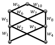
As an example, let us consider a simple 3 layer network with 2 nodes in each layer except for the output layer, which has only 1 node (see Figure 2). The network has 10 parameters (4, 4, and 2 in each layer respectively) and 8 paths. The Jacobian $(\partial f_{{\mathbf{w}}}({\mathbf{x}})/\partial{\mathbf{w}})$ can be written as $(\partial f_{{\mathbf{w}}}({\mathbf{x}})/\partial{\mathbf{w}})=J({\mathbf{w}})^{\top}\cdot\bm{\phi}({\mathbf{x}})$, where

$$J({\mathbf{w}}) =\left[\begin{array}[]{c|c|c}\begin{array}[]{cccc}w_{5}w_{9}&&&\\ &w_{5}w_{9}&&\\ &&w_{6}w_{9}&\\ &&&w_{6}w_{9}\\ \hline\cr w_{7}w_{10}&&&\\ &w_{7}w_{10}&&\\ &&w_{8}w_{10}&\\ &&&w_{8}w_{10}\\ \end{array}&\begin{array}[]{cccc}w_{9}w_{1}&&&\\ w_{9}w_{2}&&&\\ &w_{9}w_{3}&&\\ &w_{9}w_{4}&&\\ \hline\cr&&w_{10}w_{1}&\\ &&w_{10}w_{2}&\\ &&&w_{10}w_{3}\\ &&&w_{10}w_{4}\end{array}&\begin{array}[]{cc}w_{5}w_{1}&\\ w_{5}w_{2}&\\ w_{6}w_{3}&\\ w_{6}w_{4}&\\ \hline\cr&w_{7}w_{1}\\ &w_{7}w_{2}\\ &w_{8}w_{3}\\ &w_{8}w_{4}\end{array}\end{array}\right]$$ (50)

and

$$\phi({\mathbf{x}})^{\top} =\begin{bmatrix}g_{1}({\mathbf{x}})x[1]&g_{2}({\mathbf{x}})x[2]&g_{3}({\mathbf{x}})x[1]&g_{4}({\mathbf{x}})x[2]&g_{5}({\mathbf{x}})x[1]&g_{6}({\mathbf{x}})x[2]&g_{7}({\mathbf{x}})x[1]&g_{8}({\mathbf{x}})x[2]\end{bmatrix}.$$

The rank of $J({\mathbf{w}})$ in (50) is (generically) equal to $10-4=6$, which is smaller than both the number of parameters and the number of paths.

Figure 2: A 3 layer network with 10 parameters and 8 paths.

8 Conclusion and Future Work

We proposed a unified framework as a complexity measure or regularizer for neural networks and discussed normalization and optimization with respect to this regularizer. We further showed how this measure interpolates between data-dependent and data-independent regularizers and discussed how Path-SGD and Batch-Normalization are special cases of optimization with respect to this measure. We also looked at the issue of invariances and brought new insights to this area.

Appendix A Implementation

A.1 DDP-Normalization

Given any batch of $n$ data points to estimate mean, variance and the gradient, the stochastic gradients for the weight $\tilde{\mathbf{w}}$ (weights in the DDP-Normalized network) can then be calculated through the chain rule:

$$\frac{\partial L}{\partial\tilde{\mathbf{w}}_{\rightarrow v}} =\frac{1}{n\tilde{\gamma}_{v}}\sum_{i=1}^{n}\frac{\partial L}{\partial z_{v}^{(i)}}\left[{\mathbf{h}}_{N^{\text{in}}(v)}^{(i)}-\frac{1}{n}\sum_{j=1}^{n}{\mathbf{h}}_{N^{\text{in}}(v)}^{(j)}-\frac{\hat{z}^{(i)}_{v}}{2\tilde{\gamma}_{v}^{2}}\frac{\partial\tilde{\gamma}^{2}_{v}}{\partial\tilde{\mathbf{w}}_{\rightarrow v}}\right]$$ (51)

$$\frac{\partial L}{\partial z^{(i)}_{u}} =\frac{1}{\tilde{\gamma}_{v}}\left[\sum_{v\in N^{\text{out}}(u)}\tilde{w}_{u\rightarrow v}\left(\frac{\partial L}{\partial z_{v}^{(i)}}-\frac{1}{n}\sum_{j=1}^{n}\frac{\partial L}{\partial z_{v}^{(j)}}\left(1-\alpha\frac{\hat{z}^{(i)}_{v}\hat{z}^{(j)}_{v}}{\tilde{\gamma}^{2}_{v}}\right)\right)\right]_{z^{(i)}_{u}\geq 0}$$ (52)

where $\hat{z}^{(i)}_{v}=\tilde{z}^{(i)}_{v}-\frac{1}{n}\sum_{j=1}^{n}\tilde{z}^{(j)}_{v}$ and we have:

$$\frac{\partial\tilde{\gamma}^{2}_{v}}{\partial\tilde{\mathbf{w}}_{\rightarrow v}}=2(1-\alpha)\tilde{\mathbf{w}}_{\rightarrow v}+\frac{2\alpha}{n}\sum_{i=1}^{n}\hat{z}^{(i)}_{v}\left({\mathbf{h}}_{N^{\text{in}}(v)}^{(i)}-\frac{1}{n}\sum_{j=1}^{n}{\mathbf{h}}_{N^{\text{in}}(v)}^{(j)}\right)$$ (53)

Similar to Batch-Normalization, all the above calculations can be efficiently carried out as vector operations with negligible extra memory and computations.

A.2 DDP-SGD

In order to compute the second derivatives $\kappa_{e}(\mathbf{w})=\frac{\partial^{2}\gamma^{2}_{\rm net}}{\partial w^{2}_{e}}$, we first calculate the first derivative. The backpropagation can be done through $\gamma^{2}_{u}$ and $z^{(i)}_{u}$ but this makes it difficult to find the second derivatives. Instead we propagate the loss through $\gamma^{2}_{u}$ and the second order terms of the form $z^{(i)}_{u_{1}}z^{(i)}_{u_{2}}$:

$$\frac{\partial\gamma^{2}_{{\rm net}}}{\partial\gamma^{2}_{u}} =(1-\alpha)\sum_{v\in N^{\text{out}}(u)}\frac{\partial\gamma^{2}_{{\rm net}}}{\partial\gamma^{2}_{v}}w^{2}_{u\rightarrow v}$$ (54)

$$\frac{\partial\gamma^{2}_{{\rm net}}}{\partial(z_{u_{1}}^{(i)}z_{u_{2}}^{(i)})}=\alpha\left[\frac{\partial\gamma^{2}_{\rm net}}{\partial\gamma^{2}_{u_{1}}}\right]_{u_{1}=u_{2}}+\left[\sum_{(v_{1},v_{2})\in\left(N^{\text{out}}(u_{1})\right)^{2}}\frac{\partial\gamma^{2}_{\rm net}}{\partial(z_{v_{1}}^{(i)}z_{v_{2}}^{(i)})}w_{u_{1}\rightarrow v_{1}}w_{u_{2}\rightarrow v_{2}}\right]_{z^{(i)}_{u_{1}}>0,z^{(i)}_{u_{2}}>0}$$ (55)

Now we can calculate the partials for $w_{u\rightarrow v}$ as follows:

$$\frac{\partial\gamma^{2}_{\rm net}}{\partial w_{u\rightarrow v}}=2(1-\alpha)\frac{\partial\gamma^{2}_{\rm net}}{\partial\gamma^{2}_{v}}\gamma^{2}_{u}w_{u\rightarrow v}+2\sum_{i=1}^{n}\sum_{v^{\prime}\in N^{\text{out}}(u)}\frac{\partial\gamma^{2}_{\rm net}}{\partial(z^{(i)}_{v}z^{(i)}_{v^{\prime}})}h_{u}^{(i)}z_{v^{\prime}}^{(i)}$$ (56)

Since the partials $\frac{\partial\gamma^{2}_{{\rm net}}}{\partial\gamma^{2}_{u}}$ and $\frac{\partial\gamma^{2}_{{\rm net}}}{\partial(z_{u_{1}}^{(i)}z_{u_{2}}^{(i)})}$ do not depend on $w_{u\rightarrow v}$, the second order derivative can be calculated directly:

$$\kappa_{u\rightarrow v}(\mathbf{w})=\frac{1}{2}\frac{\partial^{2}\gamma^{2}_{\rm net}}{\partial w_{u\rightarrow v}^{2}}=(1-\alpha)\frac{\partial\gamma^{2}_{\rm net}}{\partial\gamma^{2}_{v}}\gamma^{2}_{u}+\sum_{i=1}^{n}\frac{\partial\gamma^{2}_{\rm net}}{\partial\left({z^{(i)}_{v}}^{2}\right)}\left(h^{(i)}_{u}\right)^{2}$$ (57)

Appendix B Natural Gradient

The natural gradient algorithm (Amari, 1998) achieves invariance by applying the inverse of the Fisher information matrix $F({\mathbf{w}}^{(t)})$ at the current parameter ${\mathbf{w}}^{(t)}$ to the negative gradient direction as follows:

$${\mathbf{w}}^{(t+1)} ={\mathbf{w}}^{(t)}+\eta\bm{\Delta}^{(\rm natural)},$$

where

$$\Delta^{(\rm natural)} =\underset{\Delta\in\mathbb{R}^{|E|}}{\mathrm{argmin}}\>\left\langle-\frac{\partial L}{\partial w}({\mathbf{w}}^{(t)}),\bm{\Delta}\right\rangle,\quad{\rm s.t.}\quad\bm{\Delta}^{\top}F({\mathbf{w}}^{(t)})\bm{\Delta}\leq\delta^{2}$$ (58)

$$=-F^{-1}({\mathbf{w}}^{(t)})\frac{\partial L}{\partial w}({\mathbf{w}}^{(t)}).$$ (59)

Here $F({\mathbf{w}})$ is the Fisher information matrix at point ${\mathbf{w}}$ and is defined with respect to the probabilistic view of the feedforward neural network model, which we describe in more detail below.

Suppose that we are solving a classification problem and the final layer of the network is fed into a softmax layer that determines the probability of candidate classes given the input $x$. Then the neural network with the softmax layer can be viewed as a conditional probability distribution

$$q(y|{\mathbf{x}})=\frac{\exp(f_{\mathbf{w}}({\mathbf{x}})[v_{y}])}{\sum_{v\in V_{\rm out}}\exp(f_{\mathbf{w}}({\mathbf{x}})[v])},$$ (60)

where $v_{y}$ is the output node corresponding to class $y$. If we are solving a regression problem a Gaussian distribution is probably more appropriate for $q(y|{\mathbf{x}})$.

Given the conditional probability distribution $q(y|{\mathbf{x}})$, the Fisher information matrix can be defined as follows:

$$F({\mathbf{w}})[e,e^{\prime}]=\mathbb{E}_{{\mathbf{x}}\sim p(\mathbf{x})}\mathbb{E}_{y\sim q(y|{\mathbf{x}})}\left[\frac{\partial\log q(y|{\mathbf{x}})}{\partial w_{e}}\frac{\partial\log q(y|{\mathbf{x}})}{\partial w_{e^{\prime}}}\right],$$ (61)

where $p(x)$ is the marginal distribution of the data.

Since we have

$$\frac{\partial\log q(y|{\mathbf{x}})}{\partial w_{u\rightarrow v}}=\frac{\partial\log q(y|{\mathbf{x}})}{\partial z_{v}}\cdot h_{u}=\sum_{v^{\prime}\in V_{\rm out}}\frac{\partial\log q(y|{\mathbf{x}})}{\partial z_{v^{\prime}}}\cdot\frac{\partial z_{v^{\prime}}}{\partial z_{v}}\cdot h_{u}$$ (62)

using the chain rule, each entry of the Fisher information matrix can be computed efficiently by forward and backward propagations on a minibatch.

Appendix C Proofs

Proof of Theorem 1.

First note that we can calculate the following inner product using equation (53):

$$\left\langle\tilde{\mathbf{w}}_{\rightarrow v},\frac{\partial\tilde{\gamma}_{v}^{2}}{\partial\tilde{\mathbf{w}}_{\rightarrow v}}\right\rangle =2(1-\alpha)\left\lVert{\tilde{\mathbf{w}}_{\rightarrow v}}\right\rVert_{2}^{2}+\frac{2\alpha}{n}\sum_{i=1}^{n}(\hat{z}^{(i)})^{2}$$

$$=2(1-\alpha)\left\lVert{\tilde{\mathbf{w}}_{\rightarrow v}}\right\rVert_{2}^{2}+2\alpha\text{Var}(\tilde{z}_{v})=2\tilde{\gamma}_{v}^{2}$$

Next, by equation (51) we get:

$$\left\langle\tilde{\mathbf{w}}_{\rightarrow v},\frac{\partial L}{\partial\tilde{\mathbf{w}}_{\rightarrow v}}\right\rangle =\frac{1}{n\tilde{\gamma}_{v}}\sum_{i=1}^{n}\frac{\partial L}{\partial z_{v}^{(i)}}\left[\hat{z}^{(i)}_{v}-\frac{\hat{z}^{(i)}_{v}}{2\tilde{\gamma}_{v}^{2}}\left\langle\tilde{\mathbf{w}}_{\rightarrow v},\frac{\partial\tilde{\gamma}^{2}_{v}}{\partial\tilde{\mathbf{w}}_{\rightarrow v}}\right\rangle\right]$$

$$=\frac{1}{n\tilde{\gamma}_{v}}\sum_{i=1}^{n}\frac{\partial L}{\partial z_{v}^{(i)}}\left[\hat{z}^{(i)}_{v}-\frac{\hat{z}^{(i)}_{v}}{2\tilde{\gamma}_{v}^{2}}2\tilde{\gamma}^{2}_{v}\right]=0$$

∎

Proof of Theorem 3.

First we see that (24) is true because

$$\frac{\partial f_{{\mathbf{w}}}({\mathbf{x}})[v]}{\partial{\mathbf{w}}}=\Bigl{(}\sum_{p\in\Pi(v)}\frac{\partial\pi_{p}({\mathbf{w}})}{\partial w_{e}}\cdot g_{p}({\mathbf{x}})\cdot x[{\rm head}(p)]\Bigr{)}_{e\in E}=J_{v}({\mathbf{w}})^{\top}\cdot\phi_{v}({\mathbf{x}}).$$

Therefore,

$$\bigcup_{{\mathbf{x}}\in\mathbb{R}^{|V_{\rm in}|}}{\rm Span}\left(\frac{\partial f_{{\mathbf{w}}}({\mathbf{x}})[v]}{\partial{\mathbf{w}}}:v\in V_{\rm out}\right) =\bigcup_{{\mathbf{x}}\in\mathbb{R}^{|V_{\rm in}|}}{\rm Span}\left(J_{v}({\mathbf{w}})^{\top}\cdot\phi_{v}({\mathbf{x}}):v\in V_{\rm out}\right)$$

$$=J({\mathbf{w}})^{\top}\cdot{\rm Span}\left(\phi({\mathbf{x}}):{\mathbf{x}}\in\mathbb{R}^{|V_{\rm in}|}\right).$$ (63)

Consequently, any vector of the form $(\frac{\partial f_{{\mathbf{w}}}({\mathbf{x}})[v]}{\partial w_{e}})_{e\in E}$ for a fixed input ${\mathbf{x}}$ lies in the span of the row vectors of the path Jacobian $J({\mathbf{x}})$.

The second part says $d_{G}({\mathbf{w}})={\rm rank}J({\mathbf{w}})$ if ${\rm dim}\left({\rm Span}(\phi({\mathbf{x}}):{\mathbf{x}}\in\mathbb{R}^{|V_{\rm in}|})\right)=|\Pi|$, which is the number of rows of $J({\mathbf{w}})$. We can see that this is true from expression (63).

∎

Proof of Theorem 4.

First, $J({\mathbf{w}})$ can be written as an Hadamard product between path incidence matrix $M$ and a rank-one matrix as follows:

$$J({\mathbf{w}}) =M\circ\left({\mathbf{w}}^{-1}\cdot\bm{\pi}^{\top}({\mathbf{w}})\right),$$

where $M$ is the path incidence matrix whose $i,j$ entry is one if the $i$th edge is part of the $j$th path, ${\mathbf{w}}^{-1}$ is an entry-wise inverse of the parameter vector ${\mathbf{w}}$, $\bm{\pi}({\mathbf{w}})=(\pi_{p}({\mathbf{w}}))$ is a vector containing the product along each path in each entry, and $\top$ denotes transpose.

Since we can rewrite

$$J({\mathbf{w}}) ={\rm diag}({\mathbf{w}}^{-1})\cdot M\cdot{\rm diag}(\bm{\pi}({\mathbf{w}})),$$

we see that (generically) the rank of $J({\mathbf{w}})$ is equal to the rank of zero-one matrix $M$.

Note that the rank of $M$ is equal to the number of linearly independent columns of $M$, in other words, the number of linearly independent paths. In general, most paths are not independent. For example, in Figure 2, we can see that the column corresponding to the path $w_{2}w_{7}w_{10}$ can be produced by combining 3 columns corresponding to paths $w_{1}w_{5}w_{9}$, $w_{1}w_{7}w_{10}$, and $w_{2}w_{5}w_{9}$.

In order to count the number of independent paths, we use mathematical induction. For simplicity, consider a layered graph with $d$ layers. All the edges from the $(d-1)$th layer nodes to the output layer nodes are linearly independent, because they correspond to different parameters. So far we have $n_{d}n_{d-1}$ independent paths.

Next, take one node $u_{0}$ (e.g., the leftmost node) from the $(d-2)$th layer. All the paths starting from this node through the layers above are linearly independent. However, other nodes in this layer only contributes linearly to the number of independent paths. This is the case because we can take an edge $(u,v)$, where $u$ is one of the remaining $n_{d-2}-1$ vertices in the $(d-2)$th layer and $v$ is one of the $n_{d-1}$ nodes in the $(d-1)$th layer, and we can take any path (say $p_{0}$) from there to the top layer. Then this is the only independent path that uses the edge $(u,v)$, because any other combination of edge $(u,v)$ and path $p$ from $v$ to the top layer can be produced as follows (see Figure 3):

$$(u,v)\rightarrow p=(u,v)\rightarrow p_{0}-(u_{0},v)\rightarrow p_{0}+(u_{0},v)\rightarrow p.$$

Therefore after considering all nodes in the $d-2$th layer, we have

$$n_{d}n_{d-1}+n_{d-1}(n_{d-2}-1)$$

independent paths. Doing this calculation inductively, we have

$$n_{d}n_{d-1}+n_{d-1}(n_{d-2}-1)+\cdots+n_{1}(n_{0}-1)$$

independent paths, where $n_{0}$ is the number of input units. This number is clearly equal to the number of parameters ($n_{d}n_{d-1}+\cdots+n_{1}n_{0}$) minus the number of internal nodes ($n_{d-1}+\cdots+n_{1}$). ∎

Figure 3: Schematic illustration of the linear dependence of the four paths $(u_{0},v)\rightarrow p_{0}$, $(u_{0},v)\rightarrow p$, $(u,v)\rightarrow p_{0}$, and $(u,v)\rightarrow p$. Because of this dependence, any additional edge $(u,v)$ only contributes one additional independent path.

References

- Amari (1998) Amari, Shun-Ichi. Natural gradient works efficiently in learning. Neural computation, 10(2):251–276, 1998.
- Desjardins et al. (2015) Desjardins, Guillaume, Simonyan, Karen, Pascanu, Razvan, and Kavukcuoglu, Koray. Natural neural networks. arXiv preprint arXiv:1507.00210, 2015.
- Glorot & Bengio (2010) Glorot, Xavier and Bengio, Yoshua. Understanding the difficulty of training deep feedforward neural networks. In AISTATS, 2010.
- Grosse & Salakhudinov (2015) Grosse, Roger and Salakhudinov, Ruslan. Scaling up natural gradient by sparsely factorizing the inverse Fisher matrix. In ICML, 2015.
- Ioffe & Szegedy (2015) Ioffe, Sergey and Szegedy, Christian. Batch normalization: Accelerating deep network training by reducing internal covariate shift. In ICML, 2015.
- Larochelle et al. (2009) Larochelle, Hugo, Bengio, Yoshua, Louradour, Jérôme, and Lamblin, Pascal. Exploring strategies for training deep neural networks. The Journal of Machine Learning Research, 10:1–40, 2009.
- Le Cun et al. (1998) Le Cun, Yann, Bottou, Léon, Orr, Genevieve B., and Müller, Klaus-Robert. Efficient backprop. In Neural Networks, Tricks of the Trade, Lecture Notes in Computer Science LNCS 1524. Springer Verlag, 1998. URL http://leon.bottou.org/papers/lecun-98x.
- LeCun et al. (1998) LeCun, Yann, Bottou, Leon, Orr, Genevieve B, and Muller, Klaus-Robert. Neural networks-tricks of the trade. Springer Lecture Notes in Computer Sciences, 1524(5-50):7, 1998.
- Martens (2010) Martens, James. Deep learning via hessian-free optimization. In ICML, 2010.
- Martens & Grosse (2015) Martens, James and Grosse, Roger. Optimizing neural networks with Kronecker-factored approximate curvature. In ICML, 2015.
- Neyshabur et al. (2015a) Neyshabur, Behnam, Salakhutdinov, Ruslan, and Srebro, Nathan. Path-SGD: Path-normalized optimization in deep neural networks. In NIPS, 2015a.
- Neyshabur et al. (2015b) Neyshabur, Behnam, Tomioka, Ryota, and Srebro, Nathan. Norm-based capacity control in neural networks. In COLT, 2015b.
- Neyshabur et al. (2015c) Neyshabur, Behnam, Tomioka, Ryota, and Srebro, Nathan. In search of the real inductive bias: On the role of implicit regularization in deep learning. International Conference on Learning Representations (ICLR) workshop track, 2015c.
- Ollivier (2015) Ollivier, Yann. Riemannian metrics for neural networks i: feedforward networks. Information and Inference, 4(2):108–153, 2015.
- Pascanu & Bengio (2014) Pascanu, Razvan and Bengio, Yoshua. Revisiting natural gradient for deep networks. In ICLR, 2014.
- Roux et al. (2008) Roux, Nicolas L, Manzagol, Pierre-Antoine, and Bengio, Yoshua. Topmoumoute online natural gradient algorithm. In NIPS, 2008.
- Schaul et al. (2013) Schaul, Tom, Zhang, Sixin, and Lecun, Yann. No more pesky learning rates. In ICML, 2013.
- Sutskever et al. (2013) Sutskever, Ilya, Martens, James, Dahl, George, and Hinton, Geoffrey. On the importance of initialization and momentum in deep learning. In ICML, 2013.
- Vinyals & Povey (2011) Vinyals, Oriol and Povey, Daniel. Krylov subspace descent for deep learning. In ICML, 2011.