Energy density profile inspired by noncommutativity

Abstract

An important consequence which comes from noncommutativity (NC) is undoubtedly the energy density characterized by a microscopic free parameter; indeed a Trans-Planckian parameter. However, its functional form is an interesting and useful equation which can be analyzed in astrophysical scenarios giving now astrophysical constraints. In this sense, this paper is devoted to explore the astrophysical consequences of an energy density with the same functional form of NC; mainly in stellar dynamics and rotation curves of galaxies. We start exploring toy models of stars with incompressible and polytropic fluids respectively, with the addition and coexistence with this new fluid. In both cases, we propose an appropriate constriction based on the difference between a correct and an anomalous behavior. As a complement, we explore the rotation curves of galaxies assuming that the halo is a fluid with the same characteristic of a NC equation, obtaining the range of values for the free parameter through the analysis of eighteen LSB galaxies. Our results are compared with traditional models studied in literature like Pseudoisothermal (PISO), Navarro-Frenk-White (NFW), Burkert and WaveDM dark matter models. Finally, we have computed the surface density, $\rho_{i}r_{i}$ for each dark matter model, where $i$ is for PISO, NFW, Burkert, WaveDM and NC macroscopic version. In the later case, following the results found using SPARC galaxy catalog, we have found a theoretical value of $116.97M_{\odot}$ pc^-2 while the data analysis gives us a value of $144.21M_{\odot}$ pc^-2. The values of the surface density $\rho_{i}r_{i}$ are roughly constant and their mean values depend on the dark matter model. Also we have computed the mass of each dark matter model within $300$ pc and found that there is a common mass for spiral galaxies of the order of $10^{7}M_{\odot}$, that is in agreement with the results for dSph Milky Way satellites. This would give a central density for the halo of $\sim 0.1M_{\odot}$ pc^-2 independent of the dark matter model.

I Introduction

One of the most successful outcomes of string theory is that the space-time coordinates may become NC operators and lead us to a NC version of a gauge theory via the Seiberg and Witten map Seiberg and Witten (1999). After this result was published, a large number of papers related with NC in gauge theories, quantum mechanics, classical mechanics, quantum field theory and gravity has been published. In addition it is possible to note that the NC parameter has been bounded by different observations or experiments, mainly leading to an extremely small value Romero and Vergara (2003).

A different NC formulation of quantum field theory, based on coherent state formulation, can be achieved using the Feynman path integral on the NC plane which is a used framework for quantum mechanics and field theory Nicolini et al. (2006). In a recent paper Smailagic and Spallucci (2003) the authors discuss the gravitational analogue of the NC modification of quantum field theory, pointing out that NC is an intrinsic property of the manifold itself and affects gravity in an indirect way. The energy-momentum density determines space-time curvature. Thus in General Relativity (GR), the effects of NC can be taken into account by keeping the standard form of Einstein curvature tensor and introducing a modified energy-momentum tensor. The NC eliminates the point-like structures and replace them by smeared objects. The effect of smearing is implemented by using a Gaussian distribution of minimal width $\sqrt{\gamma}$ instead of a Dirac-delta function where the spherically symmetric and particle-like gravitational source can be written as:

$$\rho_{\gamma}(r)=\frac{M_{NC}}{(4\pi\gamma)^{3/2}}\exp\left(-\frac{r^{2}}{4\gamma}\right),$$ (1)

where $M_{NC}$ is the total mass parameter and $\gamma$ the NC parameter of the energy density related with the smearing of the NC energy density distribution. In traditional literature, NC free parameter has only been studied in quantum scenarios, constraining the value at Trans-Planckian scales Alboteanu et al. (2006); Mohammadi Najafabadi (2006); He and Li (2006), only having important effects in quantum gravity theories.

Hence, in order to study large scales, we relate the following functions and we change the NC parameter which comes from a quantum theory for a new macroscopic parameter $\theta$, applicable to astrophysical issues, following the recipe:

$$\rho_{\gamma}(r)\to\rho_{\theta}(r),\;\;M_{NC}\to M_{NED}\;\;\rm and\;\;\gamma\to\theta.$$ (2)

The parameter are constrained by observations or under arguments of a behavior that fits with the the traditional literature. Indeed, if we assume that this fluid permeates the galaxies structures, it is natural to study the presence of this fluid, also in the stellar dynamics.

Therefore, to start the study we will call this new fluid as noncommutativity energy density (NED) for the inspiration that comes from NC; then we give ourselves to the task of study the previous statements, proposing two exercises to analyze the dynamics in a scenario where baryons and NED coexist (without mutual interaction), i.e. $T_{\mu\nu}^{eff}=T_{\mu\nu}^{bar}+T_{\mu\nu}^{NED}$, where the first one is related with the baryonic matter and the second one is related with NED, producing the astrophysical dynamics observed and with this, constraint the NED parameter with observables. These two exercises analyze the new dynamic produced by the presence of NED, mainly in the evolution and dynamic of the stars and in rotation curves of galaxies.

In this sense, there has been extensive studies in stellar dynamics since the advent of GR Weinberg (1972); in such a way that observing the imprints of NED in the dynamics must be clear, showing deviations to GR predictions. For instance it is possible to assume that hypothetical NED particles are so heavy, forming a dense core in the star center allowing the applied treatment in the following sections. In this vein, stars with uniform density and white dwarfs are studied due that are excellent laboratories to study possible extensions to the GR background. It is important to remark that extensive studies about NC, can be seen in Hernandez-Almada and Garcia-Aspeitia (2016).

In addition, the functional form of Eq. (1) with the recipe (2), inspire to be used as a density profile to reproduce the velocity rotation curves of galaxies, due to its similarity with Einasto’s model Einasto (1965) with $n^{\prime}=0.5$. In galactic dynamic the NED matter is concentrated mainly in the halo, with a Gaussian density profile and thus giving restrictions to the free parameter $\sqrt{\theta}$; constraining where NED parameter generates important effects. Other interesting dark matter (DM) proposals can be checked in Refs. Begeman et al. (1991); Navarro et al. (1997); Burkert (1995); Martins and Salucci (2007); Rodríguez-Meza (2012); Guzmán and Matos (2000) or for an excellent review see Ref. Sofue and Rubin (2001).

Recapitulating, we remark that the recipe shown in Eq. (2) as a macroscopic phenomena, will generate constraints of the $\theta$ parameter also, of the order of macroscopic scales. This of course contributes to generate a macroscopic bounds, which was left out by Ref. Rahaman et al. (2012), contributing to strengthen these previous research. In this sense, we will provide a table of the constraints of this parameter, which will be subject to the theoretical model under study or the observations with which it is contrasted.

From here, it is possible to organize the paper as follows: In Sec. II, we analyze a Newtonian star in two cases, where it is composed by an uniform density (incompressible fluid) coexisting with the NED matter and when it is composed by a polytropic matter and the core contains a NED fluid, showing a modified Lane-Emden equation, constraining the NED free parameter and fixing the NED mass as a subdominant component. In Sec. III we implement an analysis of galactic rotation curves, assuming that the DM halo can be modeled by NED density matter. In this case, we use a sample of eighteen LSB galaxies without photometry with the aim of constraint the NED parameters ($\rho_{NED}$ and $\sqrt{\theta}$) and compare with traditional density profile models like pseudoisothermal (PISO), Navarro-Frenk-White (NFW), Burkert and the WaveDM studied in these two Refs.Ureña-López et al. (2017); Bernal et al. (2017), it is an ultralight scalar model motivated by large scale simulationsSchive et al. (2014). Finally in Sec. IV we give a discussion and conclusions about the results obtained through the paper.

In what follows, we work in units in which $c=\hbar=1$, unless explicitly written.

II Toy model stars with a NED component

In this section, we study the stellar dynamics with a component of NED, together with the traditional baryonic matter. We start using the approach of a Newtonian star, composed by this fluid and baryonic matter with uniform density (incompressible fluid). After that, we study a most generic star through the Lane-Emden (LE) equation, under the assumption that the star is composed by a polytrope and also contains a NED. Both models are considered under the premise that ordinary matter does not interact with the NED and fixes one of the free parameters, with the argument of a subdominant NED.

II.1 NED matter on stars with uniform density in Newtonian approach

These stars are of interest, because they are simple enough to allow an exact solution in Newtonian background. Then, stars with uniform density consist of an incompressible fluid with equation of state (EoS), $\rho_{I}=\rm constant$, in such a way that a generalization with the addition of NED is simple, being excellent laboratories to understand the physics behind such processes.

In a Newtonian approach, dynamic equation for the evolution of a star can be written as:

$$r^{2}\frac{dp(r)}{dr}=-G\mathcal{M}(r)\rho_{eff}(r),$$ (3)

being $G$ the Newtonian gravitational constant, $\rho_{eff}(r)$ the effective density and $\mathcal{M}(r)$ the stellar mass written in the form:

$$\mathcal{M}(r)=4\pi\int_{0}^{r}r^{\prime 2}\rho_{eff}(r^{\prime})dr^{\prime}.$$ (4)

Eqs. (3) and (4) are considered as the equations of motion for stellar dynamics in Newtonian approach. In addition, we propose that the star density is composed by an uniform component density and a NED in the following form:

$$\rho_{eff}(r)=\rho_{I}+\frac{M_{NED}}{(4\pi\theta)^{3/2}}\exp\left(-\frac{r^{2}}{4\theta}\right),$$ (5)

where $\rho_{I}$ is a constant and there is not mutual interaction between the components. In order to have a numerical solution of the equations of motion we assume the following dimensionless variables:

$$x=\sqrt{\frac{GM}{R}}\left(\frac{r}{R}\right),\;\;\bar{\mathcal{M}}(r)=\sqrt{\frac{G^{3}M}{R^{3}}}\mathcal{M}(r),\;\;$$ (6a)

$$\bar{p}(r)=\frac{4\pi R^{3}}{M}p(r),\;\bar{\theta}=\frac{4GM}{R^{3}}\theta,\;\;\bar{\rho}_{I}=\frac{4\pi R^{3}}{3M}\rho_{I},\;\;$$ (6b)

$$\bar{M}^{NED}=8\sqrt{\frac{G^{3}M}{\pi R^{3}}}M_{NED},$$ (6c)

and integrating Eq. (4) we have:

$$\bar{\mathcal{M}}(x)=\bar{\rho}_{I}x^{3}+$$

$$\frac{\bar{M}^{NED}}{\bar{\theta}^{3/2}}\left[\sqrt{\pi}\left(\frac{\bar{\theta}}{4}\right)^{3/2}{\rm Erf}\left(\frac{x}{\sqrt{\bar{\theta}}}\right)-\frac{\bar{\theta}}{4}x\exp\left(-\frac{x^{2}}{\bar{\theta}}\right)\right]\,\,,$$ (7)

where $\rm Erf(x)$ is the error function defined as: ${\rm Erf}(x)=(2/\sqrt{\pi})\int_{0}^{x}\exp(-t^{2})dt$.

The behavior can be seen in Fig. 1 (Top) for different values of $\bar{\theta}$. In this case, we propose the extreme case for the free parameters in the form: $\bar{\rho}_{I}=0.9$ and $\bar{M}^{NED}=0.1$, considering domination of baryonic matter over NED component. It is important to mention that a greater amount of NED material, compromises the stability of the star.

Also, we analyze an extreme Newtonian star fulfilling the compactness relation $GM/R=0.44$. Indeed, it is possible to observe that the dimensionless NED parameter $\bar{\theta}$ dictates the behavior of the stellar mass.

In addition, Eq. (3) can be written in terms of dimensionless variables as:

$$\frac{d\bar{p}(x)}{dx}=-\frac{\bar{\mathcal{M}}(x)}{x^{2}}\left[3\bar{\rho}_{I}+\frac{\bar{M}^{NED}}{\bar{2\theta}^{3/2}}\exp\left(-\frac{x^{2}}{\bar{\theta}}\right)\right],$$ (8)

and its numerical integration can be observed in Fig. 1 (Bottom) for different values of the NED parameter. It is notorious how for values below $\bar{\theta}=10^{-1}$, pressure and mass present important differences in comparison with the other cases when the NED parameter plays a role.

Thus, small values of NED parameter shown the convergence to the traditional behavior without NED for pressure and mass in a Newtonian star with uniform density.

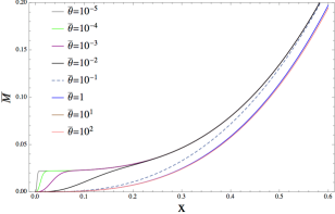
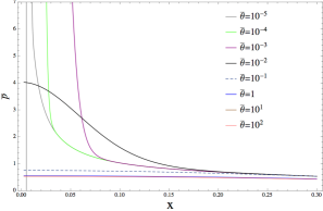
Figure 1: Behavior of $\bar{\mathcal{M}}$ and $\bar{p}$ vs $x$, assuming the following free parameters: $\bar{\rho}_{B}=0.9$, $\bar{M}^{NED}=0.1$ and $GM/R=0.44$; together with the initial condition $\bar{p}(0.663)=0$ for Eq. (8). (Top) In this case it is possible to note how mass shows almost the traditional behavior when $\bar{\theta}<1$, other upper values, present important contributions that comes from NED. (Bottom) Pressure behavior for different values of $\bar{\theta}$, blue line is the threshold between the standard behavior and the behavior when NED play an important role for an incompressible fluid.

From both results we conclude that it is necessary that $\bar{\theta}<1$ to obtain the traditional behavior found in literature (stars with only uniform density) for pressure and mass. Then, based on the results shown in Figs. 2 and with the aim of mimic the well known stellar behavior, it is possible to establish a bound of the NED parameter as:

$$\sqrt{\theta}<\frac{1}{2}\sqrt{\frac{R}{GM}}R,$$ (9)

where for a star in the limit of stellar stability as it is our case, we have $\sqrt{\theta}<0.753R$; which it is highly dependent on the stellar radius and the value must be macroscopic in order that fits to stellar dynamics.

II.2 Dwarf stars with NED

A dwarf star is mainly composed by a polytropic matter with equation of state (EoS) $P=K\rho^{(n+1)/n}$, being $K$ the polytropic constant and $n$ the polytropic index. This kind of stars are the most studied in literature due that it is possible to model them by just specifying the values of $K$ and $n$, having in mind the appropriate limits of both stellar structures.

However now we consider a NED component in the effective density of the star. Starting from Eq. (3) it is possible to write the modified LE equation as:

$$\frac{1}{\zeta^{2}}\frac{d}{d\zeta}\zeta^{2}\frac{d\Theta}{d\zeta}+\Theta^{n}=\frac{M^{0}_{NED}}{\bar{\theta}^{3/2}}\exp\left(-(1+n)\frac{\zeta^{2}}{\bar{\theta}}\right),$$ (10)

where it was proposed the following dimensionless variables:

$$r=\zeta\left(\frac{K(1+n)}{4\pi G}\right)^{1/2}\rho(0)^{(1-n)/2n},\rho=\rho(0)\Theta^{n},\;\;$$ (11a)

$$P=K\rho(0)^{(1+n)/n}\Theta^{n+1},\theta=\frac{K\rho(0)^{(1-n)/n}}{16\pi G}\bar{\theta},\;\;$$ (11b)

$$M_{NED}=\left(\frac{4\pi K\rho(0)^{(1-n)/n}}{16\pi G}\right)^{3/2}M^{0}_{NED}.$$ (11c)

Notice that $\rho(0)$ is the density at the center of the star. Moreover, we assume the same initial conditions for the problem of LE as: $\Theta(0)=1$, $\Theta^{\prime}(0)=0$ and in case of Dwarf stars, it is assumed a polytropic index $n=3$. The results are shown in Fig. 2, restricting a subdominant $M^{0}_{NED}=0.1$ and $\bar{\theta}$ is related with the presence of NED term in LE equation and being the two free parameters of the theory. Here, the results are more restrictive, showing that for values $10^{-4}\geqslant\bar{\theta}$ and $\bar{\theta}\geqslant 1$, it is recovered the traditional case. Therefore, using Eq. (11b), it is possible to constraint the NED parameter as

$$\kappa\geqslant 10^{2}\sqrt{\theta}\;\;\rm and\;\;\kappa\leqslant\sqrt{\theta},$$ (12)

where

$$\kappa\equiv\left[\frac{5}{192\pi^{3}G}\left(\frac{3\pi^{2}}{m_{N}\mu}\right)^{4/3}\frac{1}{\rho(0)^{2/3}}\right]^{1/2},$$ (13)

being $\mu$ the number of nucleons per electron, $m_{N}$ is the nucleon mass Weinberg (1972) and $\rho(0)$ is shown in Table 1 for different Dwarf Stars reported in literature Balberg and Shapiro (2000); Shipman et al. (1997); Holberg et al. (1998). Inside of the region, the NED presence is predominant and therefore, not having a traditional behavior of the stellar dynamics.

Also, we report the values of the NED parameters for the fifteen white dwarfs shown in Table 1, constraining the NED parameter with observables to obtain a traditional behavior shown in literature.

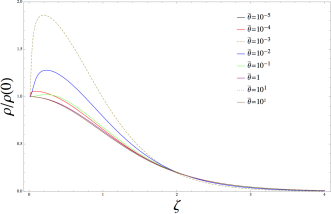
Figure 2: Behavior of $\Theta$ vs $\zeta$, with the initial conditions $\Theta(0)=1$, $\Theta^{\prime}(0)=0$. Top, from left to right and similarly from the figures in the bottom, we use $M^{0}_{NED}=0.1$.

White Dwarf sample
Observational data
White Dwarf	Mass (M⊙)	Radius (R⊙)	$\rho(0)$ (MeV4)	$\sqrt{\theta}$($10^{18}$MeV-1$\geqslant/\leqslant 10^{-2}$)
Sirius B	1.034	0.0084	10.5993	3.87583
Procyon B	0.604	0.0096	4.1478	5.29888
40 Eri B	0.501	0.0136	1.21009	7.98947
EG 50	0.50	0.0104	2.70063	6.11367
GD 140	0.79	0.0085	7.81565	4.29011
CD-38 10980	0.74	0.01245	2.3298	6.4222
W485A	0.59	0.0150	1.06212	8.34448
G154-B5B	0.46	0.0129	1.3006	7.79966
LP 347-6	0.56	0.0124	1.7827	7.02152
G181-B5B	0.54	0.0125	1.6781	7.16447
WD1550+130	0.535	0.0211	0.3456	12.132
Stein 2051B	0.48	0.0111	2.13023	6.6168
G107-70AB	0.65	0.0127	1.926	6.84287
L268-92	0.70	0.0149	1.28438	7.83236
G156-64	0.59	0.0110	2.69047	6.12135

Table 1: From left to right the columns read; name of the star, mass in solar units M_⊙, radius in R_⊙, density as $\rho(0)=3M/4\pi R^{3}$ in ${\rm MeV}^{4}$ and NED parameter in ${\rm MeV}^{-1}$ deduced from the constraint mentioned in text. Here we use a catalogue of fifteen white dwarfs reported in (Balberg and Shapiro, 2000; Shipman et al., 1997; Holberg et al., 1998).

III NED in galaxy rotation velocities

To complement our analysis we study rotation curves of galaxies at the weak gravitational field limit in order to study NED parameters. We start modeling the halo of the galaxy with the energy density of the NED shown in Eqs. (1) and (2).

Moreover, it is important to notice some important characteristics of NED profile. Implementing an appropriate series expansion of the NED of the order $r\ll\sqrt{\theta}$, we generate a functional form similar to PISO Begeman et al. (1991). In this context, this density profile is valid only at the center of galaxies. However, PISO density profile is an empirical profile designed for modeling DM in spirals galaxies and it has been applied not only at the center of galaxies but also in the outer spatial regions. Also, it is possible to observe that NED is a particular case of Einasto’s density profile Einasto (1965) (see Eq. (14)) when $n^{\prime}=0.5$

$$\rho_{Ein}=\rho_{-2}\exp\left(-2n^{\prime}\left[\left(\frac{r}{r_{-2}}\right)^{1/n^{\prime}}-1\right]\right),$$ (14)

where $r_{-2}$ is the radius where the density profile has a slope $-2$ and $\rho_{-2}$ is the local density at that radius; the parameter $n^{\prime}$ is known as Einasto index which describes the shape of the density profile.

In general, the NED distribution can provide with extra information than other models can not (see for example Begeman et al. (1991); Navarro et al. (1997); Burkert (1995)), mainly due to the advantage that comes naturally from the geometric properties of space-time and it is not just chosen by observations or numerical simulations.

On the other hand, we have that the rotation velocity is obtained from the absolute value of the effective potential as:

$$V^{2}(r)=r\left|\frac{d\Phi(r)}{dr}\right|=\frac{G\mathcal{M}(r)}{r},$$ (15)

where $\Phi(r)$ is the gravitational potential and $\mathcal{M}(r)$ is the total mass which describes the galactic dynamics and it is expressed in the same way as it is shown in Eq. (4) or as given in Eq. (19) for the mass, $M_{DM}(r)$, steaming for a dark matter (DM) distribution.

III.1 NED rotation velocity

The rotation velocity for the NED can be obtained through the NED distribution, giving the following relationship:

$$V^{2}_{\rm NED}(r) = \frac{4\pi G\theta^{3/2}\rho_{NED}}{r}$$ (16)

$$\times\left[\sqrt{\pi}{\rm Erf}\left(\frac{r}{2\sqrt{\theta}}\right)-\frac{r}{\sqrt{\theta}}\exp\left(-\frac{r^{2}}{4\theta}\right)\right],$$

where again, ${\rm Erf}(x)$ is the error function. This expression can be rewritten as

$$V^{2}_{\rm NED}(r)=4\pi G\sqrt{\theta}\,\mu_{DM}\hat{V}(r/2\sqrt{\theta})$$ (17)

where $\hat{V}(x)$ is a dimensionless function and we have defined $\mu_{DM}=\sqrt{\theta}\,\rho_{NED}$ (Eq. (21)), which has turned out to be a very important quantity, characterizing the dark matter models in galaxiesDonato et al. (2009). It has units of surface density. The rotation curve equations for PISO, NFW, Burkert and WaveDM models can also be written similarly as (17) (see Appendix A).

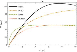
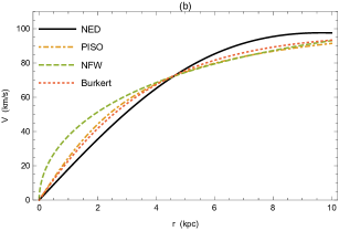
Figure 3: This figure shows a comparison of rotation curves for NED, PISO, NFW and Burkert models i.e. Eqs. (16), (24), (27) and (30). In (a) we plot all models with the same parameters values ($\mu_{DM}=92.47$ $M_{\odot}/$pc² and $r_{i}=2.5$ kpc, $i$ for each one of the models). In (b) we have chosen parameters values of NED, NFW and Burkert in order to the rotation curves almost resemble the one of PISO.

Let as first make a comparison of rotation curves associated with PISO, NFW and Burkert (See Appendix A) versus NED. Here we do not considere WaveDM model. The comparison between these three models and the NED rotation curves is shown in Fig. 3. In Fig. 3(a) we have plotted all the DM models with the same parameters values just to see their behavior. Given that $\mu_{DM}$ is the same for all the four models their different behavior came alone from the dimensionless function $\hat{V}(r/r_{i})$ times $r_{i}$, even do $r_{i}$ values are the same. In Fig. 3(b) we tried to reproduce almost the same behavior of the PISO rotation curve which has been produced with $\mu_{DM}=92.47$ $M_{\odot}/$pc² and $r_{p}=2.5$ kpc, by adjusting the parameters values of the other three models: NED: $\mu_{DM}=59.18$ $M_{\odot}/$pc² and $\sqrt{\theta}=3.2$ kpc; NFW: $\mu_{DM}=55.48$ $M_{\odot}/$pc² and $r_{n}=20$ kpc; and Burkert: $\mu_{DM}=166.45$ $M_{\odot}/$pc² and $r_{b}=4.8$ kpc. It has been found that $\mu_{DM}$ is almost constant for cored mass modelsDonato et al. (2009).

III.2 Constraints with LSB galaxies

The main goal of this section, is to compare the results of galaxy rotation curves, comparing the NED parameters fit with parameters fit given by the four most successful models studied in literature which are PISO, NFW, Burkert and WaveDM densities profiles (See Appendix A for details of the formulae used to fit observations).

In this sense, it is necessary to obtain the best fit, by maximizing the likelihood $\mathcal{L}(\Theta)\varpropto\exp[-\chi^{2}(\Theta)/2]$, where

$$\chi^{2}(\Theta)=\sum_{j=1}^{N}\left(\frac{V_{\rm obs}^{j}-V_{{\rm DM}}(r_{j},\Theta)}{\delta V_{{\rm obs}}^{j}}\right)^{2},$$ (18)

here $V^{i}_{\rm obs}$ and $\delta V^{i}_{\rm obs}$ is the observed velocity and its corresponding uncertainty at the observed radial distance $r_{j}$. $\Theta$ corresponds to the free parameters of DM model. The reduced $\chi^{2}$ is defined by $\chi^{2}_{\rm red}=\chi^{2}/(N-p)$ where $N$ is the total number of data and $p$ is the number of free parameters Press et al. (2007). Errors in the estimated parameters were computed using the covariance matrix as is described in Ref. Press et al. (2007).

For the DM models analyzed in this work we have two parameters: a scale length, $r_{i}$, and the density at the center of the galaxy, $\rho_{i}$; $i$ is for PISO, NFW, Burkert, WaveDM or NED models, Eqs. (22), (25), (28), (31) and (34). As we have already say, we defined in Eq. (21), the surface density, $\mu_{DM}$, which has turned out to be a very important quantity, characterizing the dark matter models in galaxies Donato et al. (2009).

Galaxy sample
Observational data
Galaxy	Morphology	$D$	$V_{\text{hel}}$	$M_{\text{abs}}(B)$	$R_{\text{max}}$	$V_{\text{max}}$
		(Mpc)	(km/s)	(mag)	(kpc)	(km/s)
(1)	(2)	(3)	(4)	(5)	(6)	(7)
(1) ESO 0140040	Spiral	212	16064	-21.6	29.2	263
(2) ESO 0840411	Edge-on	80	6200	-18.1	8.9	61
(3) ESO 1200211	Fuzzy Magellanic bar	15	1314	-15.6	3.5	25
(4) ESO 1870510	Irregular spiral, floculent	18	1410	-16.5	3.0	40
(5) ESO 2060140	Spiral	60	4704	-19.2	11.6	118
(6) ESO 3020120	Spiral, hint of bar?	69	5311	-19.1	11.0	86
(7) ESO 3050090	Barred spiral	11	1019	-17.3	4.8	54
(8) ESO 4250180	Spiral	86	6637	-20.5	14.4	145
(9) ESO 4880049	Inclined Magellanic bar	22	1800	-16.8	6.0	97
(10) F730-V1	Spiral	144	10714	-19.2	11.9	145
(11) UGC 4115	Fuzzy	3.2	343	-12.4	1.0	40
(12) UGC 11454	Fuzzy spiral, small core	91	6628	-18.6	11.9	152
(13) UGC 11557	Fuzzy spiral, small core	22	1390	-20.0	6.2	95
(14) UGC 11583	Faint Magellanic bar	5	128	-14.0	1.5	36
(15) UGC 11616	Fuzzy, irregular	73	5244	-20.3	9.6	143
(16) UGC 11648	Irregular	48	3350	-21.0	12.7	145
(17) UGC 11748	Irregular, bright core/bar?	73	5265	-22.9	21.0	242
(18) UGC 11819	Fuzzy	60	4261	-20.3	11.7	153

Table 2: Sample of LSB galaxies without photometry as given in Ref. de Blok et al. (2001). In column (1) we give the name of each galaxy; in column (2) we give the morphology of each galaxy; column (3) is the distance to the galaxy in Mpc; column (4) is the heliocentric systemic velocity; column (5) is the absolute magnitude in B-band of each galaxy; column (6) is distance in kpc where the maximum velocity is reach; column (7) is the maximum velocity of each rotation curve.

PISO DM Model
Best Fitting Parameters
Galaxy	$\rho_{p}$	$r_{p}$	$\mu_{DM}$	$M_{DM}(300$ pc$)$	$M_{DM}(r_{\text{max}})$	$\chi^{2}_{\text{red}}$
	($10^{-3}M_{\odot}/$pc3)	(kpc)	($M_{\odot}/$pc2)	($10^{7}M_{\odot}$)	($10^{11}M_{\odot}$)
(1)	(2)	(3)	(4)	(5)	(6)	(7)
(1) ESO 0140040	249.301$\pm$100.439	2.559$\pm$0.657	11.798	2.797	5.374	0.180
(2) ESO 0840411	5.235$\pm$2.031	6.376$\pm$3.308	0.617	0.059	0.087	0.050
(3) ESO 1200211	45.952$\pm$45.122	0.573$\pm$0.382	0.487	0.448	0.005	0.078
(4) ESO 1870510	54.231$\pm$29.375	0.967$\pm$0.448	0.970	0.580	0.012	0.028
(5) ESO 2060140	233.076$\pm$79.144	1.164$\pm$0.239	5.016	2.536	0.408	0.106
(6) ESO 3020120	54.204$\pm$26.987	1.895$\pm$0.707	1.900	0.604	0.216	0.034
(7) ESO 3050090	27.322$\pm$13.025	2.091$\pm$1.005	1.057	0.305	0.038	0.048
(8) ESO 4250180	30.192$\pm$37.443	4.398$\pm$4.190	2.456	0.341	0.686	0.095
(9) ESO 4880049	102.348$\pm$38.523	1.622$\pm$0.469	3.071	1.134	0.138	0.017
(10) F730-V1	214.024$\pm$69.305	1.472$\pm$0.304	5.828	2.362	0.587	0.083
(11) UGC 4115	149.748$\pm$63.661	0.931$\pm$0.765	2.579	1.595	0.004	0.004
(12) UGC 11454	151.154$\pm$29.156	1.926$\pm$0.246	5.385	1.685	0.668	0.382
(13) UGC 11557	15.453$\pm$6.272	5.378$\pm$3.683	1.537	0.174	0.093	0.051
(14) UGC 11583	119.175$\pm$72.692	0.633$\pm$0.355	1.394	1.191	0.005	0.106
(15) UGC 11616	199.314$\pm$43.504	1.498$\pm$0.223	5.521	2.201	0.431	0.171
(16) UGC 11648	105.879$\pm$19.255	1.948$\pm$0.235	3.814	1.181	0.511	3.739
(17) UGC 11748	8165.259$\pm$3307.033	0.367$\pm$0.078	55.482	67.067	2.857	5.719
(18) UGC 11819	88.880$\pm$14.071	2.933$\pm$0.387	4.821	0.999	0.769	0.316

Table 3: Best fitting parameters for PISO DM model and derived quantities.

NFW DM Model
Best Fitting Parameters
Galaxy	$\rho_{n}$	$r_{n}$	$\mu_{DM}$	$M_{DM}(300$ pc$)$	$M_{DM}(r_{\text{max}})$	$\chi^{2}_{\text{red}}$
	($10^{-3}M_{\odot}/$pc3)	(kpc)	($M_{\odot}/$pc2)	($10^{7}M_{\odot}$)	($10^{11}M_{\odot}$)
(1)	(2)	(3)	(4)	(5)	(6)	(7)
(1) ESO 0140040	25.478$\pm$11.506	16.148$\pm$4.602	7.609	22.701	5.392	0.142
(2) ESO 0840411	0.011$\pm$0.023	1157.493$\pm$2464.316	0.233	0.713	0.071	1.728
(3) ESO 1200211	2.419$\pm$5.244	5.705$\pm$9.200	0.255	0.729	0.006	0.239
(4) ESO 1870510	0.753$\pm$3.829	31.828$\pm$150.341	0.443	1.338	0.013	0.057
(5) ESO 2060140	19.886$\pm$9.262	8.110$\pm$2.327	2.983	8.688	0.415	0.420
(6) ESO 3020120	2.622$\pm$3.451	19.720$\pm$20.010	0.956	2.865	0.230	0.328
(7) ESO 3050090	3.153$\pm$2.380	10.000$\pm$5.829	0.583	1.714	0.029	0.654
(8) ESO 4250180	0.525$\pm$3.747	119.446$\pm$770.596	1.159	3.531	0.756	0.013
(9) ESO 4880049	10.366$\pm$6.610	10.000$\pm$4.634	1.917	5.635	0.130	0.608
(10) F730-V1	18.747$\pm$7.817	10.000$\pm$2.709	3.467	10.191	0.584	1.455
(11) UGC 4115	5.093$\pm$6.316	10.00$\pm$11.428	0.942	2.769	0.003	0.939
(12) UGC 11454	20.351$\pm$4.611	10.000$\pm$1.447	3.764	11.063	0.634	4.780
(13) UGC 11557	4.738$\pm$2.736	10.000$\pm$4.128	0.876	2.576	0.061	3.265
(14) UGC 11583	3.629$\pm$5.640	10.000$\pm$13.774	0.671	1.973	0.005	0.833
(15) UGC 11616	18.362$\pm$6.408	10.000$\pm$2.393	3.396	9.982	0.434	1.683
(16) UGC 11648	14.585$\pm$2.799	10.000$\pm$1.216	2.697	7.929	0.486	3.031
(17) UGC 11748	498.342$\pm$92.553	3.191$\pm$0.288	29.411	79.738	2.370	3.546
(18) UGC 11819	20.272$\pm$5.070	10.000$\pm$1.674	3.749	11.020	0.613	4.473

Table 4: Best fitting parameters for NFW dark matter model and derived quantities.

Burkert DM Model
Best Fitting Parameters
Galaxy	$\rho_{b}$	$r_{b}$	$\mu_{DM}$	$M_{DM}(300$ pc$)$	$M_{DM}(r_{\text{max}})$	$\chi^{2}_{\text{red}}$
	($10^{-3}M_{\odot}/$pc3)	(kpc)	($M_{\odot}/$pc2)	($10^{7}M_{\odot}$)	($10^{11}M_{\odot}$)
(1)	(2)	(3)	(4)	(5)	(6)	(7)
(1) ESO 0140040	174.894$\pm$37.361	5.973$\pm$0.807	19.320	1.903	4.811	0.556
(2) ESO 0840411	5.848$\pm$2.402	10.423$\pm$6.001	1.127	0.065	0.088	0.034
(3) ESO 1200211	47.651$\pm$39.331	1.010$\pm$0.529	0.890	0.420	0.005	0.070
(4) ESO 1870510	59.656$\pm$28.150	1.603$\pm$0.628	1.768	0.580	0.012	0.031
(5) ESO 2060140	190.003$\pm$46.654	2.480$\pm$0.336	8.713	1.954	0.363	0.193
(6) ESO 3020120	56.685$\pm$23.031	3.372$\pm$0.960	3.535	0.598	0.200	0.006
(7) ESO 3050090	30.689$\pm$14.441	3.376$\pm$1.581	1.916	0.324	0.038	0.042
(8) ESO 4250180	30.713$\pm$30.272	7.695$\pm$5.812	4.371	0.337	0.676	0.111
(9) ESO 4880049	110.947$\pm$37.263	2.729$\pm$0.669	5.599	1.151	0.133	0.046
(10) F730-V1	191.278$\pm$50.734	2.931$\pm$0.460	10.370	1.997	0.533	0.569
(11) UGC 4115	167.708$\pm$81.223	1.543$\pm$1.520	4.787	1.621	0.004	0.002
(12) UGC 11454	138.988$\pm$20.518	3.705$\pm$0.342	9.524	1.476	0.629	0.981
(13) UGC 11557	17.308$\pm$7.708	8.880$\pm$7.056	2.843	0.191	0.094	0.046
(14) UGC 11583	138.330$\pm$81.382	0.990$\pm$0.517	2.533	1.213	0.005	0.111
(15) UGC 11616	195.956$\pm$33.714	2.751$\pm$0.304	9.971	2.035	0.392	0.326
(16) UGC 11648	81.798$\pm$10.504	4.217$\pm$0.352	6.380	0.876	0.507	5.450
(17) UGC 11748	1438.345$\pm$179.750	1.932$\pm$0.115	51.384	14.376	2.216	2.164
(18) UGC 11819	98.280$\pm$13.412	4.843$\pm$0.531	8.803	1.060	0.724	0.189

Table 5: Best fitting parameters for Burkert DM model and derived quantities.

NED DM Model
Best Fitting Parameters
Galaxy	$\rho_{\text{NED}}$	$\sqrt{\theta}$	$\mu_{DM}$	$M_{DM}(300$ pc$)$	$M_{DM}(r_{\text{max}})$	$\chi^{2}_{\text{red}}$
	($10^{-3}M_{\odot}/$pc3)	(kpc)	($M_{\odot}/$pc2)	($10^{7}M_{\odot}$)	($10^{11}M_{\odot}$)
(1)	(2)	(3)	(4)	(5)	(6)	(7)
(1) ESO 0140040	74.830$\pm$7.787	4.795$\pm$0.278	6.636	0.846	3.674	2.678
(2) ESO 0840411	4.858$\pm$1.557	4.141$\pm$1.516	0.372	0.055	0.084	0.083
(3) ESO 1200211	23.382$\pm$13.305	0.693$\pm$0.221	0.300	0.257	0.003	0.160
(4) ESO 1870510	37.574$\pm$11.172	0.902$\pm$0.192	0.627	0.418	0.011	0.115
(5) ESO 2060140	76.224$\pm$12.544	2.004$\pm$0.151	2.826	0.859	0.273	2.311
(6) ESO 3020120	33.054$\pm$9.507	2.202$\pm$0.364	1.346	0.373	0.157	0.172
(7) ESO 3050090	23.122$\pm$8.218	1.592$\pm$0.448	0.681	0.260	0.034	0.082
(8) ESO 4250180	16.372$\pm$8.696	4.752$\pm$1.960	1.439	0.185	0.647	0.244
(9) ESO 4880049	66.721$\pm$15.229	1.599$\pm$0.220	1.974	0.751	0.115	0.408
(10) F730-V1	80.499$\pm$17.124	2.271$\pm$0.253	3.381	0.908	0.419	5.403
(11) UGC 4115	144.243$\pm$50.285	0.556$\pm$0.340	1.484	1.562	0.004	0.006
(12) UGC 11454	61.686$\pm$5.589	2.724$\pm$0.137	3.107	0.696	0.545	6.318
(13) UGC 11557	14.532$\pm$4.656	3.360$\pm$1.691	0.903	0.164	0.092	0.068
(14) UGC 11583	99.834$\pm$40.813	0.486$\pm$0.143	0.898	1.067	0.004	0.054
(15) UGC 11616	98.889$\pm$11.088	1.879$\pm$0.115	3.436	1.114	0.291	2.800
(16) UGC 11648	35.237$\pm$2.594	3.179$\pm$0.136	2.072	0.398	0.483	11.531
(17) UGC 11748	327.142$\pm$18.981	2.217$\pm$0.056	13.412	3.690	1.587	16.596
(18) UGC 11819	60.543$\pm$5.211	2.782$\pm$0.168	3.115	0.684	0.565	0.453

Table 6: Best fitting parameters for NED dark matter model and derived quantities.

WaveDM Model
Best Fitting Parameters
Galaxy	$\rho_{w}$	$r_{w}$	$\mu_{DM}$	$M_{DM}(300$ pc$)$	$M_{DM}(r_{\text{max}})$	$\chi^{2}_{\text{red}}$
	($10^{-3}M_{\odot}/$pc3)	(kpc)	($M_{\odot}/$pc2)	($10^{7}M_{\odot}$)	($10^{11}M_{\odot}$)
(1)	(2)	(3)	(4)	(5)	(6)	(7)
(1) ESO 0140040	79.214$\pm$8.781	24.751$\pm$1.576	36.260	0.895	3.794	2.324
(2) ESO 0840411	4.903$\pm$1.610	22.717$\pm$8.684	2.060	0.055	0.085	0.078
(3) ESO 1200211	25.106$\pm$14.740	3.592$\pm$1.190	1.668	0.275	0.004	0.132
(4) ESO 1870510	38.935$\pm$12.248	4.793$\pm$1.107	3.452	0.432	0.011	0.098
(5) ESO 2060140	82.166$\pm$13.814	10.321$\pm$0.815	15.684	0.926	0.285	1.866
(6) ESO 3020120	34.495$\pm$10.131	11.499$\pm$1.992	7.336	0.389	0.163	0.116
(7) ESO 3050090	23.541$\pm$8.625	8.603$\pm$2.582	3.746	0.265	0.035	0.077
(8) ESO 4250180	17.341$\pm$10.170	24.965$\pm$11.206	8.006	0.196	0.648	0.223
(9) ESO 4880049	69.977$\pm$16.824	8.430$\pm$1.254	10.910	0.787	0.117	0.334
(10) F730-V1	87.966$\pm$18.401	11.636$\pm$1.277	18.930	0.992	0.433	4.428
(11) UGC 4115	144.859$\pm$51.666	3.083$\pm$1.955	8.259	1.566	0.004	0.006
(12) UGC 11454	66.896$\pm$6.449	14.024$\pm$0.759	17.350	0.755	0.554	5.262
(13) UGC 11557	25.866$\pm$6.737	10.000$\pm$1.747	4.784	0.291	0.065	1.078
(14) UGC 11583	102.235$\pm$43.907	2.615$\pm$0.830	4.944	1.086	0.004	0.056
(15) UGC 11616	104.803$\pm$12.177	9.795$\pm$0.635	18.986	1.180	0.305	2.219
(16) UGC 11648	37.922$\pm$2.977	16.424$\pm$0.767	11.519	0.428	0.486	10.683
(17) UGC 11748	357.566$\pm$21.695	11.261$\pm$0.300	74.470	4.030	1.624	13.950
(18) UGC 11819	62.928$\pm$5.724	14.740$\pm$0.959	17.154	0.710	0.590	0.336

Table 7: Best fitting parameters for WaveDM model and derived quantities.

We analyze a sample of eighteen high resolution rotation curves of LSB galaxies with no photometry: an optical rotation curve were available but no optical or H I photometry de Blok et al. (2001). Accordingly we neglect the visible components, such as gas and stars. The sample of analyzed galaxies is given in table 2. See Ref. de Blok et al. (2001) for technical details. We remark that in this subsection we use units such that $G=1$, velocities are in km/s, and distances are given in kpc.

Results are summarized in Tables 3 for PISO model, 4 for NFW model, 5 for Burkert model, 6 for NED model and 7 for WaveDM model. In those tables we show for each of the studied galaxies the fitting parameters $\rho_{i}$ and $r_{i}$ for each one of the five models, columns (2) and (3) and the corresponding $\chi_{\text{red}}^{2}$ is in column (7). Also shown are the estimated fitting errors and the derived quantities like: $\mu_{DM}$, the mass up to 300 pc and the mass up to the outer spatial point measured, $r_{\text{max}}$, columns (4), (5) and (6) respectively. Results for parameters $\rho_{i}$ and $r_{i}$ for PISO and NFW models are very similar to those found in Ref. de Blok et al. (2001), except in the estimated errors. This could be due to the method used to fit the data and the method to estimate the fitting errors. As we mentioned before we use the covariance matrix to compute the errors following Ref. Press et al. (2007) were its diagonal elements gives the errors in the estimated parameters. However, some programs do not include the factor $\sqrt{2.30}$ that Ref. Press et al. (2007) does take into account. In this way the estimated errors in the parameters reported here will diminish a great deal.

In Fig. 4, it is shown, for each galaxy in the sample of the LSB galaxies, the theoretical fitted curve to a preferred NED value (blue solid line) that best fit to the corresponding observational data (black symbols).

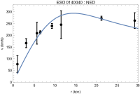
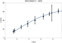
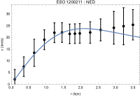
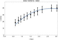
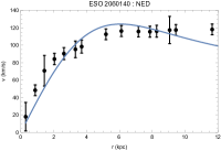
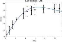
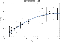
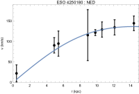
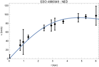
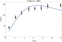
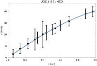
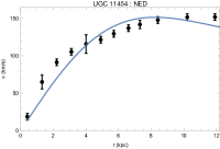
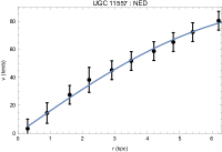
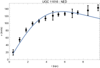
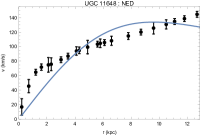
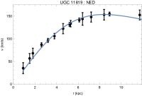
Figure 4: We show, for each one of the galaxies in the sample in Table 2, the plots of the NED theoretical rotation curve (blue solid line), that best fit of the corresponding observational data (black symbols).

Notice how galaxies UGC 11648 and UGC 11748 are the worst fitted cases. This was also the case in Ref. de Blok et al. (2001) for PISO and NFW models. For NED $\chi^{2}_{\rm red}=11.531$ and $16.596$, respectively. Also notice that we have found a preferred range of $\sqrt{\theta}$ values, from $0.5$ to $4.8\;\rm kpc$, approximately.

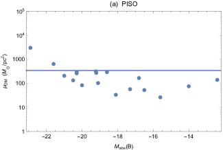
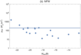
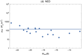
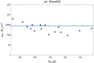
Figure 5: Plots of $\mu_{DM}$ versus the absolute magnitude in the B-band of each galaxy (column (5), Table 2). In (a) is the PISO model; (b) NFW model; (c) Burkert model;(d) NED model and (e) WaveDM model. The mean value of $\mu_{DM}$ is shown to guide the eye (solid line) in each plot.

In Ref. Kormendy and Freeman (2004) was found for PISO model that the surface density $\mu_{DM}$ has nearly a constant value of the order of 100 $M_{\odot}/$pc². This work was extended to include more galaxies and other cored DM models in Spano et al. (2008); Donato et al. (2009). Authors found that its value is almost constant for galaxies in a width range of magnitude values. This indicates that $\mu_{DM}$ should be a quantity characterizing dark matter in galaxies. Following the results in Ref. McGaugh et al. (2016) that used the newly SPARC galaxy catalog, a theoretical study was done in Ref. Ureña-López et al. (2017). We redo these theoretical estimations to find the theoretical values for the DM models we are interested in: PISO, NFW, Burkert, NED and WaveDM. There were differences among PISO and Burkert values we have obtained with the values reported in Ref. Ureña-López et al. (2017). In Tables 3 for PISO model, 4 for NFW model, 5 for Burkert model, 6 for NED model and 7 for WaveDM model, we reported this surface density values, column (4) in each table. In Fig. 5 we have plotted $\mu_{DM}$ versus $M_{\text{abs}}(B)$ for all models.

For PISO model the mean value of $\mu_{DM}$ is $341.64\,M_{\odot}/$pc² while the theoretical value we found, following Ureña-López et al. (2017), is $193\,M_{\odot}/$pc². For NFW: $\mu_{DM}$ is $195.59\,M_{\odot}/$pc² versus the theoretical value of $89\,M_{\odot}/$pc². For Burkert: $\mu_{DM}$ is $462.11\,M_{\odot}/$pc² versus the theoretical value of $348.69\,M_{\odot}/$pc². For NED DM model we have that the mean value of $\mu_{DM}$ is $144.21\,M_{\odot}/$pc² versus its theoretical value of $\mu_{DM}$ is $116.97\,M_{\odot}/$pc². And for WaveDM model we obtained that the mean value of $\mu_{DM}$ is $797.59\,M_{\odot}/$pc² while the theoretical value is $648.58\,M_{\odot}/$pc². This work should be extended to consider more galaxies in order to test more throughly the theoretical predictions as it was done in Ref. Donato et al. (2009).

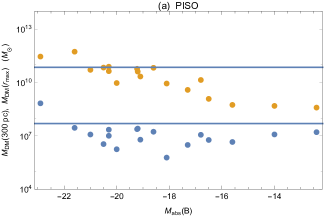
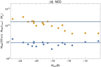
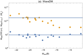
Figure 6: Plots of the $M_{DM}$ versus the absolute magnitude in the B-band of each galaxy (column (5), Table 2). In (a) is the PISO model; (b) NFW model; (c) Burkert model; (d) NED model and (e) WaveDM model. The mean value of $M_{DM}(300$ pc$)$ and $M_{DM}(r_{\text{max}})$ is shown to guide the eye (solid line).

In column (5) of each one of the Tables 3, 4, 5 and 6, we have reported values of the masses of the DM models up to $300$ pc, $M_{DM}(300$ pc$)$, and they were plotted versus $M_{\text{abs}}(B)$ (lower filled circles) for all models in Fig. 6. To guide the eye we have plotted the mean values of $M_{DM}(300$ pc$)$. The mean values we found for each one of the models are: PISO: $4.85\times 10^{7}\,M_{\odot}$; NFW: $1.03\times 10^{8}\,M_{\odot}$; Burkert: $1.79\times 10^{7}\,M_{\odot}$; NED: $0.79\times 10^{7}\,M_{\odot}$; WaveDM: $0.85\times 10^{7}\,M_{\odot}$. In Ref. Strigari et al. (2008) was reported this mass within the central $300$ pc for 18 dSph Milky Way satellites. The value found is about $10^{7}\,M_{\odot}$ which is consistent with the mean values we found except for NFW DM model whose value is an order of magnitude larger. This would indicate that NFW is a model that can not explain rotation curves in spiral galaxies.

Also, in Tables 3, 4, 5, 6 and 7, column (6), we reported values for the total mass of the DM models up to the last spatial point measured, $r_{\text{max}}$. This mass, $M_{DM}(r_{\text{max}})$, was plotted in Fig. 6 (upper filled circles). Values of this total mass fail to follow the constant mean value, almost of the order of $10^{10}\,M_{\odot}$ for all models. In the case of NED, this is in tension with the result reported in Ref. Hernandez-Almada and Garcia-Aspeitia (2016). But we believe more work is needed in order to make a final conclusion.

Finally, for NED model, Fig. 7 shows in (a) the fitted values of parameters $\sqrt{\theta}$ versus $\rho_{NED}$ that include the error bars. In (b) it is shown contour plots for each galaxy at $1\sigma$ and $2\sigma$. This latter plot shows that $\sqrt{\theta}$ and $\rho_{NED}$ are anti-correlated as is always the case for this kind of rotation curve models described by two parameters in a general form similar to Eq. (17).

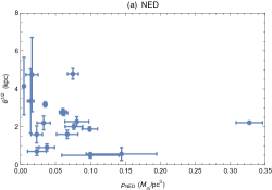
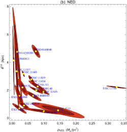
Figure 7: (a) Plots of $\sqrt{\theta}$ versus $\rho_{NED}$ for the NED model, errors bars are also shown. In (b) is the plot of contours at $1\sigma$ and $2\sigma$ of the estimated parameters for each one of the rotation curves of the galaxies studied in this work.

IV Discussion and conclusions

In this paper we have assumed that NED is an important component in Universe dynamics affecting the stellar equations of motion and the dynamic of galaxies in special the rotation curves. From here, it is possible to discuss the research shown in this paper in two main cases:

In the first case, we use the dynamic equations for the evolution of stars with the aim of investigate the behavior dictated by the presence of an uniform density (incompressible fluid) and NED. We find a constraint for the parameter $\sqrt{\theta}$ under the premise of observing important effects in the dynamics of effective pressure and mass, always comparing with the traditional knowledge of the uniform density stars. In this vein, we give to the task of constraint the NED parameter as: $\sqrt{\theta}<0.753R$, emphasizing how the effects induced by NED, generates a not expected behavior.

In addition, with polytropic stars it is possible to model Dwarf Stars with index $n=3$. Here we also add NED which does not interact with the polytropic fluid, presenting a modified Lane-Emden equation to describe the dynamics of the star, our results present important effects in the dynamics except for values that fulfill the conditions $\kappa\geqslant 10^{2}\sqrt{\theta}$ and $\kappa\leqslant\sqrt{\theta}$. We establish our bounds, with a plot in which the correction is negligible, that is, when $\bar{\theta}\to 0$, hence, we can infer those that are mimicked with the traditional limit.

The second case took into account the corresponding rotation velocity of galaxies, assuming that NED is related with the galaxy halo. From here, we compute the rotation velocity associated with this model and was compared with four of the most studied and accepted models in literature, which are: PISO, NFW, Burkert and WaveDM. The analysis was implemented through a $\chi^{2}$ best fit, with eighteen high resolution rotation curves of LSB galaxies with no photometry. The range of values predicted by the method was from $\simeq 0.5$ kpc to $\simeq 5$ kpc. Also, the $\chi^{2}$ best fit for NED was not the most accurate in comparison with the other standard models (see Tables 3, 4 and 5); however it is important to remark that although it was not the best fitting model, the advantage lies in the comparison with NC which is inspired by the internal property of the space-time and not relinquish to this characteristics.

For each DM model and for each galaxy in the analyzed sample we computed three important quantities that should give us information about galaxy formation and evolution that are summarized in Table 8: the surface density $\mu_{DM}$ and the masses within the 300 pc, $M_{DM}(300$ pc$)$, and $M_{DM}(r_{\text{max}})$ for the DM haloes. From other studies it was expected that these quantities were nearly constants, independent of the absolute magnitude of the galaxiesKormendy and Freeman (2004); Ureña-López et al. (2017); Strigari et al. (2008); Hernandez-Almada and Garcia-Aspeitia (2016). The general tendency, found in this work, is that these quantities are roughly constant (except the behavior of $M_{DM}(r_{\text{max}})$). We found like in Strigari et al. (2008), for dwarf spheroidal galaxies, that also must be a common mass for spiral galaxies within $300$ pc and with the same order of magnitud, $10^{7}$ $M_{\odot}$. This would give a central density for DM of $\sim 0.1M_{\odot}$pc^-3, independent of the DM model with the exception of NFW model whose value is an order of magnitud larger. If this result is confirmed NFW would have problems to explain the observed rotation curves of spiral galaxies. The theoretical and observational predictions give that the surface density, $\mu_{DM}$, is constant, independent of the absolute magnitud of the galaxy, but it depends on the DM model. We also found a roughly constant behavior in the surface density in each one of the analyzed models. On the other hand the total mass up to the outer spatial point, $r_{\text{max}}$ fail to have this behavior, this is in tension with a previous result found in Ref. Hernandez-Almada and Garcia-Aspeitia (2016). However, we believe that it is needed a more systematic study with a better sample of galaxies to reach a final conclusion.

Our results about NED parameter are summarized in Table 9 showing the difference between each constraint. It is possible to observe that stellar dynamics provides a lower bound for the free parameter meanwhile galaxy rotation curves provides a higher bounds: an interval of values for the NED parameter. Nevertheless, the rotation curves analysis is less restrictive unlike the toy model cases of stellar analysis; presenting the first one a better confidence in the value. We emphasize that it is necessary to perform a further analysis in both cases to uncover and narrow the free parameter for this matter inspired by NED models. Each model provide us with different results, which are subjected to the astrophysical system to which it is being addressed. However, it is possible to establish a range of values where the NED parameter must fit in.

Results Compilation for $\mu_{DM}$ and $M_{DM}(300$ pc$)$
	PISO	NFW	Burkert	NED	WaveDM
$\hat{r}$	1.52	0	0.96	1.94	0.36
$\hat{g}_{\text{max}}$	2.89	$2\pi$	1.60	4.77	0.86
$\langle\mu_{DM}\rangle$	341.64	195.59	462.11	144.21	797.59
$\mu_{DM}$	193.00	88.73	348.69	116.97	648.58
$\langle M_{DM}(300$ pc$)\rangle$	$4.85$	$10.3$	$1.79$	$0.79$	0.85

Table 8: Compilation of the results for $\mu_{DM}$ and $M_{DM}(300$ pc$)$ shown through the paper. Here $\hat{r}=r/r_{i}$, where the theoretical maximum is found for the dimensionless acceleration $\hat{g}$ Ureña-López et al. (2017), $r_{i}$ is the scale length for each model, and $\langle\mu_{DM}\rangle$ and $\langle M_{DM}(300$ pc$)\rangle$ are the mean value of $\mu_{DM}$ and $M_{DM}(300$ pc$)$, respectively, we found for each galaxy in the analyzed sample. $\langle\mu_{DM}\rangle$ and $\mu_{DM}$ are in $M_{\odot}$/pc² and $M_{DM}(300$ pc$)$ is in $10^{7}M_{\odot}$.

Results Compilation
Star with uniform density	Star with polytropic fluid	Galaxy rotation curves
$\sqrt{\theta}<\frac{1}{2}\sqrt{\frac{R}{GM}}R$	$\kappa\geqslant 10^{2}\sqrt{\theta}\;\;\rm and\;\;\kappa\leqslant\sqrt{\theta}$	$0.5$ kpc $<\sqrt{\theta}<5$ kpc

Table 9: Compilation of the results shown through the paper for the constriction of NED parameter.

The results provided by this paper, contributes to generate astrophysical bounds of the $\theta$ parameter which was studied previously in Ref. Rahaman et al. (2012), but leaving aside the contrast with real data. Of course, we remark that our results are not about NC, instead is just a model that was motivated by NC. NC it is a quantum-gravity theory which has not important effects at macroscopic scales.

As a final note, we remark that the density profile inspired by NC can be used in cosmological analysis like structure formation, the statistics of the distribution of galaxy clusters, the temperature anisotropies of the cosmic microwave background radiation (CMB) and with other astrophysical studies. However, this work is in progress and will be reported elsewhere.

Appendix A PISO, NFW, Burkert and NED Rotation Curves

Here we give a brief summary of three important models found in the literature Begeman et al. (1991); Navarro et al. (1997); Burkert (1995) and the NED rotation curve model. In general, given a dark matter model with a mass profile, $M_{DM}(r)$, a rotation curve is described by (15) written in the following form

$$V_{\rm DM}^{2}(r)=\frac{GM_{\rm DM}(r)}{r},$$ (19)

where the mass at a given radius $r$ is given by

$$M_{\rm DM}(r)=4\pi\int_{0}^{r}dr^{\prime}r^{\prime 2}\rho_{DM}(r^{\prime}/r_{c}).$$ (20)

The function $\rho_{DM}(r/r_{c})$ is a function of $r/r_{c}$ multiplied by $\rho_{c}$. Parameters $\rho_{c}$ and $r_{c}$ characterize the DM density profile. The density at the core of the halo is $\rho_{c}$ and $r_{c}$ is its scale length. It have turned out that the quantity

$$\mu_{DM}(r)=\rho_{c}\,r_{c}$$ (21)

is almost a constant when we fit to observations.

1. Pseudo isothermal profile. Here we consider that DM density profile is given by PISO Begeman et al. (1991) written as:

   $$\rho_{\rm PISO}(r)=\frac{\rho_{p}}{1+(r/r_{p})^{2}}.$$ (22)

   With this density profile it is possible to obtain the mass at a given radius $r$

   $$M_{\rm PISO}(r)=4\pi r_{p}^{3}\rho_{p}\left(\frac{r}{r_{p}}-\arctan\left(\frac{r}{r_{p}}\right)\right),$$ (23)

   and from (19) together with (23) we have

   $$V_{\rm PISO}^{2}(r)=\frac{GM_{\rm PISO}(r)}{r},$$ (24)

   known as PISO rotation velocity Begeman et al. (1991).

2. Navarro-Frenk-White profile. Another interesting case (motivated by cosmological $N$-body simulations) is the NFW density profile Navarro et al. (1997), which is given by Navarro et al. (1997):

   $$\rho_{\rm NFW}(r)=\frac{\rho_{n}}{(r/r_{n})(1+r/r_{n})^{2}}.$$ (25)

   From (20) with the above density profile we have

   $$M_{\rm NFW}(r)=4\pi r_{n}^{3}\rho_{n}\left(\ln(1+r/r_{n})-\frac{r/r_{n}}{1+r/r_{n}}\right).$$ (26)

   From (19), together with (26) we obtain the following rotation velocity:

   $$V_{\rm NFW}^{2}(r)=\frac{GM_{\rm NFW}(r)}{r},$$ (27)

   this equation is known as NFW rotation velocity.

3. Burkert profile. Another density profile proposed by Burkert Burkert (1995) is:

   $$\rho_{\rm Burk}=\frac{\rho_{b}}{(1+r/r_{b})(1+(r/r_{b})^{2})}.$$ (28)

   Again from (20) with the above density profile we have

   $$M_{\rm Burk}(r) = 4\pi r_{b}^{3}\rho_{b}\frac{1}{4}\left(\ln\left[(1+r/r_{b})^{2}(1+(r/r_{b})^{2})\right]\right.$$ (29)

   $$\left.-2\tan^{-1}(r/r_{b})\right).$$

   Again, from (19), together with (28) we obtain the following rotation velocity:

   $$V_{\rm Burk}^{2}(r)=\frac{GM_{\rm Burk}(r)}{r},$$ (30)

   which is known as Burkert rotation velocity Burkert (1995).

4. NED profile.

   Here we consider that DM density profile is given by NED density profile:

   $$\rho_{\rm NED}(r)=\rho_{NED}\exp(-r^{2}/4r^{2}_{NED}),$$ (31)

   where $r_{NED}=\sqrt{\theta}$. As before with this density profile it is possible to obtain the mass at a given radius $r$

   $$M_{\rm NED}(r) = 4\pi r_{NED}^{3}\,\rho_{NED}2\left[\sqrt{\pi}\,\text{erf}(r/2r_{NED})\right.$$ (32)

   $$\left.-(r/r_{NED})\exp(-r^{2}/4r_{NED}^{2})\right],$$

   and from (19) together with (32) we have

   $$V_{\rm NED}^{2}(r)=\frac{GM_{\rm NED}(r)}{r},$$ (33)

   known as NED rotation velocity.

5. WaveDM profile.

   Here we consider that DM density profile is given by WaveDM density profileBernal et al. (2017):

   $$\rho_{\rm WDM}(r)=\frac{\rho_{w}}{(1+(r/r_{w})^{2})^{8}}.$$ (34)

   As before with this density profile it is possible to obtain the mass at a given radius $r$

   $$M_{\rm WDM}(r) = 4\pi r_{w}^{3}\,\rho_{w}\left[\frac{1}{215040\left(\left(\frac{r}{{r_{w}}}\right)^{2}+1\right)^{7}}\right.$$

   $$\times\left(48580\left(\frac{r}{{r_{w}}}\right)^{3}-\frac{3465r}{{r_{w}}}\right.$$

   $$+101376\left(\frac{r}{{r_{w}}}\right)^{7}+92323\left(\frac{r}{{r_{w}}}\right)^{5}$$

   $$+23100\left(\frac{r}{{r_{w}}}\right)^{11}+65373\left(\frac{r}{{r_{w}}}\right)^{9}$$

   $$+3465\left(\frac{r}{r_{w}}\right)^{13}$$

   $$\left.+3465\left(\left(\frac{r}{r_{w}}\right)^{2}+1\right)^{7}\tan^{-1}\left(\frac{r}{r_{w}}\right)\right],$$

   and from (19) together with (LABEL:massWDM) we have

   $$V_{\rm WDM}^{2}(r)=\frac{GM_{\rm WDM}(r)}{r},$$ (36)

   known as WaveDM rotation velocity.