Simple and efficient self-healing strategy for damaged complex networks

Abstract

The process of destroying a complex network through node removal has been the subject of extensive interest and research. Node loss typically leaves the network disintegrated into many small and isolated clusters. Here we show that these clusters typically remain close to each other and we suggest a simple algorithm that is able to reverse the inflicted damage by restoring the network’s functionality. After damage, each node decides independently whether to create a new link depending on the fraction of neighbors it has lost. In addition to relying only on local information, where nodes do not need knowledge of the global network status, we impose the additional constraint that new links should be as short as possible (i.e. that the new edge completes a shortest possible new cycle). We demonstrate that this self-healing method operates very efficiently, both in model and real networks. For example, after removing the most connected airports in USA, the self-healing algorithm re-joined almost 90% of the surviving airports.

I Introduction

A property of critical importance for complex networks is their resilience to damage or attack 1 ; 2 ; 3 ; 4 ; 5 . One fascinating demonstration of the underlying complexity of these systems is that compromise in structure can be substantial even after the loss of a very small number of nodes 6 ; 7 . The repercussions to the network from this structural compromise can be immense, usually resulting in complete loss of communication among the surviving nodes and therefore a complete destruction of the intended network functionality. Because of the obvious importance for practical applications, the robustness of a network’s structure to damage has continuously remained the focus of intensive research in the network science literature 8 ; 8a ; 8b ; 8c ; 8d ; 8e .

Even though we now have a thorough understanding of complex network disintegration, the inverse process of ‘healing’ a network is much less understood. Is there a direct relationship between healing structural features and restoring function? What does it really take for a network to restore its functionality after losing some of its nodes? While there are various types of healing, one realistic approach is to consider the case in which disabled nodes have been permanently removed and cannot be resurrected, but the surviving nodes can still generate new links to other surviving nodes. Of course, a node could trivially create as many new links as possible, but in many realistic settings the cost and time associated with establishing a new link can be high. We then need to optimize the network functionality given the constraints of rebuilding costs Schneider . As a natural first case, we explore the scenario in which optimal network functionality is achieved under the structural condition that all the nodes are connected in one large cluster. In this way, every node can reach any other node in the network, even if the connecting path may be long. This reflects systems such as communication networks 9 ; 10 electrical grids 11 ; 12 , air traffic 13 and shipping routes 14 , etc. Additional requirements can be imposed, for example the maximum path between any two nodes can be bounded 15 , or entirely different cases for structure and function can be explored (e.g. function is optimized when the network structure has a particular degree distribution, or is highly modular, etc.), but as a first approach our only metric here is the size of the largest cluster.

I.1 The Duality of Structure and Function

A basic, but fundamental insight is that healing can be employed with one of two possible goals in mind. The first goal can be to fix the structure in a way that the topology remains as close to the original network as possible. For example, descriptions of some social groups have revealed particular degree distributions and one natural inclination in healing a damaged social network might be to restore edges by focusing on this aspect of repair. However, degree distribution itself is unlikely to support social function. For features such as social identity or support from a close group of friends, the structural features of modularity and clustering are more important. Therefore, if we are attempting repair in order to restore function, we may decide to ignore entirely the impact to degree distribution from repair, instead adding back links that restore (for example) local clustering coefficient. Since damage can alter both structural and functional features, it is easy to consider repairing structure since regaining initial structure should provide restored initial function. Critically, however, it may not be that one and only one structural feature can support the original function. The main question is therefore to discover efficient strategies that can restore network functionality through the addition of new links. In a recent work, redundant (dormant) links were considered to be activated after damage and it was shown that they can restore functionality in infrastructure trees 16 ; 17 . Similarly, healing in interdependent networks was shown to prevent cascading failures 18 . In a different approach, nodes were allowed to spontaneously recover and become active again, leading to an interesting behavior of phase-flipping where the network switches between high-activity and low-activity modes 19 ; 20 . Under different definitions of network function in which a global minimum traffic flow must be maintained and each node has a particular flow capacity that must be redistributed in case of damage, the network functionality can be restored by mitigation strategies 21 ; 22 .

One critical and under-discussed feature of damage, especially in inhomogeneous complex networks, is that the impact from the loss of a single link on overall function can differ drastically depending on where that link occurs in the local and global structure. Loss of a single link that uniquely connects two otherwise disconnected components of a network will have a greater impact to functions (such as the one we study) that rely on the size of the largest cluster than would the loss of one of the three links that make up a triangle. While obvious, it is nevertheless important and profound that we consider healing as a process that should focus on areas of the network in which the most damage has been done to the function, rather than to the structure. In the case of our largest connected component example, this means we should focus more effort towards creating new edges that restore connectivity to nodes that are most direly impacted in their ability to relay messages.

I.2 Local Repair for Global Function

Phrased in this way, it may seem as though the only option is to analyze global network structure in order to understand which nodes are most critical to restoring function. Such a global algorithm could potentially locate the optimal solution by mapping the current state of the network and adding only the links that are missing to restore functionality. However, this centralized planning may not always be feasible, since it may cost a lot in terms of advance planning, communication between the central authority and the individual nodes, the time that it takes to transmit all relevant information, the possibility that communication takes place through the network itself and the central node may have been functionally disconnected from this critical communication, as well as any combination of the above factors which may limit the ability of constructing one central plan and communicate it to all the surviving nodes. Luckily, there is no need for this type of centralized global analysis. We proceed to propose a self-organizing healing algorithm that exploits this heterogeneity feature of damage while relying only on local information accessible to each node, and with low cost from the construction of new links.

Since one of our goals will be to limit the amount of centralized information that will be necessary before repair to the network can begin, we propose purely local definitions of damage that can be assessed by each node. To make this distinction clearly, in this work optimal ‘healing’ will refer to adding new links so that every node can reach any other node in the system, and the term ‘self-healing’ indicates that individual nodes decide on their own whether they need to create new links or not.

I.3 Self-Healing Algorithm to Restore Function

We here demonstrate that our self-healing model can restore connectivity function very efficiently in two different ways. Firstly, we show effective restoration of function with the creation of very few new links relative to the number lost to damage. We demonstrate the effectiveness of the method through the size of the healed largest component, the number of nodes that need to form new links, and the changes in modularity compared to the original network. We further show this is true even if we impose cost constraints on the length of new links (i.e. the number of links in the shortest path required to connect the two nodes without the addition of the new link). Secondly, we show that a null healing model (in which the same number of links are constructed randomly) achieves a drastically lesser restoration of function. We analyze the efficiency of our self-healing algorithm over various network topologies and in cases of both random-node-removal damage and when damage is targeted to affect only specific, high-structural-impact nodes. Based on this ‘uneven damage to function’ perspective, we show that relatively inexpensive, rapid healing may be relatively easy to achieve, even in the absence of global information.

To formalize the problem, we consider the simplest possible case of an isolated complex network which undergoes a loss of a fraction of its nodes, resulting in a possible loss of large-scale connectivity. To mitigate this loss of function, each node can then generate one new link in an attempt to restore connectivity. As mentioned above, this is a trivial problem without any additional constraints because connecting to random nodes would result in a structure similar to an Erdos-Renyi network. In our work, we study what conditions are necessary and sufficient to restore connectivity under the constraints that: a) establishing a new link is costly and that cost is borne by the node initiating the link, b) the new links are as short as possible (based on the path distances of the undamaged network), and c) the decision is purely local, so that a node does not know anything about the network state, except for its own neighborhood. We show that these conditions can be easily met through a simple local-decision algorithm, based on the number of surviving neighbors. There is no need to transfer any information between nodes, and the only requirement is that a node can know if a neighbor within a given distance remains alive or not.

II Results

II.1 Impact of node removal

The first step in identifying efficient healing algorithms is to determine the state of the network immediately after the removal process. This topic has not received attention in the existing literature, which instead mainly focuses only on the properties of the largest connected cluster. For the purpose of a healing algorithm, we consider all the clusters that remain in the system after a fraction $p$ of system nodes have been removed. A possible measure that can quantify the extent of damage is the minimum distance between these clusters, $r_{\rm sep}$, which we define as the minimum possible distance from a node in the cluster to any other node in any other cluster. Since all clusters are disconnected, this distance is calculated in terms of the original network. In practice, we renormalize the damaged structure in the following way (Fig. 1A-D): Every cluster is substituted by one super-node. All these super-nodes are obviously isolated. We restore all the removed nodes and links among them. The links that were connecting removed nodes with any node contributing to a super-node result in a link between the super-node and the removed node (we also remove any double links). In this renormalized network, we can then calculate how close the super-nodes are to each other. Obviously, this distance is bounded by the minimum value of $r_{\rm sep}=2$. Notice also that this distance is different from the distance between a random node in the cluster and other clusters, since it is solely determined by the one node in the cluster which is closest to another cluster.

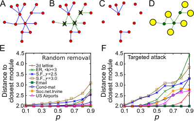
Figure 1: (Color online) Cluster distance after damage. (A) A toy network. (B) A number of nodes are removed from the network. (C) The remaining clusters in the network. (D) We consider each cluster to be one unit. The distance between the clusters, $r_{\rm sep}$, is measured according to the distances of cluster nodes in the original network. (E) The change of inter-cluster distance, $r_{\rm sep}$, as a function of removed nodes, $p$, for model and real networks after random node removal. (F) The change of inter-cluster distance, $r_{\rm sep}$, as a function of removed nodes, $p$, for model and real networks after targeted node removal.

Intuitively, the inter-cluster distance is small in centralized networks and is large in sparse, extended networks. For example, in a star network where all nodes are connected to a central node, the distance $r_{\rm sep}$ can never be larger than 2 independent of how many nodes we remove. In a one-dimensional lattice this distance can become very large, especially when $p$ becomes large and the gap among surviving clusters increases rapidly. Our focus on inter-cluster distance is to enable estimation of the most efficient length for the healing links. If, for example, typical inter-cluster distances were $r_{\rm sep}=5$ then it would be pointless to add links much shorter than that. Similarly, since one of our goals is to minimize the cost, calculating $r_{\rm sep}$ allows us to avoid constructing unnecessarily long links.

We studied the two typical cases of node removal in complex networks: random removal and targeted attack. In Fig. 1E we show the average $\langle r_{\rm sep}\rangle$ over all clusters as a function of the fraction of randomly removed nodes, $p$. In model networks, such as the two-dimensional square lattice, Erdos-Renyi, and scale-free networks, the value of $\rangle r_{\rm sep}\langle$ remains close to 2 until roughly $p=0.5$. When we remove a larger percentage of the nodes the inter-cluster distance increases up to $\langle r_{\rm sep}\rangle\sim 2.5-3$. In real networks, on the other hand, the average distance never increases significantly, independently of the value of $p$.

In targeted attacks we remove the nodes in decreasing order of their degree. As expected, the targeted attack leads to increasing damage and consequently the inter-cluster distance increases in most of the networks (Fig. 1F), with the exceptions of the email network and the square lattice. The email network includes many strong hubs and, as a consequence, node distances are very short, which also reflects on the inter-cluster distances. For lattices, a targeted attack is the same as random removal, because the degree distribution is a delta function. Since ER networks also have a narrow degree distribution, one might expect that the inter-cluster distance in ER networks would also be independent of the attack strategy. In Fig. 1, we find that the opposite is true. The average distance $\langle r_{\rm sep}\rangle$ increases rapidly after $p=0.5$, and at $p=0.9$ it reaches the highest value we observed, $\langle r_{\rm sep}\rangle\sim 4.5$. This is a result of the absence of hubs. When the majority of the highest-connected nodes have been removed, the small remaining clusters consist only of low degree nodes, which have a low probability of being close to each other since there are no hubs to centralize the network.

So, in general, we observe that the isolated clusters are relatively close to each other, and the inter-cluster distances remain for the largest part close to the minimum value of $\langle r_{\rm sep}\rangle=2$, at least for random removals, while in very few cases does it reach $\langle r_{\rm sep}\rangle=3$ or more under targeted attacks.

II.2 Description of the method

The basic idea of the self-healing method is that each node monitors the fraction, $q$, of its neighbors that remain alive. If this fraction falls below a given threshold $q_{c}$, e.g. $q_{c}$=50%, then the neighbor attempts to establish a new link. This link can be at a maximum distance of $r_{\rm max}$, where distances are always measured as path length in the original network. If there is no node within this distance, then the node abandons its attempt to build a new connection. Importantly, in agreement with the above findings on inter-cluster distance, we show that even if the maximum distance is the smallest possible, i.e. $r_{\rm max}$=2, large-scale connectivity is still restored even though the node has no information about whether or not the new link will connect to the largest cluster, or even if it will connect to a different cluster than the one it currently belongs to.

This process can be dynamic, so that nodes do not even need to be aware that there is an attack, as long as they can monitor how many of their links lead to live nodes, in which case they can respond immediately and attempt to create a new link. This real-time healing is more effective than if the nodes can only attempt to heal once an attack is completed (e.g. surprise attacks, or cases in which new link construction is risky until an attack has concluded) and obviates the need for rigorous definitions of global attacks vs local damage. Here, we show that the self-healing algorithm is efficient, even in this worst-case scenario, where the nodes do not have the capacity to respond until the attack is over.

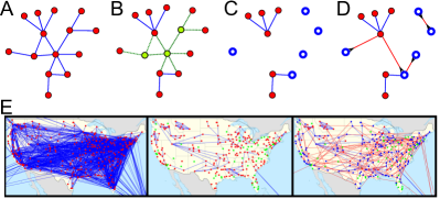
Figure 2: (Color online) Demonstration of the self-healing algorithm. (A) The initial structure of a toy network. (B) Three nodes, indicated by green (light gray), are removed from the network along with all their links. (C) The nodes which have lost half or more of their neighbors (blue nodes, empty symbols) will seek new connections. (D) These nodes will choose to connect to a random surviving node, if its distance $r$ in the original A network is at most $r_{\rm max}$. Here we use $r_{\rm max}=2$. (E) (Left panel) Network of airport connections in USA. (Middle panel) A targeted attack removes the 20% most connected airport nodes, and results to a disconnected network. The removed nodes are shown in green (light gray). (Right panel) The nodes that have lost more than 50% of their neighbors (shown in blue, dark gray) try to establish new links within distance $r_{\rm max}=2$. The new links (red lines) restore the large-scale network connectivity.

The order parameter, which quantifies the large-scale connectivity, is the fraction of the live nodes that belong in the largest connected component, denoted by $P_{1}(p)$ after the attack, and by $P_{2}(p)$ after the healing process. The implementation of this model includes three steps (Fig. 2A-D), which are as follows:

1. A fraction $p$ of the $N$ nodes initially in the system is removed from the network. The size of the remaining largest connected cluster, $P_{1}(p)$, is expressed as a fraction of the remaining nodes.

2. Each of the remaining nodes decides independently if it needs a new link, depending on whether the fraction of its remaining neighbors $q=k_{\rm dam}/k_{\rm orig}$ exceeds a given threshold $q_{c}$ (for any given node, $k_{\rm dam}$ is the number of neighbors after damage, and $k_{\rm orig}$ is the original number of neighbors of this node). We denote the fraction of the surviving nodes that need healing, i.e. those whose degree has fallen below the threshold, as $f$.

3. These $fN(1-p)$ nodes attempt to find a new neighbor within a distance $r_{\rm max}$. If such a neighbor is found, the nodes establish the new link. The fraction of nodes that succeed to establish a new link is $f_{s}\leq f$. These new links then result to a new large cluster that includes a fraction of $P2(p,q_{c})$ [$\geq P_{1}(p)$] nodes.

The size of the largest cluster, $P_{1}(p)$, indicates the extent of damage to the structure immediately after the nodes removal. A value close to $P_{1}(p)=0$ means that the remaining nodes are isolated in small clusters and they cannot access each other. The plot of $P_{1}(p)$ as a function of $p$ represents the well-studied percolation process of the largest cluster as we increase the number of removed nodes. The plot of $P_{2}(p,q_{c})$ can be used to estimate the efficiency of the healing process. After the self-healing process, the largest cluster becomes $P_{2}(p,q_{c})\geq P_{1}(p)$, since we have added links in the structure. The difference between the two sizes is a measure of the process success.

II.3 Self-Healing of the Airport Network

As a real-world example, we can demonstrate how the airport network in USA can be influenced by attacks and healing (Fig. 2E). The unperturbed network (left panel) is quite dense and contains a large number of connections, condensed in many hub nodes. After an intentional attack on 20% of the most connected nodes (middle panel), 80% of the nodes are still functional but are barely connected to other nodes, since most of the traffic was directed through the hubs. The original network contains 332 nodes, so after the removal of 66 nodes we are left with 266 nodes. The largest cluster size connects only 30 of these nodes ($P_{1}\sim 15\%$), and the surviving nodes are either completely isolated or belong to very small clusters. After we apply the self-healing algorithm (right panel), the connectivity is restored and the largest cluster grows to 235 nodes ($P_{2}\sim 88\%$). Of course, the network becomes less centralized as hubs are removed and local connections are added during healing, so that the network topology changes, but the important part is that the functionality is restored and the network becomes navigable again. Now, it is possible to reach practically any node, independently of the origin. In this example it is also easy to see that the new connections have to remain close to the healing node, since the cost of long-range connections may be prohibitively high.

II.4 Self-Healing in Model Networks

The most interesting cases are those where the damage destroys the large-scale connectivity (i.e. $P_{1}(p)$ tends to 0). The question now becomes how easy it is to bring $P_{2}(p,q_{c})$ as close to 1 as possible. Therefore, the main quantities to compare are the values of $P_{2}$ vs $P_{1}$. An ideal process would correspond to a plot of values as close to the horizontal $y=1$ line as possible. This means that, independent of the initial damage, the self-healing process guarantees complete connectivity. The worst-case scenario, on the other hand, is a $y=x$ line along the diagonal, indicating that there is no benefit from the self-healing process.

In Fig. 3 we show the evolution of $P_{1}(p)$ and $P_{2}(p)$ as a function of the removed percentage of nodes, p, in a random removal process. The results for lattices, Erdos-Renyi, and scale-free networks are well known and we recover the typical curves for $P_{1}(p)$ 23 . The self-healing process results in significantly larger critical points for lattice and ER networks. This delay indicates that even though a network has been fully disintegrated, our healing algorithm can reconstitute one large cluster of size $P_{2}(p)$ among the surviving nodes. This improvement is obvious even for large threshold values, such as $q_{c}$=0.75, when a node delays adding a new link until it has lost more than 75% of its neighbors. As we relax this threshold to $q_{c}$=0.5 the largest cluster reaches higher values over a wider $p$ interval. Lowering this threshold even more did not produce noticeable improvement. Therefore, in the following analysis we fix this value to $q_{c}$=0.5.

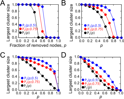
Figure 3: (Color online) Fraction of surviving nodes in the largest cluster as a function of the removed nodes, $p$. The panels correspond to: (A) Two-dimensional square lattice, (B) Erdos-Renyi network with average degree $\langle k\rangle=3$, (C) Random scale-free network with degree exponent $\gamma=2.5$, and (D) Random scale-free network with degree exponent $\gamma=3$. The network size in all cases was $N=10^{5}$ nodes. Black (lower) lines indicate the cluster size $P_{1}(p)$, after the initial removal of nodes. The red (middle) lines represent the cluster size after the healing process, $P_{2}(p;0.75)$, where a node decides to search for new connections if it has lost at least $q_{c}=75\%$ of its original neighbors. The blue (upper) line shows the healed cluster size, $P_{2}(p;0.5)$, for a corresponding threshold of $q_{c}=50\%$. The healing distance in all cases is $r_{\rm max}=2$.

Each node seeks new connections within a maximum distance $r_{\rm max}$, and for the results seen in Fig. 3 we used the minimum possible distance, i.e. $r_{\rm max}$=2. As we increase the radius of possible new connections the connectivity becomes easier to achieve for a number of reasons. First, there are more options because the node can create a link, even if all second-neighbors have been removed. Second, the effect of long-range shortcuts is known to favor large-scale connectivity 24 . For example, if the attack results in small, isolated clusters, then short-range shortcuts will tend to remain within the same cluster and cannot assist in bridging between different clusters. On the other hand, long-range shortcuts will have a much higher probability of bridging otherwise unconnected parts of the network because they can choose nodes that are far from the immediate neighborhood of their initiator 25 . The problem with this approach, of course, is that the associated cost of long links may become significantly higher. It is important, therefore, to know if the minimum possible cost is enough to restore the network structure.

II.5 Efficient Cost-Constrained Repair

As we will demonstrate below, in the absence of cost restrictions, higher values of $r_{\rm max}$ improve the repair results, with the optimum case being that $r_{\rm max}$ is unrestricted and the node can randomly choose any other surviving node in the system. This is a trivial theoretical result, because long-range links can connect isolated clusters which are far from each other in case of extended damage. Importantly, however, beyond this trivial result, we show that the minimum value of $r_{\rm max}$=2 is already sufficient to restore network structure. We therefore focus our discussion by reporting only results for this worst-case scenario.

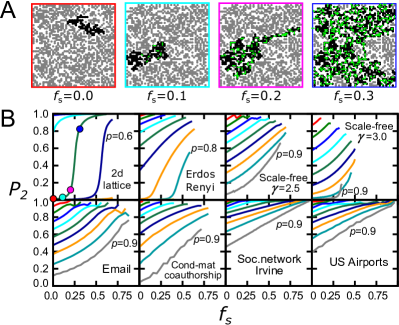
Figure 4: (Color online) (A) Snapshots of the healing process in a square two-dimensional lattice, after removing $p=50\%$ of the nodes. The nodes that survived the attack are shown in gray color, with black nodes indicating the largest cluster after a fraction, $f_{s}$, of the surviving nodes have generated a new link. The healing links are shown in green (light gray on black nodes). (B) Evolution of the largest cluster size during healing, as a function of the percentage of surviving nodes, $f_{s}$, that establish a new link. From top to bottom, the fraction of removed nodes increases in steps of 0.1, from $p=0.1$ to $p=0.9$ (or to the value indicated on the plot). The starting point of each curve at $f_{s}=0$ corresponds to the largest cluster size immediately after the removal of $p$ nodes. The end point of each curve indicates the final cluster size after the end of the healing process.

In Fig. 4 we present many examples of the self-healing process, for both model and real-world networks. A lattice structure offers the simplest example of self-healing. In Fig. 4A we present a toy example, in a lattice where $p=50\%$ of the nodes have been removed. As we add the links to a fraction fs of the nodes that have lost more than half of their neighbors, the size of the largest cluster increases and presents essentially a typical second order percolation transition. This behavior is verified in the first panel of Fig. 4B, where the large-scale connectivity is easily restored for values of $p\leq 0.6$. The second-order transition is observed in all the model networks, but only when the values of $p$ reach close to their critical values pc. For $p<p_{c}$, the initial largest cluster at $f_{s}=0$ extends over a non-zero fraction of the remaining nodes and, notably, there is no transition in these cases. The linear increase of the largest cluster size indicates that the new links attach small clusters to the spanning cluster, and there is never any other cluster of significant size. The absence of a transition is observed in all real networks, even when the initial largest cluster is very small. For instance, at $p=0.9$, the largest cluster size of the co-authorship network starts at less than $P_{1}=5\%$ and with healing it increases almost linearly up to $P_{2}~{}70\%$. Notice that in these plots the process does not necessarily go up to $f_{s}=1$, since not all nodes need, or can find, new connections according to the rules of the algorithm.

We then compare the value of the cluster size at the end of healing, $P_{2}$, with the cluster size before healing, $P_{1}$, for different values of $p$ (Fig. 5). In lattices, we know that close to the threshold $p\sim 0.5$ the system is in the critical phase so that a small number of links are enough to restore connectivity. However, in the plot we can see the large improvement that healing brings to the tolerance of the system. Even though the network disintegrates very rapidly as we remove more nodes and increase $p$ to $p\sim 0.6$, the largest cluster after self-healing practically includes all remaining nodes, so that $P_{2}\sim 0.95$. Moving from $p=0.6$ to $p=0.7$ causes a much greater damage which cannot be restored via our self-healing process and $P_{2}$ abruptly drops to $P_{2}\sim 0$. In practice, the self-healing algorithm has managed to delay the location of the critical point from $p\sim 0.5$ to $p\sim 0.7$. This simple behavior of either a fully connected or fully disconnected cluster is rather idiosyncratic of the highly organized configuration of nodes in the lattice, which is not found in random models and real-world networks, as we show below.

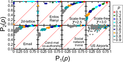
Figure 5: (Color online) How the largest cluster size changes after healing, $P_{2}(p)$, as a function of the largest cluster size before healing, $P_{1}(p)$. Results are presented for model and real-world networks. The percentage of nodes removed is represented by the color of a node, increasing from right to left from $p=0.1$ to $p=0.9$. Each scattered point corresponds to a different realization of the process in each network. The efficiency of the healing process is demonstrated by the fact that all the points tend to be far from the diagonal, which would indicate no improvement, and remain close to the maximum efficiency value of $P_{2}(p)=1$.

The Erdos-Renyi network (with average degree $\langle k\rangle=3$) follows a similar pattern where removing 70% of the nodes results to isolated clusters, $P_{1}(p)\sim 0$. After healing with our algorithm the largest cluster size encompasses a large part of the remaining nodes, $P_{2}(p)\sim 0.8$. This striking difference indicates that the remaining clusters remain close to criticality and relatively close to each other, since they can be merged when nodes add new local links with $r_{\rm max}$=2. Similar improvement is found for the case of scale-free networks with different degree exponents.

II.6 Model vs Real-World Networks

An important difference between random model networks and real-world networks is usually the level of organization. For instance, typical empirical networks exhibit higher degrees of clustering and modularity, features that are missing in the randomly built networks 26 . Nevertheless, this organization can potentially drastically impact the outcome of the healing process. In the examples that we studied (Fig. 5) we see that self-healing is equally, if not more, efficient in restoring the largest cluster in empirical networks. In certain cases, e.g. the friendship social network in Irvine or the email exchange network, practically all the surviving nodes belong to the same cluster after healing, even though the starting network state is highly disintegrated, i.e. $P_{1}(p)<0.2$. Of particular importance is the result for the network of airport connections, because it is a spatially embedded structure and we can approximate spatial distance with network distance, at least to demonstrate the principle that longer jumps may be very costly to implement. The example highlights the importance of small $r_{\rm max}$ values. If an airport closes down then the traffic needs to be redirected to another airport in the general area, but it is impractical if this distance remains unrestricted. Additionally, in this example connectivity is crucial for the network to be functional (one needs to be able to reach any destination). Under the conditions of our self-healing algorithm, the large-scale connectivity was almost certain in all our simulations, with more than 80% of the nodes belonging in the largest cluster. The large fluctuations, especially in the extreme case where 90% of the nodes have been removed, are the result of the small network size, which includes 332 nodes. This demonstrates that healing may become unpredictable for very small networks, where one or two links may be enough to connect the small number of clusters.

The percentage of nodes that find themselves with fewer neighbors than the threshold increases with the number of nodes that are removed. These nodes do not necessarily manage to find a new neighbor within the distance $r_{\rm max}$=2, either because all these nodes have been removed or because there is already a connection. As we show in Fig. 6, all nodes in lattice and in model random networks manage to find a new neighbor as long as less than 50% of the initial nodes have been removed. As the extent of damage increases, a larger percentage of nodes need new connections, but less than half of those manage to do that. On the contrary, in real networks all nodes manage to find new connections almost independently of the extent of damage in the network.

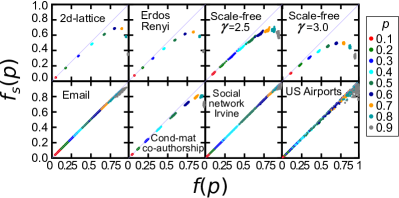
Figure 6: (Color online) Fraction of the surviving nodes that successfully established new connections, $f_{s}$, as a function of the fraction of nodes, $f$, that attempted to establish new connections following the removal of a percentage $p$ of nodes. The value of $p$ increases from left to right. The points that are closer to the diagonal indicate a higher percentage of success.

Even though functionality is restored, since the majority of nodes can now communicate with each other through the structural repair that reconnected a large cluster, it is not clear what impact restoration of this particular structural feature may have on other topological/structural features. We therefore study the effect on the modularity of the healed network compared to the modularity of the undamaged network as an example of a potentially important structural feature which is not necessarily correlated to the size of the largest cluster. We use the standard definition for modularity $Q$, as the fraction of links between modules, minus the expected number of links within these modules for a random graph with the same node degree distribution 26 . For Fig. 6 we report the maximum possible value of $Q$, using the algorithm from Ref. 27 . In Fig. 7 we show changes in modularity after a random removal of $pN$ nodes and the application of the self-healing algorithm. A common trend in both model and real networks is that modularity increases considerably with increasing $p$. This shows that the healing effect tends to create significantly stronger modules, and nodes tend to become more connected within the same network area. Of course, this is the result of the short-range links in the presented simulations, where $r_{\rm max}$=2. In practice, the healing algorithm replaces the links that are removed with local links, enhancing thus the modular character of the network. The only instances where modularity decreases are at large values of $p$ in the model networks. This result can be explained by Fig. 6 where only a small percentage of nodes manage to find new connections and therefore the form of the resulting structure is not very different than the damaged structure.

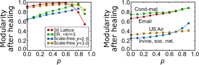
Figure 7: (Color online) Effect of the self-healing process on the network modularity, as a function of the removed nodes. The modularity at $p=0$ corresponds to the original network modularity. For $p>0$, we consider the modularity of the network after healing with $r_{\rm max}=2$.

II.7 Self-Healing vs Random Repair

The efficiency of our method can be tested against a random insertion of links under a similar set of constraints, as for the self-healing algorithm. For example, we can add the same number of links at the same distance, but random nodes are chosen to create new links, rather than those who have lost most of their neighbors. In this way, we can detect if the crucial factor is the number of edges or the particular features of the nodes that select to establish new connections. Even if our model results did not exceed those of random insertion, our method is based on a self-organized algorithm that provides a simple local decision scheme, where there is no need for a central authority to coordinate actions around the network. Still, we demonstrate below that our method, which we tested in a number of model and real-world networks, significantly exceeds the results of random decisions.

We assess the effectiveness of the algorithm by comparing our results to such a null model. In this way, we can determine if there is a benefit to choosing which nodes create new links based on $q_{c}$. For each realization of nodes removal with the self-healing algorithm we calculated how many new links were introduced in the system, resulting to $P_{2}(p)$. We then added the same number of links to the damaged network, but this time the link originated from a random node instead of the node that had lost more than a fraction $q_{c}=50\%$ of its neighbors. These new links were established within a distance $r_{\rm max}$=2, so that the total cost remained the same in both cases. The result in the top row of Fig. 8A shows that the self-healing algorithm performed better in all cases compared to this null model. The reason is that when a random node decides to establish a new link, it is possible that many of its neighbors still survive and the new link does not bring together isolated parts of the network. This is also why when the removed percentage of nodes is small, e.g. 10-20%, there is no increase in the largest cluster size, unless we use the nodes that have lost most of their neighbors.

We also studied the effect of $r_{\rm max}$ on the results (Fig. 8). As expected, we find that as we increase the maximum distance for new connections, the repair process becomes more efficient. As shown in the plot for the self-healing algorithm, $r_{\rm max}=3$ is already enough to completely restore connectivity among all the remaining nodes, practically under any conditions. The optimal case is found for $r_{\rm max}\geq 4$. The results for the random model are consistently inferior to those of our algorithm. The trend of better healing with increasing $r_{\rm max}$ remains, but now even for unrestricted $r_{\rm max}=\infty$, the value of the repaired largest cluster cannot reach the optimal value, $P_{2}(p)=1$.

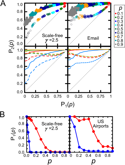
Figure 8: (A) Top row: Comparison of the result for the self-healing algorithm (filled symbols) with adding the same number of links starting from random nodes (empty symbols). In both cases, $r_{\rm max}=2$. Bottom row: Comparison of the self-healing algorithm (continuous lines) with the random case (dashed lines), for different $r_{\rm max}$ values. From bottom to top: $r_{\rm max}$=2, 3, 4, and $\infty$. (B) Comparison of the largest cluster size after an intentional attack.

II.8 Random vs Targeted Attack

Until now, we studied the healing process on networks where the nodes were randomly selected for removal. Another important removal technique simulates intentional attack on the network, where nodes are removed in descending order of their degree, i.e. the highest connected nodes are removed first. This attack requires a much smaller percentage of removed nodes to destroy the network, since all the hubs that glue the network together are removed and the network disintegrates into small pieces. The self-healing algorithm is efficient in this case, too (Fig. 8B). The critical value of $p$ for a scale-free network with degree exponent $\gamma$=2.5 moves from $p\sim 0.05$ to $p\sim 0.5$. This is a huge difference that allows the network to operate even after losing the most connected nodes in its backbone. Similarly, in the case of the airport connection network, the removal of the hubs leads to a disconnected network when 20% of the nodes are removed, but the healed network manages to preserve the largest cluster even if more than 60% of the nodes are removed.

III Discussion

In this paper we make explicit a fundamental feature of damage in complex networks and use it to design a very simple self-healing algorithm to restore connectivity-based function. We show that even just this simple example is enough to restore large-scale connectivity in a severely damaged network, while keeping the reconnection cost low. In this particular scenario of structure enabling function, a node decides based on its own link losses to add a new link to one of its second neighbors (provided at least one survives) without considering any other parameter. This approach has the added benefit that it is strictly local, and every node can make the decision autonomously. The cost is also lower with this strategy compared to selecting random nodes for the same number of links.

The critical insight that working to restore function may not rely on restoring the initial structure allowed us to design a threshold, $q_{c}$. This threshold acts as a natural filter to direct the addition of the links towards the areas where function has been most affected by the damage in this connectivity-based scenario.

In fact, this strategy represents a worse-case scenario, because the nodes make new connections only after the removal of all nodes, or equivalently if the attack takes place faster than the nodes can react. In an alternate version, the algorithm could be applied in a dynamic fashion so that a node continuously monitors its neighbors and decides to add new links based on current information, i.e. as soon as it notices that the number of its neighbors falls below the threshold. Under this scenario, a node could establish more than one new links during the process and it would be easier to preserve long-range connectivity, simply because of the addition of a larger number of links. What we showed above is that this extension is not necessary since a similar result can be achieved with much fewer new connections.

A few interesting parallels can be drawn between the self-healing algorithm and Achlioptas processes 28 . In the latter, we start from an empty network of $N$ nodes which grows by adding new links according to the process rules. These rules can either favor or discourage the emergence of a largest cluster. In our case, the starting point is an already fractioned network, and the goal is to merge all clusters into one giant network with as few links as possible. A key difference is that we only use local decisions, while in typical Achlioptas processes the information of the involved cluster sizes is required.

IV APPENDIX: DATASETS

We analyzed four different networks, based on the following datasets:

1. Email network: Email messages sent at the Computer Sciences Department of London’s Global University http://lisgi1.engr.ccny.cuny.edu/~makse/SOCIAL/Emailcontacts.dat.gz.

2. Cond-mat co-authorship: The network of co-authorship in preprints submitted to the cond-mat section of arxiv.org 29 .

3. Irvine social network: The dataset was downloaded from http://toreopsahl.com/datasets/#online_social_network and has been analyzed in 30 . It includes online messages sent among students at the University of California, Irvine, through a Facebook-like Social Network.

4. USA airport network: A link indicates that two networks are connected by a direct flight. This dataset refers to flights in 1997 and can be downloaded at http://vlado.fmf.uni-lj.si/pub/networks/data/mix/USAir97.net.

References

- (1) R. Cohen, K. Erez, D. ben-Avraham, and S. Havlin, Phys. Rev. Lett. 85, 4626 (2000).
- (2) R. Albert, H. Jeong, and A. L. Barabasi, Nature 406, 378 (2000).
- (3) S. Boccaletti, V. Latora, Y. Moreno, M. Chavez, and D. Hwang, Phys. Rep. 424, 175 (2006).
- (4) D. Helbing, Nature 497, 51 (2013).
- (5) D. J. Watts, Proc. Natl. Acad. Sci. 99, 5766 (2002).
- (6) R. Cohen, K. Erez, D. ben-Avraham, and S. Havlin, Phys. Rev. Lett. 86, 3682 (2001).
- (7) D. S. Callaway, M. E. J. Newman, S. H. Strogatz, and D. J. Watts, Phys. Rev. Lett. 85, 5468 (2000).
- (8) A. A. Moreira, J. S. Andrade Jr., H. J. Herrmann, and J. O. Indekeu, Phys. Rev. Lett. 102, 018701 (2009).
- (9) C. Moore, G. Ghoshal, and M. E. J. Newman, Phys. Rev. E 74, 036121 (2006).
- (10) N. Farid and K. Christensen, New J. Phys. 8, 212 (2006).
- (11) J. Saldana, Phys. Rev. E 75, 027102 (2007).
- (12) C. M. Schneider, L. de Archangelis, and H. J. Herrmann, Europhys. Lett. 95, 16005 (2011).
- (13) H. Bauke, C. Moore, J. B. Rouquier, and D. Sherrington, Eur. J. Phys. B 83, 519 (2011).
- (14) C. M. Schneider, A. A. Moreira, J. S. Andrade Jr., S. Havlin, and H. J. Herrmann, Proc. Natl. Acad. Sci. 108, 3838 (2011).
- (15) M. Faloutsos, P. Faloutsos, and C. Faloutsos, in (ACM, 1999), p. 251.
- (16) J. Onnela, J. Saramaki, J. Hyvonen, G. Szabo, D. Lazer, K. Kaski, J. Kertesz, and A. Barabasi, Proc. Natl. Acad. Sci. 104, 7332 (2007).
- (17) S. H. Strogatz, Nature 410, 268 (2001).
- (18) R. V. Sole, M. Rosas-Casals, B. Corominas-Murtra, and S. Valverde, Phys. Rev. E 77, 026102 (2008).
- (19) B. Monechi, V. D. Servedio, and V. Loreto, PLoS One 10, e0125546 (2015).
- (20) C. Ducruet, C. Rozenblat, and F. Zaidi, J. Transp. Geogr. 18, 508 (2010).
- (21) E. Lopez, R. Parshani, R. Cohen, S. Carmi, and S. Havlin, Phys. Rev. Lett. 99, 188701 (2007).
- (22) W. Quattrociocchi, G. Caldarelli, and A. Scala, PloS One 9, e87986 (2014).
- (23) Y. Shang, Phys. Rev. E 91, 042804 (2015).
- (24) M. Stippinger and J. Kertesz, Physica A 416, 481 (2014).
- (25) A. Majdandzic, B. Podobnik, S. V. Buldyrev, D. Y. Kenett, S. Havlin, and H. E. Stanley, Nature Physics 10, 34 (2014).
- (26) A. Majdandzic, L. A. Braunstein, C. Curme, I. Vodenska, S. Levy-Carciente, H. E. Stanley, and S. Havlin, arXiv preprint arXiv:1502.00244 (2015).
- (27) J. Wang, Physica A 392, 2257 (2013).
- (28) C. Liu, D. Li, E. Zio, and R. Kang, PloS One 9, e112363 (2014).
- (29) M. E. J. Newman, Networks: An Introduction (Oxford University Press, New York, 2010).
- (30) J. M. Kleinberg, Nature 406, 845 (2000).
- (31) H. D. Rozenfeld, C. Song, and H. A. Makse, Phys. Rev. Lett. 104, 025701 (2010).
- (32) M. E. Newman, Proc. Natl. Acad. Sci. 103, 8577 (2006).
- (33) A. Clauset, M. E. J. Newman, and C. Moore, Phys. Rev. E 70, 066111 (2004).
- (34) D. Achlioptas, R. M. D’Souza, and J. Spencer, Science 323, 1453 (2009).
- (35) M. E. J. Newman, Proc. Natl. Acad. Sci. 98, 404 (2001).
- (36) T. Opsahl and P. Panzarasa, Soc. Networks 31, 155 (2009).