Quantum galvanometer by interfacing a vibrating nanowire and cold atoms

Abstract

We evaluate the coupling of a Bose-Einstein condensate of ultracold, paramagnetic atoms to the magnetic field of the current in a mechanically vibrating carbon nanotube within the frame of a full quantum theory. We find that the interaction is strong enough to sense quantum features of the nanowire current noise spectrum by means of hyperfine-state-selective atom counting. Such a non-destructive measurement of the electric current via its magnetic field corresponds to the classical galvanometer scheme, extended to the quantum regime of charge transport. The calculated high sensitivity of the interaction in the nanowire-BEC hybrid systems opens up the possibility of quantum control, which may be further extended to include other relevant degrees of freedom.

Carbon nanotube (CNT) technology has evolved to the point, where CNTs can be produced with a variety of mechanical and electrical properties Harris (2009). Besides applications in chemical Kong et al. (2000), biological Lin et al. (2004a), and mass sensing with up to single atom resolution Chiu et al. (2008), high quality nanomechanical resonators Hüttel et al. (2009), one-dimensional electric transport effects and their coupling to mechanical motion of the CNTs have been observed Steele et al. (2009); Lassagne et al. (2009). The increasingly fine control of these degrees of freedom anticipates the manipulation of CNTs at a quantum mechanical level that has been recently achieved in other nanomechanical systems O’Connell et al. (2010).

Atomic physics has undergone a breathtaking evolution since laser cooling and trapping techniques allowed for the preparation of localized and isolated atom samples Chu et al. (1998). The thermal noise has been reduced to the ultimate quantum noise level where the “ultracold atoms” (below 1$\mu$K) form a degenerate quantum gas, called a Bose-Einstein condensate (BEC) Castin (2001). This cloud of atoms can be controlled in all relevant degrees of freedom with an unprecedented precision. The cloud can be positioned on the submicrometer scale in magnetic Fortágh and Zimmermann (2007) or optical traps Grimm et al. (2000). The internal electron dynamics can be driven by external laser or microwave fields which allow for the precise preparation as well as the high-efficiency detection of the electronic state. The system of trapped neutral atoms in the collective BEC state is an ideal probe of external fields Wildermuth et al. (2005).

The first attempts to make a BEC interact with a CNT have been reported only recently. Atom scattering from the CNT’s van der Waals potential Gierling et al. (2011), and the field ionization due to charged suspended nanotubes have been observedGoodsell et al. (2010). Recent proposals have discussed how to make use of the CNT as a current-carrying thin nanowire to tighten the magnetic trapping potential for cold atoms Petrov et al. (2009) and how to form nanoscale plasmonic atom traps along silver decorated CNTs Murphy and Hau (2009). The integration of carbon nanotubes and atomic Bose-Einstein condensates opens up new avenues towards hybrid systems coupling these objects at a quantum level in a controlled way. One can envisage the coherent interfacing of very different degrees of freedom such as electronic, mechanical, and spin variables. The question is whether there is a suitable interaction between selected degrees of freedom and whether the cross-coupling is strong enough to design useful quantum devices. A variety of novel nanodevices for precision sensing, quantum measurement, and quantum information processing could be developed on the basis of CNT-BEC coupling.

In this Letter we theoretically evaluate the interaction between the current through the nanowire and atoms in a condensate. We describe how the internal atomic dynamics in the hyperfine states couples to the magnetic field generated by the CNT current. Starting from a fully quantum model we calculate the time evolution of the atomic system and construct a scheme to measure the current via an atomic observable. All this leads to the conclusion that quantum dynamical properties of the CNT are detectable by making use of the mature technology of ultracold atoms. A more general implication is that the other degrees of freedom of the CNT and BEC which take part in the dynamics can also be accessed and possibly manipulated in variants of this scheme.

For the sake of concreteness, we focus on the measurement of the current through the CNT in the galvanometer scheme, i.e., when the electric current is sensed in a non-destructive way via its magnetic effect. We are interested in the quantum transport limit of a mesoscopic conductor. In principle, a quantum object such as a spin-1/2 particle precessing in the magnetic field is sensitive to the quantum properties of the current. The full counting statistics of the charge transport process Bednorz and Belzig (2010) can be reconstructed from the density matrix of the spin Levitov (2003). This scheme is sometimes referred to as the quantum galvanometer Levitov et al. (1996). However, its realization has to meet several conditions (stability, sensitivity and detectability, see below), which has seemed out of the question so far.

In our scheme the fictitious spin of the quantum galvanometer is realized by a cloud of long-term trapped atoms. One can make use of the collective BEC state which greatly enhances the sensitivity of the internal hyperfine dynamics to external magnetic fields Vengalattore et al. (2007). Moreover, a direct readout method for the spin state is available since the populations in the magnetic sublevels can be counted by state selective ionization with single-atom resolution Stibor et al. (2010). The populations are expressed in the diagonal elements of the spin density matrix. In principle, the off-diagonal elements could also be measured, which is required to determine the generating function of the full counting statistics. Here we propose a simpler measurement restricted to the diagonal elements, since it is already enough to characterize some of the quantum features of the current. In particular, we will show that the ordinarily defined current noise spectrum,

$$S(\omega)=\int_{-\infty}^{\infty}d\tau e^{i\omega\tau}\left<\hat{I}(0)\hat{I}\left(\tau\right)\right>\,,$$ (1)

is directly related to the time evolution of the populations in the given magnetic sublevels. The proposed galvanometer allows for the measurement of the spectrum by scanning the adjustable variable $\omega$ which spans both the negative and positive frequency ranges. Asymmetry of the measured spectrum around $\omega=0$ would reveal quantum features Nazarov and Blanter (2009). This is due to the fact that asymmetry of $S(\omega)$ is equivalent with the non-commutativity of the current operator at different instances, as one can easily check in the above equation.

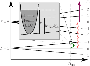
Figure 2: Level scheme of the ⁸⁷Rb atoms. The inset shows the resonance condition for the $m=-1\leftrightarrow 0$ rf transition induced by the time-varying magnetic field component due to the oscillating CNT. The shaded region corresponds to the band of energies in the Thomas-Fermi approximation. The detection of atoms in the spatially separated state $F=1,m=0$ is performed by a resonant microwave excitation to $F=2,m=0$ (curly arrow), and then by a two-photon ionization process Stibor et al. (2010) (double arrow).

The scheme is presented in 1 for a possible architecture of building the galvanometer on an integrated platform, the so-called “atomchip” Fortágh and Zimmermann (2007); Folman et al. (2002). It is a compact, substrate-based electric circuit of currents which create highly tunable magnetic traps for the neutral atoms. The chip may support a contacted CNT on the side facing the BEC. The suspended CNT is a high-Q mechanical oscillator Sazonova et al. (2004); Witkamp et al. (2006); Hüttel et al. (2009); O’Connell et al. (2010), which is driven to oscillate coherently with large amplitude. We note that in order to simplify our calculations, here we assume that the vibration of the CNT is driven by a mechanical source (e.g. a piezo crystal) instead of electric fields. Therefore the CNT current generates a harmonically time-varying magnetic field. In the neighboring BEC, this field may excite transitions between the hyperfine states. The key role of the mechanical vibration of the CNT consists in creating the resonance conditions such that the low-frequency components of the current noise spectrum be close to resonance with the hyperfine transitions (Zeeman splitting), c.f. Fig. 2. Initializing the atoms in the BEC in a well-defined hyperfine state, the number of atoms transferred to another state follows a statistics determined by the low-frequency part of the current noise spectrum. The noise source can be arbitrary, e.g., thermal or intrinsic quantum noise; for generality, we will represent the current as a quantum operator in the derivation. Finally, the measurement is accomplished by detecting the number of transferred atoms in a given time period, which can be performed by means of state-selective ionization technique at the single-atom resolution level Stibor et al. (2010).

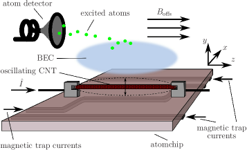
Figure 1: The quantum galvanometer on an atomchip. A BEC is loaded into the magnetic microtrap created by the classical electric currents through integrated conductors on a dielectric substrate Fortágh and Zimmermann (2007) (represented on the bottom of the chip). A suspended carbon nanotube is also part of the electric circuit Petrov et al. (2009) and transports the quantum current. The oscillating CNT creates a magnetic field in the 10 MHz range interacting with the hyperfine transitions of the atoms. Atoms transferred to untrapped states are detected by a single-atom detector Stibor et al. (2010).

To be specific, we consider ultracold ⁸⁷Rb atoms in the hyperfine state $F=1$. The atomic spin $\hat{\mathbf{F}}$ interacts with the magnetic field according to the Zeeman term $H_{Z}=g_{F}\,\mu_{\mathrm{B}}\hat{\mathbf{F}}{\mathbf{B}}({\mathbf{r}})$, where $\mu_{\mathrm{B}}=e\hbar/2m_{e}$ is the Bohr magneton, the Landé factor is $g_{F}=-1/2$, and $\hat{\mathbf{F}}$ is measured in units of $\hbar$. The dominant component of the magnetic field is a homogeneous offset field $B_{\rm offs}$ in the $z$ direction. The eigenstates of the spin component $\hat{F}_{z}$ are then well separated by the Zeeman shift. These are the magnetic sublevels labelled by $m=-1,0,1$. On top of the offset field, there is an inhomogeneous term which creates an ellipsoidal potential around the minimum of the total magnetic field. The atoms are then subject to the static potential $V_{m}({\mathbf{r}})=-mV_{\mathrm{T}}({\mathbf{r}})+g_{F}\mu_{\mathrm{B}}mB_{\mathrm{offs}},$ where $V_{\mathrm{T}}({\mathbf{r}})=\frac{M}{2}\left[\omega_{r}^{2}\left(x^{2}+y^{2}\right)+\omega_{z}^{2}z^{2}\right]$, with $M$ being the atomic mass. The potential is diagonal in the $\hat{F}_{z}$ basis, and is confining only for $m=-1$.

Let us consider a single carbon nanotube of length $L$ which is electronically contacted and carries a current $\hat{I}(t)$. It generates a magnetic field that interacts with the atomic spin. Similar coupling has been considered Treutlein et al. (2007) between a vibrating nanomagnet and a BEC. The CNT is aligned with the $z$ axis (see 1) having a mean distance $y_{0}$ from the condensate. This distance is large enough ($y_{0}\geq 1\mu$m to avoid Van der Waals-type interactions between the atoms and the CNT Fermani et al. (2007); Ristroph et al. (2005); Goodsell et al. (2010); Grüner et al. (2009); Gierling et al. (2011)). The CNT is driven to mechanically oscillate harmonically at an angular frequency $\omega_{\rm cnt}$ in the 10 MHz range Sazonova et al. (2004); Witkamp et al. (2006) and with an amplitude $a$ in the $y-z$ plane ($a\ll y_{0}$). The resulting time-dependent magnetic field $\hat{\mathbf{B}}_{\textrm{cnt}}({\mathbf{r}},t)$ is an operator, since its source is the current operator $\hat{I}$. With a proper tuning of the Zeeman splitting via the offset $B_{\textrm{offs}}$, the $x$ and $y$ components of $\hat{\mathbf{B}}_{\textrm{cnt}}$ can quasi-resonantly generate transitions between the magnetic sublevels $m$. Such a transfer of trapped atoms into untrapped ones is the underlying mechanism of the rf outcoupler of an atom laser Steck et al. (1998). Here a fast detection of the spatially separated component $m=0$ will be required by means of combined microwave transition and two-photon ionization process Stibor et al. (2010) via the state $F=2,m=0$ (see 2).

In the following, we will describe the BEC-CNT interaction based on a model Hamiltonian [2] which treats all the relevant degrees of freedom quantized. Within the Thomas-Fermi approximation (large condensate limit, 3a) and to first order in perturbation theory [4], we will solve the dynamics for the time evolution of the atomic state populations [8]. Thereby, we will obtain a relation between the population in the externally monitored hyperfine state and the current noise spectrum in a closed form [12]. This relation is a convolution which includes a detection spectral function characterizing the resolution of the measurement [11]. We will present its functional form in 3 and discuss how its magnitude depends on the physical parameters of the setup.

The ultracold atom cloud can be described by the spinor fieldHo (1998) $\sum_{m}\hat{\Psi}_{m}\left|F=1,m\right\rangle$. The very general many-body Hamiltonian is given by

$$\!{\mathcal{H}}=\!\int\!d^{3}{\mathbf{r}}\sum_{m,m^{\prime}=-1}^{1}\hat{\Psi}_{m}^{\dagger}({\mathbf{r}})\Biggl{[}\left(-\frac{\hbar^{2}\nabla^{2}}{2M}+V_{m}({\mathbf{r}})\right)\delta_{m,m^{\prime}}\\ +\frac{g_{m,m^{\prime}}}{2}\,\hat{\Psi}_{m^{\prime}}^{\dagger}({\mathbf{r}})\hat{\Psi}_{m}({\mathbf{r}})+g_{F}\mu_{\mathrm{B}}\hat{\mathbf{F}}\hat{\mathbf{B}}_{\rm cnt}({\mathbf{r}})\Biggr{]}\hat{\Psi}_{m^{\prime}}({\mathbf{r}}),$$ (2)

where the first term is the kinetic energy. The atom-atom interaction in this ultracold regime is s-wave scattering, spin flipping collisions are negligible. In principle, the coupling term induces a dynamical back action on the current and the vibration of the CNT. Here we will disregard the back action, however, we note that it could be the source of interesting new effects in similar schemes.

We assume that there is a condensate of a number of $N$ atoms in the trapped $m=-1$ magnetic sublevel. For convenience, we separate the condensate part $\sqrt{N}\phi_{\mathrm{BEC}}$ from the excitations $\delta\hat{\Psi}_{m}$ which will be treated perturbatively. The condensate wavefunction is $\phi_{\mathrm{BEC}}({\mathbf{r}},t)=e^{-\frac{i}{\hbar}\mu^{\prime}t}\phi_{\mathrm{BEC}}({\mathbf{r}}),$ where $\mu^{\prime}$ is the chemical potential, and $\varphi_{\mathrm{BEC}}({\mathbf{r}})$ obeys the Gross-Pitaevskii equation Steck et al. (1998). We restrict ourselves to the Thomas-Fermi approximation, i.e., we neglect the kinetic energy term in the Gross-Pitaevskii equation. Then the condensate wavefunction is

$$\phi_{\mathrm{BEC}}({\mathbf{r}}) =\sqrt{\frac{\mu-V_{\mathrm{T}}({\mathbf{r}})}{Ng}}\,,\;\mbox{where}$$ (3a)

$$\mu=\mu^{\prime}-\frac{1}{2}\mu_{\mathrm{B}}B_{\mathrm{offs}} =\left(Ng\frac{15}{8\pi}\omega_{r}^{2}\omega_{z}\right)^{\frac{2}{5}}\left(\frac{M}{2}\right)^{\frac{3}{5}}\,.$$ (3b)

The condensate shape is an ellipsoid with principal semi-axes $b=\sqrt{\frac{2\mu}{M\omega_{r}^{2}}}$ and $c=\sqrt{\frac{2\mu}{M\omega_{z}^{2}}}$. The atom-atom collisions are accounted for by $g=4\pi\hbar^{2}a_{\mathrm{s}}/M$, where $a_{\mathrm{s}}$ is the $s$-wave scattering length ($a_{\mathrm{s}}$=5.4 nm for ⁸⁷Rb). We will neglect the back action of the other spin components onto the condensate and assume that the condensate is intact during the interaction time.

To first order in the perturbations, the equation of motion for the component $\delta\hat{\Psi}_{0}$, after some straightforward calculation, is obtained as

$$i\hbar\frac{\partial}{\partial t}\delta\hat{\Psi}_{0}({\mathbf{r}},t)\!=\!\left(-\frac{\hbar^{2}\nabla^{2}}{2M}+Ng\left|\phi_{\mathrm{BEC}}({\mathbf{r}},t)\right|^{2}\right)\delta\hat{\Psi}_{0}({\mathbf{r}},t)\\ -\frac{\mu_{\mathrm{B}}}{2\sqrt{2}}\left(\hat{B}_{x}-i\hat{B}_{y}\right)\left(\sqrt{N}\phi_{\mathrm{BEC}}({\mathbf{r}},t)+\delta\hat{\Psi}_{-1}({\mathbf{r}},t)\right),$$ (4)

where we have omitted the subscript ’cnt’ when writing the components of the magnetic field created by the current through the nanotube, which for $a\ll y_{0}$ can be approximated as $\hat{B}_{i}({\mathbf{r}},t)\approx\hat{B}_{i0}({\mathbf{r}},t)+\delta\hat{B}_{i}({\mathbf{r}},t)\cos\left(\omega_{\mathrm{cnt}}t\right),\;\;(i=x,y)$. The last term with the quantum field $\delta\hat{\Psi}_{-1}$ in 4 is small compared to that of the condensate part, and will be neglected. In accordance with the Thomas-Fermi approximation of the condensate, we neglect the kinetic energy of the excited field, too. By moving to a frame rotating at the frequency $\mu^{\prime}/\hbar-\omega_{\mathrm{cnt}}$ we get a simple, spatially local driving equation

$$\frac{\partial}{\partial t}\delta\hat{\Psi}_{0}({\mathbf{r}},t)=-\frac{i}{\hbar}\Delta({\mathbf{r}})\delta\hat{\Psi}_{0}({\mathbf{r}},t)+\eta({\mathbf{r}})\hat{I}(t),$$ (5a)

with a spatially inhomogeneous detuning,

$$\Delta({\mathbf{r}})=\frac{1}{\hbar}\left(\hbar\omega_{\mathrm{cnt}}-\frac{1}{2}\mu_{\mathrm{B}}B_{\mathrm{offs}}-V_{\mathrm{T}}({\mathbf{r}})\right)\;,$$ (5b)

and driving amplitude,

$$\eta({\mathbf{r}})=i\sqrt{N}\phi_{\mathrm{BEC}}({\mathbf{r}})\frac{\mu_{0}\,\mu_{\mathrm{B}}}{16\pi\sqrt{2}\hbar}\frac{a}{y_{0}^{2}}U({\mathbf{r}})\;.$$ (5c)

The time independence of the driving is due to neglecting all terms which oscillate with $\omega_{\mathrm{cnt}}$ or $2\omega_{\mathrm{cnt}}$ in the rotating frame and average out on time scales longer than $1/\omega_{\mathrm{cnt}}$. The magnetic fields $\hat{B}_{i0}$ also average out. The dimensionless function $U({\mathbf{r}})$ expresses the spatial variation of the magnetic field modulation due to the CNT,

$$U({\mathbf{r}})\!=\!\int\limits_{0}^{L}\!\tfrac{x^{2}-2\left(1+y\right)^{2}+\left(\frac{L}{2}+z-\zeta\right)^{2}-ix\left(1+y\right)}{\left[x^{2}+\left(1+y\right)^{2}+\left(\frac{L}{2}+z-\zeta\right)^{2}\right]^{\frac{5}{2}}}\sin\left(\!\tfrac{\pi\zeta}{L}\!\right)d\zeta,$$ (6)

where all the length quantities in the integrand are in units of the CNT-BEC distance $y_{0}$. We note that $U({\mathbf{r}})$ is obtained from an infinitely thin finite-length current carrying wire that is oscillating as a string clamped at both ends.

Starting with a pure condensate at $t=0$, and letting the system evolve to $t=T$ (the measurement time), the integration of 5a leads to

$$\delta\hat{\Psi}_{0}({\mathbf{r}},T)=\int_{0}^{T}\eta({\mathbf{r}})\hat{I}(T-t)e^{-i\Delta({\mathbf{r}})t}dt\,,$$ (7)

which expresses the relation between the quantized current $\hat{I}$ in the CNT and the atom field in the magnetic sublevel $m=0$. Atom counting in this sublevel allows us to extract quantum statistical properties of the current. We assume stationary current, i.e., $\left<\hat{I}\left(t^{\prime}\right)\hat{I}\left(t^{\prime\prime}\right)\right>=\left<\hat{I}\left(0\right)\hat{I}\left(t^{\prime\prime}-t^{\prime}\right)\right>$. Then the spatially integrated mean number of atoms transferred into the sublevel $m=0$ during the measurement time $T$ is

$$N(\Omega)=\int d^{3}{\mathbf{r}}\left<\delta\hat{\Psi}_{0}^{\dagger}({\mathbf{r}},T)\delta\hat{\Psi}_{0}({\mathbf{r}},T)\right>\\ =T\int_{-\infty}^{\infty}d\tau\,e^{i\Omega\tau}\left<\hat{I}(0)\hat{I}\left(\tau\right)\right>\,f(\tau)\,{\mathcal{D}}(\tau)\;.$$ (8)

The transferred atom number, as being explicitly indicated, is a function of the frequency $\Omega=\omega_{\mathrm{cnt}}-\tfrac{1}{2}{\mu_{\mathrm{B}}B_{\rm offs}}/{\hbar}$, which can be finely tuned by the magnetic field $B_{\textrm{offs}}$. Note that $\omega_{\mathrm{cnt}}$ is typically around $2\pi\times 50$ MHz Sazonova et al. (2004); Witkamp et al. (2006), whereas the Larmor frequency $\frac{1}{2}\mu_{\mathrm{B}}B_{\mathrm{offs}}/\hbar$ can be tuned in the range of 0.1 — 100 MHz.

The measurable $N(\Omega)$ is related to the current noise spectrum $S(\omega)$ by a convolution with the spectral resolution function, $\mathcal{F}\left\{f(\tau){\mathcal{D}}(\tau)\right\}$, where $\mathcal{F}\left\{.\right\}$ denotes Fourier transform. The mapping involves a triangular pulse function,

$$f(\tau)=\left\{\begin{array}[]{cl}1-\frac{\left|\tau\right|}{T}&\mathrm{if}\quad\left|\tau\right|\leq T\\ 0&\mathrm{else}\end{array}\right.\;,$$ (9)

which originates from the finite measurement time. All properties of the BEC-CNT coupling are embedded in

$${\mathcal{D}}(\tau)=\int d^{3}{\mathbf{r}}|\eta({\mathbf{r}})|^{2}e^{-i\,\tau\,V_{\mathrm{T}}({\mathbf{r}})/\hbar}\;.$$ (10)

Because of the exponential term, the variation range of the potential energy $V_{\mathrm{T}}({\mathbf{r}})$ determines the intrinsic bandwidth of the BEC as a probe system (see also 3). This bandwidth is the chemical potential $\mu$, which is typically in the range of kHz for a BEC on a chip.

For very short measurement time $T\ll\hbar/\mu$, the exponential in the integrand of 10 can be approximated by 1, so the spectral resolution is dominated solely by $f(\tau)$. On the other hand, for long measurement time $T\gg\hbar/\mu\sim 1$ms, the approximation $f(\tau)=1-\tfrac{|\tau|}{T}\approx 1$ holds in 8 since the function ${\mathcal{D}}(\tau)$ introduces a cutoff at about $\hbar/\mu$. In this limit, the CNT-BEC coupling function ${\mathcal{D}}(\tau)$ determines the quantum efficiency of the scheme.

$\mathcal{D}\left(\tau\right)$ can be approximated by neglecting the variation of the magnetic field within the condensate, $U\left({\mathbf{r}}\right)\approx U\left(0\right)\equiv U$. This leads to the Fourier transform

$$\tilde{\mathcal{D}}(\omega) \equiv\mathcal{F}\left\{{\mathcal{D}}(\tau)\right\}\approx n_{\rm det}\;\tilde{d}\left(\hbar\omega/\mu\right),$$ (11a)

$$n_{\rm det} =\left[\frac{\mu_{0}\,\mu_{\mathrm{B}}}{16\pi\sqrt{2}\hbar}\frac{a}{y_{0}^{2}}\right]^{2}U^{2}N,$$ (11b)

$$\tilde{d}(w) =\left\{\begin{array}[]{cl}\frac{15}{4}\sqrt{w}(1-w)&\mathrm{if}\quad w\leq 1\\ 0&\mathrm{else}\end{array}\right.\;,$$ (11e)

where the normalization $\int_{-\infty}^{\infty}dw\,\tilde{d}(w)=1$ is obeyed. In 3, the approximate $\tilde{\mathcal{D}}(\omega)$ (dotted curve) is compared to exact ones which are obtained numerically for different atom numbers $N$ when the CNT length and the CNT-BEC distance is fixed. It can be seen that 11a gives the correct order of magnitude and shape of the exact $\tilde{\mathcal{D}}(\omega)$ for a broad range of the BEC size.

Figure 3: The dotted curve shows the approximation $\tilde{d}\left(\omega\right)$ from 11a, compared to the exact $\tilde{\mathcal{D}}\left(\omega\right)$ in units of $n_{\rm det}$ for different number of trapped atoms $N$ for a trap with radial and axial frequencies $\omega_{r}=2\pi\!\times\!500\,\mathrm{s}^{-1}$, and $\omega_{z}=2\pi\!\times\!109\,\mathrm{s}^{-1}$, respectively. The corresponding longitudinal extent $c$ of the atom cloud and the chemical potential are presented in the table. Note that the radial confinement of the cloud is determined by $b/c=\omega_{z}/\omega_{r}$. Here we assumed the length of the CNT, and the CNT-BEC distance to be $L=2$ $\mu$m, and $y_{0}=4$ $\mu$m, respectively.

The detectable atom number spectrum, from 11a is expressed in the form of the convolution

$$N_{\rm long}\left(\tilde{\Omega}\right)=T\;\frac{\hbar}{\mu}\;n_{\mathrm{d}et}\int d\tilde{\omega}\;S(\tilde{\omega})\;\tilde{d}(\tilde{\Omega}-\tilde{\omega})\;,$$ (12)

where $\tilde{\omega}$ and $\tilde{\Omega}$ are in units of $\mu/\hbar$. Measuring the atom number at a single value of $\Omega$, the current noise spectrum is readily obtained around this frequency with a kHz resolution, i.e., averaged in the bandwidth of the BEC chemical potential $\mu/\hbar$. By fine tuning $\Omega$ via the field $B_{\rm offs}$ and using deconvolution, the spectrum $S(\omega)$ can be deduced with a much higher resolution. We recall that $\Omega$ is a frequency relative to the CNT vibrational frequency $\omega_{\rm cnt}$. Hence it can be set both positive and negative values, which is substantial to the quantum galvanometer. Finally we note that the maximum frequency range of $S(\omega)$ that can be accessed by the method is limited by the vibrational frequency $\omega_{\rm cnt}$ to be conform with the rotating wave approximation.

The integral norm of $S(\omega)$ is $\langle\hat{I}^{2}\rangle$. Then, separating the $\Omega$-dependence given by the convolution of normalized spectral functions, the coupling strength is on the order of $T\frac{\hbar}{\mu}n_{\mathrm{d}et}\langle\hat{I}^{2}\rangle$. For a numerical estimate, consider a system described in 3, where an $L=2\mu$m CNT is oscillating with an amplitude of $a=10$ nm Sazonova et al. (2004), at a distance $y_{0}=4\mu$m from the BEC, in which case $U^{2}\approx 0.4$. For a measurement time $T\approx 1$s that is conform with the BEC lifetime in atomchip microtraps, a single atom detected, $N_{\rm long}=1$, corresponds to quantum fluctuations of the current on the order of $\sqrt{\langle\hat{I}^{2}\rangle}\approx 1$ $\mu$A.

We note that the thermal magnetic near-field noise, which is present in the case of room temperature atomchips due to the trapping wires or metallic coatings on the substrate, has high frequency components resonant with the hyperfine splitting and thus induces spin flips Henkel et al. (1999); Jones et al. (2003); Lin et al. (2004b); Harber et al. (2003). This parasitic effect must be suppressed by moving the trap to sufficiently large distance from such field sources, while keeping the BEC-CNT distance $y_{0}$ in the micrometer range, or by using superconducting atomchips Kasch et al. (2010).

In conclusion, we have evaluated the coupling of trapped atoms to the magnetic field created by the electric current in a mechanically vibrating carbon nanotube. The modeled coupling was found to be strong enough to sense quantum features of the current noise spectrum by means of hyperfine-state-selective atom counting. Hence, our calculations prove that a quantum galvanometer could be realized on the basis of the interaction between a carbon nanotube and a Bose-Einstein condensate of ultracold alkali atoms. Besides the possibility for the experimental realization of a quantum galvanometer, the proposed BEC-CNT coupling scheme opens the way to couple other degrees of freedom in this hybrid mesoscopic system. For example, one could devise ‘refrigeration’ schemes Zippilli et al. (2009) in which heat is extracted from the vibrational motion of the CNT and transferred to the ultracold gas of atoms. A mechanical/cold atom hybrid quantum system would provide an ideal platform to study thermally driven decoherence mechanisms in nanoscaled quantum systems and would push the sensitivity of mechanical sensors to the ultimate quantum limit.

This work was supported by the Hungarian National Office for Research and Technology under the contract ERC_HU_09 OPTOMECH, the Hungarian Academy of Sciences (Lendület Program, LP2011-016), and the Hungarian Scientific Research Fund (OTKA) under Contract No. K83858. J. F. acknowledges support by the BMBF (NanoFutur 03X5506) and the DFG SFB TRR21.

References

- Harris (2009) P. J. Harris, Carbon Nanotube Science (Cambridge University Press, 2009).
- Kong et al. (2000) J. Kong, N. R. Franklin, C. Zhou, M. G. Chapline, S. Peng, K. Cho, and H. Dai, Science 287, 622 (2000).
- Lin et al. (2004a) Y. Lin, S. Taylor, H. Li, K. A. S. Fernando, L. Qu, W. Wang, L. Gu, B. Zhou, and Y.-P. Sun, J. Mater. Chem. 14, 527 (2004a).
- Chiu et al. (2008) H.-Y. Chiu, P. Hung, H. W. C. Postma, and M. Bockrath, Nano Letters 8, 4342 (2008).
- Hüttel et al. (2009) A. K. Hüttel, G. A. Steele, B. Witkamp, M. Poot, L. P. Kouwenhoven, and H. S. J. van der Zant, Nano Letters 9, 2547 (2009).
- Steele et al. (2009) G. A. Steele, A. K. Huttel, B. Witkamp, M. Poot, H. B. Meerwaldt, L. P. Kouwenhoven, and H. S. J. van der Zant, Science 325, 1103 (2009).
- Lassagne et al. (2009) B. Lassagne, Y. Tarakanov, J. Kinaret, D. Garcia-Sanchez, and A. Bachtold, Science 325, 1107 (2009).
- O’Connell et al. (2010) A. O’Connell, M. Hofheinz, M. Ansmann, R. Bialczak, M. Lenander, E. Lucero, M. Neeley, D. Sank, H. Wang, M. Weides, et al., Nature 464, 697 (2010).
- Chu et al. (1998) S. Chu, C. N. Cohen-Tannoudji, and W. D. Phillips, Rev. Mod. Phys. 70, 685 (1998).
- Castin (2001) Y. Castin, in ’Coherent atomic matter waves’, Lecture Notes of Les Houches Summer School, edited by R. Kaiser, C. Westbrook, and F. David (EDP Sciences and Springer-Verlag, 2001), pp. 1–136.
- Fortágh and Zimmermann (2007) J. Fortágh and C. Zimmermann, Rev. Mod. Phys. 79, 235 (2007).
- Grimm et al. (2000) R. Grimm, M. Weidemüller, and Y. B. Ovchinnikov (Academic Press, 2000), vol. 42 of Advances In Atomic, Molecular, and Optical Physics, pp. 95 – 170.
- Wildermuth et al. (2005) S. Wildermuth, S. Hofferberth, I. Lesanovsky, E. Haller, M. Andersson, S. Groth, I. Bar-Joseph, P. Krüger, and J. Schmiedmayer, Nature 435, 440 (2005).
- Gierling et al. (2011) M. Gierling, P. Schneeweiss, G. Visanescu, P. Federsel, M. Häffner, D. P. Kern, T. E. Judd, A. Günther, and J. Fortágh, Nature Nanotech. (2011).
- Goodsell et al. (2010) A. Goodsell, T. Ristroph, J. A. Golovchenko, and L. V. Hau, Phys. Rev. Lett. 104, 133002 (2010).
- Petrov et al. (2009) P. G. Petrov, S. Machluf, S. Younis, R. Macaluso, T. David, B. Hadad, Y. Japha, M. Keil, E. Joselevich, and R. Folman, Phys. Rev. A 79, 043403 (2009).
- Murphy and Hau (2009) B. Murphy and L. V. Hau, Physical Review Letters 102, 033003 (2009).
- Bednorz and Belzig (2010) A. Bednorz and W. Belzig, Phys. Rev. Lett. 105, 106803 (2010).
- Levitov (2003) L. S. Levitov, in Quantum Noise In Mesoscopic Physics, edited by Y. V. Nazarov (Kluwer Academic Publishers, 2003), NATO Science Series, II. Math. Phys. and Chem. Vol. 97, pp. 373–396.
- Levitov et al. (1996) L. S. Levitov, H. Lee, and G. B. Lesovik, J. Math. Phys. 37, 4845 (1996).
- Vengalattore et al. (2007) M. Vengalattore, J. M. Higbie, S. R. Leslie, J. Guzman, L. E. Sadler, and D. M. Stamper-Kurn, Phys. Rev. Lett. 98, 200801 (2007).
- Stibor et al. (2010) A. Stibor, H. Bender, S. Kühnhold, J. Fortágh, C. Zimmermann, and A. Günther, New J. Phys. 12, 065034 (2010).
- Nazarov and Blanter (2009) Y. V. Nazarov and Y. M. Blanter, Quantum Transport: Introduction to Nanoscience (Cambridge University Press, 2009).
- Folman et al. (2002) R. Folman, P. Krüger, J. Denschlag, C. Henkel, and J. Schmiedmayer, Adv. Atom. Mol. Opt. Phys. 48, 263 (2002).
- Sazonova et al. (2004) V. Sazonova, Y. Yaish, H. Ustunel, D. Roundy, T. Arias, and P. McEuen, Nature 431, 284 (2004).
- Witkamp et al. (2006) B. Witkamp, M. Poot, and H. S. J. van der Zant, Nano Lett. 6, 2904 (2006).
- Treutlein et al. (2007) P. Treutlein, D. Hunger, S. Camerer, T. W. Hänsch, and J. Reichel, Phys. Rev. Lett. 99, 140403 (2007).
- Fermani et al. (2007) R. Fermani, S. Scheel, and P. L. Knight, Phys. Rev. A 75, 062905 (2007).
- Ristroph et al. (2005) T. Ristroph, A. Goodsell, J. A. Golovchenko, and L. V. Hau, Phys. Rev. Lett. 94, 066102 (2005).
- Grüner et al. (2009) B. Grüner, M. Jag, A. Stibor, G. Visanescu, M. Häffner, D. Kern, A. Günther, and J. Fortágh, Phys. Rev. A 80, 063422 (2009).
- Steck et al. (1998) H. Steck, M. Naraschewski, and H. Wallis, Phys. Rev. Lett. 80, 1 (1998).
- Ho (1998) T.-L. Ho, Phys. Rev. Lett. 81, 742 (1998), URL http://link.aps.org/doi/10.1103/PhysRevLett.81.742.
- Henkel et al. (1999) C. Henkel, S. Pötting, and M. Wilkens, Appl. Phys. B 69, 379 (1999), ISSN 0946-2171.
- Jones et al. (2003) M. P. A. Jones, C. J. Vale, D. Sahagun, B. V. Hall, C. C. Eberlein, B. E. Sauer, K. Furusawa, D. Richardson, and E. A. Hinds, J. Phys. B 37, L15 (2003).
- Lin et al. (2004b) Y.-j. Lin, I. Teper, C. Chin, and V. Vuletić, Phys. Rev. Lett. 92, 050404 (2004b).
- Harber et al. (2003) D. M. Harber, J. M. McGuirk, J. M. Obrecht, and E. A. Cornell, Journal of Low Temperature Physics 133, 229 (2003), ISSN 0022-2291.
- Kasch et al. (2010) B. Kasch, H. Hattermann, D. Cano, T. E. Judd, S. Scheel, C. Zimmermann, R. Kleiner, D. Koelle, and J. Fortágh, New J. Phys. 12, 065024 (2010).
- Zippilli et al. (2009) S. Zippilli, G. Morigi, and A. Bachtold, Phys. Rev. Lett. 102, 096804 (2009).