Fluctuations of entropy production in turbulent thermal convection

Abstract

We report on a numerical experiment performed to analyze fluctuations of the entropy production in turbulent thermal convection, a physical configuration that represents here a prototypical case of an out-of-equilibrium dissipative system. We estimate the entropy production from instantaneous measurements of the local temperature and velocity fields sampled along the trajectory of a large number of point-wise Lagrangian tracers. The entropy production is characterized by large fluctuations and becomes often negative. This represents a sort of "finite-time" violation of the second principle of thermodynamics, since the direction of the energy flux is opposite to that prescribed by the external gradient. We clearly show that the fluctuations of entropy production observed in the present system verify the fluctuation relation (FR), even though the system is time-irreversible.

Introduction Fluctuations of physical systems close to equilibrium are well described by the classical linear-response theory Onsager (1931a, b); Kubo (1957); Marconi et al. (2008), which gives precise predictions on the behavior of the systems and leads to the fluctuation-dissipation relations. Current knowledge of the dynamics of systems far away from equilibrium is instead much more limited. The introduction of the so-called fluctuation relation (FR)  Evans et al. (1993); Evans and Searles (1994); Gallavotti and Cohen (1995a, b); Jarzynski (1997) has represented a remarkable result in this area of physics. The FR for nonequilibrium fluctuations reduces to the Green-Kubo and Onsager relations close to equilibrium Gallavotti (1996); Searles et al. (2007); Chetrite and Gawedzki (2008); Gallavotti (2014) and represents one of the few exact results for systems kept far from equilibrium. However, a general response-theory for this kind of (nonequilibrium) systems is still to be produced. This suggests that new analyses are required to investigate the behavior of nonequilibrium fluctuations, in particular for macroscopic chaotic systems Ritort (2004); Ciliberto et al. (2013).

Turbulence represents an archetype of a macroscopic dynamical system characterized by a large number of degrees of freedom and by strong fluctuations. For its intrinsic chaotic nature, turbulence appears as a paradigmatic case to which apply, cum grano salis, FR Gallavotti and Lucarini (2014). If positively verified, this would strengthen the link between turbulence and nonequilibrium statistical mechanics. In particular, it would justify the hypothesis that a general response theory can be applied also to time-irreversible systems, at least with the purpose of computing their statistical properties. Given the theoretical and practical importance of these issue, FR in turbulent flows has been extensively investigated in the past Ciliberto and Laroche (1998); Ciliberto et al. (2004); Falcon et al. (2008); Cadot et al. (2008); Biferale et al. (1998); Gallavotti et al. (2004); Shang et al. (2005). However, a satisfying statistical description of entropy fluctuations in turbulence is still to be obtained, essentially because of the technical problems associated to the experimental measure of fluctuations in chaotic systems Zamponi (2007) but also to the difficulties in performing accurate numerical simulations. One of the central issues when discussing FR remains the choice of a convenient observable (to be measured and analyzed). In this work we focus on turbulent Rayleigh Bénard convection, with the final purpose of addressing the following issues: i) the choice of a representative observable to compute fluctuations; ii) the presence of large deviations of this quantity beyond the linear regime; iii) the applicability of FR to turbulent thermal convection.

For our scope, we use Direct Numerical Simulations and Lagrangian particle tracking of pointwise tracers, which we use as probes to measure the local thermodynamic quantities of the system. The fundamental idea of our approach is that turbulence share similarities with the microscopic nature of heat flows, and turbulence fluctuations correspond to thermal fluctuations Ruelle (2012). With this in mind, we have chosen a configuration similar to that studied in stochastic thermodynamics Sekimoto (2010), which consists of a system kept in contact with two thermostats at different temperature and characterized by a fluctuating current. If our hypothesis is more than a mere analogy but a physical instance, we may expect global fluctuation relations to hold also in thermal convection. A key ingredient in our study is the use of a Lagrangian point of view, which is specifically suited to study the global transport properties of the flow Toschi and Bodenschatz (2009). We will show that entropy production can be evaluated by looking at the work done by buoyancy on moving fluid particles. Provided that the correlations of the measured quantities decay fast enough, we show that for finite time entropy production exhibits large fluctuations (being often negative) and fulfills FR. Our results complement recent works on granular matter, a simple but complete model used to describe macroscopic irreversible systems. For a granular matter, theory and numerical simulations agree in verifying FR, once a correct fluctuating entropy production is selected Puglisi et al. (2005); Puglisi and Villamaina (2009); Sarracino et al. (2010).

Figure 1: Contour maps of the temperature distribution in the convection cell for $Ra=10^{9}$. We keep the Prandtl number $Pr=4$ and we vary the Rayleigh number between $Ra=10^{7}$ and $Ra=10^{9}$. The domain has dimensions $L_{x_{1}}\times L_{x_{2}}\times L_{x_{3}}=4\pi h\times 4\pi h\times 2h$ and is discretized using up to $512\times 512\times 513$ grid nodes. The reference velocity is the free-fall velocity $u_{ref}=(g\alpha_{0}h\Delta T/2)^{1/2}$. (b) Example of tracers trajectories for $Ra=10^{9}$ colored by the local velocity magnitude. Further details on the numerical method can be found in Liot et al. (2015); Zonta and Soldati (2014); Zonta (2013).

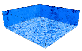
Model. We consider a turbulent Rayleigh-Bénard convection, in which an horizontal fluid layer is heated from below. Horizontal and wall-normal coordinates are indicated by $x_{1}$, $x_{2}$ and $x_{3}$, respectively. Using the Boussinesq approximation, the system is described by the following dimensionless balance equations

$$\frac{\partial u_{i}}{\partial x_{i}} = 0,$$ (1)

$$\frac{\partial u_{i}}{\partial t}+u_{i}\frac{\partial u_{i}}{\partial x_{j}} = -\frac{\partial p}{\partial x_{i}}+4\sqrt{\frac{Pr}{Ra}}\frac{\partial^{2}u_{i}}{\partial x_{j}^{2}}-\delta_{i,3}\theta,$$ (2)

$$\frac{\partial\theta}{\partial t}+u_{i}\frac{\partial\theta}{\partial x_{j}} = +\frac{4}{\sqrt{PrRa}}\frac{\partial^{2}\theta}{\partial x_{j}^{2}},$$ (3)

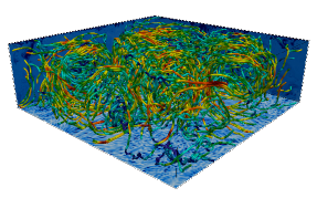
where $u_{i}$ is the $i^{th}$ component of the velocity vector, $p$ is pressure, $\theta=(T-T_{0})/\Delta T$ is the dimensionless temperature, $\Delta T=T_{H}-T_{C}$ is the imposed temperature difference between the hot bottom wall ($T_{H}$) and top cold wall ($T_{C}$), whereas $\delta_{1,3}\theta$ is the driving buoyancy force (acting in the vertical direction $x_{3}$ only). Periodicity is imposed on velocity and temperature along the horizontal directions $x_{1}$ and $x_{2}$, whereas no slip conditions are enforced for velocity at the top and bottom walls. The fluid kinematic viscosity $\nu_{0}$, thermal diffusivity $\kappa_{0}$ and thermal expansion coefficient $\alpha_{0}$ are evaluated at the reference fluid temperature $T_{0}=(T_{H}+T_{C})/2\simeq 29^{o}C$. The Prandtl and the Rayleigh numbers in Eqs. (2)-(3) are defined as $Pr=\nu_{0}/k_{0}$ and $Ra=(g\alpha_{0}\Delta T(2h)^{3})/(\nu_{0}k_{0})$, with $h=0.15\leavevmode\nobreak\ m$ the half domain height and $g$ the acceleration due to gravity. An example of the temperature distribution inside our convection cell is given in Fig. 1a. To measure the local values of the field variables, we make use of a Lagrangian approach. The dynamics of $N_{p}=1.28\cdot 10^{5}$ Lagrangian tracers is computed as

$$\dot{\bf x}_{p}={\bf u}\left({\bf x_{p}}(t),t\right)\leavevmode\nobreak\ \leavevmode\nobreak\ \leavevmode\nobreak\ \leavevmode\nobreak\ \leavevmode\nobreak\ {\theta_{p}}={\theta}\left({\bf x_{p}}(t),t\right),$$ (4)

with ${\bf x_{p}}=(x_{p,1},x_{p,2},x_{p,3})$ the tracers position, $\dot{\bf x}_{p}=(u_{p,1},u_{p,2},u_{p,3})$ their velocity and $\theta_{p}$ their temperature. A visualization of different particle trajectories (colored by the local velocity magnitude) is shown in figure 1b, highlighting also the chaotic nature of the flow.

Fluctuation relation (FR) concerns the symmetry of a representative observable, which is typically linked to the work done on the system, and, through dissipation, to irreversibility. For a Markov process, whose dynamics is described by $\dot{{\bf x}}(t)={\bf u}({\bf x}(t),t)$, the representative observable can be written as Lebowitz and Spohn (1982)

$$\beta W_{t}=\frac{1}{t}\log\frac{\Pi(\{{\bf x}(s)\}_{0}^{t})}{\Pi(\{I{\bf x}(s)\}_{0}^{t})}\leavevmode\nobreak\ ,$$ (5)

where $\{{\bf x}(s)\}_{0}^{t}$ and $\{I{\bf x}(s)\}_{0}^{t}$ are the direct and the time-reversed trajectories in the time interval $[0,t]$ respectively, while $\Pi$ indicates probability and $\beta$ is a suitable energy scale of the system (for small systems $\beta^{-1}=k_{B}T$, with $k_{B}$ the Boltzmann constant and $T$ the absolute temperature of the system). When FR applies,

$$\log\frac{\Pi(\beta W_{t}=p)}{\Pi(\beta W_{t}=-p)}=tp,$$ (6)

where $W_{t}$ is usually called "produced entropy". Note that the choice of a representative observable quantity is crucial to verify the fluctuation relation. Entropy production for a Markov process is usually defined based on the dynamical probability, a quantity that is generally not accessible in complex systems. Previous experimental studies on macroscopic chaotic systems focused on the behavior of the injected power, a measurable quantity that however was found to depart from the predictions given by the FR Farago (2002); Puglisi et al. (2005). In the present case, we start from the balance equation for the turbulent kinetic energy $E_{t}=1/2\langle u^{\prime}_{i}u^{\prime}_{i}\rangle$, where brackets $\langle\rangle$ indicate statistical average and $u^{\prime}_{i}=u_{i}-\langle u_{i}\rangle$ velocity fluctuations. Since the system is homogeneous along the $x_{1}$ and $x_{2}$ directions, we obtain

$$\frac{\partial E_{t}}{\partial t}+\frac{\partial}{\partial x_{3}}(\langle E_{t}u^{\prime}_{3}\rangle+\langle u^{\prime}_{3}p^{\prime}\rangle)=\langle u_{3}^{\prime}\theta^{\prime}\rangle-\langle\epsilon\rangle,$$ (7)

where $\langle\epsilon\rangle=4\sqrt{\frac{Pr}{Ra}}\left(\frac{\partial^{2}\langle E_{t}\rangle}{\partial x^{2}_{3}}+\left\langle\frac{\partial u^{\prime}_{i}}{\partial x_{j}}\frac{\partial u^{\prime}_{i}}{\partial x_{j}}\right\rangle\right)$ is the turbulent dissipation and $\theta^{\prime}$ is the temperature fluctuation. The volume-averaged steady state solution gives $\langle u_{3}^{\prime}\theta^{\prime}\rangle=\langle\epsilon\rangle$. This provides also an estimate of the entropy production, which from thermodynamics is $\langle\epsilon\rangle/\langle T\rangle$. Specifically, we focus on the term $W=\rho_{0}g\alpha_{0}\theta_{p}^{\prime}u^{\prime}_{3,p}$, which we measure along the path of the Lagrangian tracers and that represents the power spent by buoyancy to displace a fluid parcel. Note that $W$ quantifies the vertical flux of energy and is therefore also linked to the vertical Nusselt number Gasteuil et al. (2007); Liot et al. (2015). Warm fluctuations $\theta_{p}^{\prime}>0$ produce a positive energy flux when associated to positive vertical velocities $u_{p,3}>0$, whereas cold fluctuations $\theta_{p}^{\prime}<0$ produce a positive energy flux when associated to negative vertical velocity $u_{p,3}<0$.

We now consider the time-averaged (but fluctuating) expression of the global energy balance of the system, $\Delta U_{\tau}=W_{\tau}+Q_{\tau}$, where

$$W_{\tau}=\frac{1}{\tau}\int_{0}^{\tau}{\bf F}^{ext}(t)\cdot{\bf u}(t)\mathrm{dt}=\frac{1}{\tau}\int_{0}^{\tau}\rho_{0}g\alpha_{0}\theta_{p}^{\prime}u^{\prime}_{p,3}\mathrm{dt}$$ (8)

and ${\bf F^{ext}}$ is the external force field due to gravity, whereas $\Delta U_{\tau}$ and $Q_{\tau}$ indicate internal energy and heat, respectively. In the limit ${\tau}\to\infty$, $\langle\Delta U_{\tau}\rangle=0$ and the energy balance of the system becomes $\langle W_{\tau}\rangle=\langle Q_{\tau}\rangle$. Although work and heat fluctuations are generally different in stochastic systems Van Zon and Cohen (2004), we believe that $W_{\tau}$ can give a good estimate of entropy production.

Results

Figure 2: Lagrangian correlation $R_{W}$ as a function of the time lag $\tau$ for the three different Rayleigh number. The collapse of the correlation function upon rescaling of the time lag $\tau$ by the integral time scale $\tau_{C}$ is explicitly shown in the inset. Note that $\tau_{C}=100\leavevmode\nobreak\ s$ for $Ra=10^{7}$, $\tau_{C}=25\leavevmode\nobreak\ s$ for $Ra=10^{8}$ and $\tau_{C}=7\leavevmode\nobreak\ s$ for $Ra=10^{9}$.

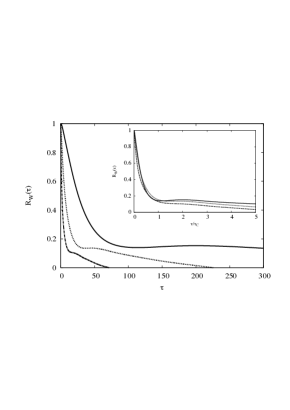
In the following, we will assume that time-averages are equivalent to ensemble averages (ergodicity). This assumption is justified if the correlation function of $W$, $R_{W}=\langle W(t)W(t+\tau)\rangle/\langle W^{2}\rangle$, computed after a statistically steady state is reached, exhibits a fast decrease in time Monin and Yaglom (2007). To verify this, we explicitly compute $R_{W}(\tau)$ for each $Ra$ as a function of the time lag $\tau$. Results are shown in Fig. 2. We observe that $R_{W}$ is characterized by an exponential decay $\exp(-t/\Gamma)$, whose decay rate $1/\Gamma$ increases with increasing $Ra$. As a consequence, velocity and temperature fluctuations decorrelate faster for large $Ra$, due to the larger fluctuations observed for increasing $Ra$. The fast decay of the correlation function happens also in Anosov dynamical systems and in Markov processes, and is a key feature to obtain steady FRMarconi et al. (2008). From the behavior of the correlation function $R_{W}$, we are able to compute the integral correlation time $\tau_{C}=\int_{0}^{\infty}R_{W}(\tau)\mbox{d}\tau$. Upon rescaling of the time lag $\tau$ by $\tau_{C}$, the correlation functions $R_{W}$ computed at different $Ra$ collapse (inset of Fig. 2). For $\tau/\tau_{C}>1$ the value of the correlation is already $R_{W}<0.2$, indicating that from $\tau\simeq\tau_{C}$ the signal is only barely reminiscent of the starting condition. This means that $\tau_{C}$ is a representative time scale of the system and suggests that FR can be conveniently tested for $\tau/\tau_{C}>1$.

Figure 3: Probability density function ($\Pi$) of the normalized energy flux $p=W_{\tau}/\langle W_{\tau}\rangle$ for $Ra=10^{9}$ and for different values of the averaging time window $\tau/\tau_{C}$. The behavior of a Gaussian distribution is explicitly indicated by the solid line. Results from simulations at $Ra=10^{7}$ and $Ra=10^{8}$ are not shown here because they are qualitatively similar to those at $Ra=10^{9}$ and do not add to the discussion.

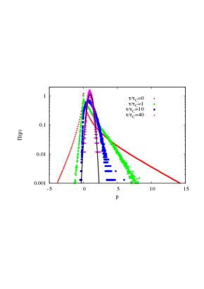
Starting from the Lagrangian measurements of $W$, we compute the probability density function ($\Pi$) of the normalized functional $p=\frac{W_{\tau}}{\langle W_{\tau}\rangle}$ for different values of $\tau$, shown in Fig. 3. For $\tau/\tau_{C}=0$, $\Pi(p)$ is highly asymmetric, with the most probable value occurring for $p=0$ and with positive fluctuations being larger than negative ones. The asymmetry of $\Pi(p)$ persists also for increasing $\tau/\tau_{C}$ and disappears only when the average is done on a rather large time window ($\tau/\tau_{C}\geq 40$). In particular, for $\tau/\tau_{C}\simeq 40$ the distribution peaks around $p\simeq 1$ and recovers an almost gaussian distribution. Note that at this stage ($\tau/\tau_{C}\geq 40$), the probability of negative events becomes essentially zero. These observations suggest that, although the imposed mean temperature difference between the walls induces a net positive vertical energy flux ( $\langle W\rangle>0$), $W$ can often be negative. The occurrence of countegradient fluxes of global transport properties (such as the Nusselt number) is an extremely important phenomenon that has been also observed in other situations Huisman et al. (2012). From a physical point of view, small positive and negative values of $W$ are produced by turbulence, which is uncorrelated with the temperature field. These small positive and negative values of $W$ balance each others and do not contribute to the average heat transport Shang et al. (2005). Only large velocity and temperature fluctuations produced by thermal plumes (rising hot plumes and falling cold plumes) are correlated and contribute to the positive mean heat flux.

It is reasonable to expect that the fluctuations of $p$ are governed by a large deviation law $\Pi(p)\sim e^{\tau\zeta(p)}$, with $\zeta$ concave. Then, from the behavior of $\Pi(p)$, we measure the quantity

$$\zeta(p)-\zeta(-p)=\sigma(p)=\frac{1}{\tau}\log\frac{\Pi(p)}{\Pi(-p)}$$ (9)

for different averaging time $\tau/\tau_{C}$ taken in the range $1<\tau/\tau_{C}<30$. The resulting behavior, given in Fig. 4, nicely shows that $\sigma(p)$ is a linear function of $p$,

$$\sigma(p)=\alpha p.$$ (10)

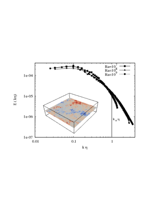
In particular, we observe that the slope $\alpha$ of the curve increases with increasing $Ra$ and tends (for $Ra=10^{9}$) to $\alpha=\beta\langle W_{\tau}\rangle$, as theoretically predicted by the FR. As already mentioned, $\beta$ is a suitable and representative energy scale of the system. Following the Kolmogorov cascade picture Gallavotti (1997); Rondoni and Segre (1999), to study the microscopic nature of the fluctuations we assume that $\beta^{-1}$ is the energy of the dissipative scales $\beta^{-1}=(k_{B}T)_{turb}=1/2\rho\int_{k>k_{R}}E(k)\mbox{d}k$, with $k_{R}$ the wavenumber characterizing dissipation ( i.e. $K_{R}\eta\simeq 1$, with $\eta$ the Kolmogorov lengthscale). The value of $\beta$ is obtained from the turbulent kinetic energy spectrum $E(k)$, as shown in Fig. 5.

Figure 4: Behavior of $(\beta\langle W_{\tau}\rangle)^{-1}\tau^{-1}\log\left(\Pi(p)/\Pi(-p)\right)$ as a function of $p$ for $1<\tau/\tau_{C}<30$, i.e. when the probability density function is not gaussian. Results are shown for each value of the Rayleigh number $Ra$ (as indicated by the arrow). The solid line represents the theoretical prediction given by the FR, a linear function with slope equal to unity. In the inset, the Cramér function $\zeta(p)$, rescaled as suggested by  Rondoni and Morriss (2003) using its standard deviation $\sigma_{\tau}$ and its slope $C_{\tau}$, is shown for different $\tau$ (for $1<\tau<30$). The convergence is satisfying for $\tau>1$.

Figure 5: Time-averaged energy spectra of the turbulent kinetic energy computed at the center of the channel (on the central plane explicitly shown in the inset of the figure, where the flow appears to be homogeneous). The representative energy scale of the system $\beta^{-1}=(k_{B}T)_{turb}=1/2\rho\int_{k>k_{R}}E(k)\mbox{d}k$, computed assuming $k_{R}\eta=1$, gives $\beta=0.49$ for $Ra=10^{7}$, $\beta=0.33$ for $Ra=10^{8}$ and $\beta=0.3$ for $Ra=10^{9}$.

Conclusion In this letter, we have used a Lagrangian approach to study fluctuations of entropy production in turbulent thermal convection. Entropy production has been evaluated from the local measurements of the quantity $W_{\tau}\propto\theta^{\prime}_{p}u^{\prime}_{3,p}$ (work done by buoyancy on fluid particles) along the trajectory of individual Lagrangian tracers. We have shown that $W_{\tau}$ is often negative, and is characterized by fluctuations that follow the FR beyond the linear regime, provided that a representative energy scale for dissipation is suitably identified. This result sheds new light on turbulence, allowing an a priori estimate of the behavior of fluctuations of energy flux or entropy production and giving access to the Cramér function.
We acknowledge Massimo Cencini, Andrea Crisanti and Dario Villamaina for fruitful discussions.

References

- Onsager (1931a) L. Onsager, Physical Review 37, 405 (1931a).
- Onsager (1931b) L. Onsager, Physical Review 38, 2265 (1931b).
- Kubo (1957) R. Kubo, Journal of the Physical Society of Japan 12, 570 (1957).
- Marconi et al. (2008) U. M. B. Marconi, A. Puglisi, L. Rondoni, and A. Vulpiani, Physics reports 461, 111 (2008).
- Evans et al. (1993) D. J. Evans, E. Cohen, and G. Morriss, Physical Review Letters 71, 2401 (1993).
- Evans and Searles (1994) D. J. Evans and D. J. Searles, Phys. Rev. E 50, 1645 (1994).
- Gallavotti and Cohen (1995a) G. Gallavotti and E. Cohen, Physical Review Letters 74, 2694 (1995a).
- Gallavotti and Cohen (1995b) G. Gallavotti and E. Cohen, Journal of Statistical Physics 80, 931 (1995b).
- Jarzynski (1997) C. Jarzynski, Physical Review Letters 78, 2690 (1997).
- Gallavotti (1996) G. Gallavotti, Physical Review Letters 77, 4334 (1996).
- Searles et al. (2007) D. J. Searles, L. Rondoni, and D. J. Evans, Journal of Statistical Physics 128, 1337 (2007).
- Chetrite and Gawedzki (2008) R. Chetrite and K. Gawedzki, Communications in Mathematical Physics 282, 469 (2008).
- Gallavotti (2014) G. Gallavotti, Nonequilibrium and irreversibility (Springer, 2014).
- Ritort (2004) F. Ritort, in Poincaré Seminar 2003 (Springer, 2004) pp. 193–226.
- Ciliberto et al. (2013) S. Ciliberto, R. Gomez-Solano, and A. Petrosyan, Annu. Rev. Condens. Matter Phys. 4, 235 (2013).
- Gallavotti and Lucarini (2014) G. Gallavotti and V. Lucarini, Journal of Statistical Physics 156, 1027 (2014).
- Ciliberto and Laroche (1998) S. Ciliberto and C. Laroche, Le Journal de Physique IV 8, Pr6 (1998).
- Ciliberto et al. (2004) S. Ciliberto, N. Garnier, S. Hernandez, C. Lacpatia, J.-F. Pinton, and G. R. Chavarria, Physica A: Statistical Mechanics and its Applications 340, 240 (2004).
- Falcon et al. (2008) E. Falcon, S. Aumaì̂ tre, C. Falcón, C. Laroche, and S. Fauve, Physical review letters 100, 064503 (2008).
- Cadot et al. (2008) O. Cadot, A. Boudaoud, and C. Touzé, The European Physical Journal B 66, 399 (2008).
- Biferale et al. (1998) L. Biferale, D. Pierotti, and A. Vulpiani, Journal of Physics A: Mathematical and General 31, 21 (1998).
- Gallavotti et al. (2004) G. Gallavotti, L. Rondoni, and E. Segre, Physica D: Nonlinear Phenomena 187, 338 (2004).
- Shang et al. (2005) X.-D. Shang, P. Tong, and K.-Q. Xia, Physical Review E 72, 015301 (2005).
- Zamponi (2007) F. Zamponi, Journal of Statistical Mechanics: Theory and Experiment 2007, P02008 (2007).
- Ruelle (2012) D. P. Ruelle, Proceedings of the National Academy of Sciences 109, 20344 (2012).
- Sekimoto (2010) K. Sekimoto, Stochastic energetics, Vol. 799 (Springer, 2010).
- Toschi and Bodenschatz (2009) F. Toschi and E. Bodenschatz, Annual Review of Fluid Mechanics 41, 375 (2009).
- Puglisi et al. (2005) A. Puglisi, P. Visco, A. Barrat, E. Trizac, and F. van Wijland, Physical review letters 95, 110202 (2005).
- Puglisi and Villamaina (2009) A. Puglisi and D. Villamaina, EPL (Europhysics Letters) 88, 30004 (2009).
- Sarracino et al. (2010) A. Sarracino, D. Villamaina, G. Gradenigo, and A. Puglisi, EPL (Europhysics Letters) 92, 34001 (2010).
- Liot et al. (2015) O. Liot, F. Seychelles, F. Zonta, S. Chibbaro, T. Coudarchet, Y. Gasteuil, J. Pinton, J. Salort, and F. Chilla’, submitted to Journal of Fluid Mechanics - (2015).
- Zonta and Soldati (2014) F. Zonta and A. Soldati, Journal of heat transfer - Trans. ASME 136 (2014).
- Zonta (2013) F. Zonta, International Journal of Heat and Fluid Flow 44, 489 (2013).
- Lebowitz and Spohn (1982) J. Lebowitz and H. Spohn, Journal of Statistical Physics 29, 39 (1982).
- Farago (2002) J. Farago, Journal of statistical physics 107, 781 (2002).
- Gasteuil et al. (2007) Y. Gasteuil, W. Shew, M. Gibert, F. Chilla’, B. Castaing, and J. Pinton, Physical Review Letters 99 (2007).
- Van Zon and Cohen (2004) R. Van Zon and E. Cohen, Physical Review E 69, 056121 (2004).
- Monin and Yaglom (2007) A. S. Monin and A. M. Yaglom, Statistical fluid mechanics: mechanics of turbulence (Dover, 2007).
- Huisman et al. (2012) S. Huisman, D. van Gils, S. Grossmann, C. Sun, and D. Lohse, Physical Review Letters 108 (2012).
- Gallavotti (1997) G. Gallavotti, Physica D: Nonlinear Phenomena 105, 163 (1997).
- Rondoni and Segre (1999) L. Rondoni and E. Segre, Nonlinearity 12, 1471 (1999).
- Rondoni and Morriss (2003) L. Rondoni and G. P. Morriss, Open Systems & Information Dynamics 10, 105 (2003).