The partial copula: Properties and associated dependence measures

Abstract

The partial correlation coefficient is a commonly used measure to assess the conditional dependence between two random variables. We provide a thorough explanation of the partial copula, which is a natural generalization of the partial correlation coefficient, and investigate several of its properties. In addition, properties of some associated partial dependence measures are examined.

Keywords: Partial copula, Conditional copula, Partial correlation, Partial Spearman’s rho, Partial Kendall’s tau.

1 Introduction

Studying the dependence between two random variables $Y_{1}$ and $Y_{2}$ conditional on a random vector $Z$ is an important topic in statistics. The partial correlation coefficient is often used to measure the conditional dependence between two random variables due to its simple computation and meaningful interpretation if the joint distribution of $(Y_{1:2},Z)$ is given by an elliptical distribution. However, outside the elliptical world, the interpretation of the partial correlation coefficient as a measure for conditional dependence is less obvious and can be quite misleading. For instance, it can be zero if there is conditional dependence between two random variables and, even worse, its absolute value can be arbitrarily close to one if two random variables are conditionally independent. The partial copula is a natural generalization of the partial correlation coefficient and gives a meaningful measure of conditional dependence for general distributions. Moreover, there is a large class of distributions where the partial copula completely characterizes the conditional dependence.

We first motivate and define the partial copula in Section 2 and then turn to some examples in Section 3. In Section 4 we take a closer look at the properties of the partial copula. In particular, we examine the optimality of the partial copula as an approximation of the conditional copula and investigate its relation to conditional independence. Section 5 considers dependence measures of the partial copula and how they are related to expected dependence measures of the conditional copula.

2 The partial copula

For simplicity, we consider continuous real-valued random variables with a joint positive density and assume that $\mathbb{E}[Y_{i}]=0$ for $i=1,2$. $Y_{1}\perp Y_{2}|Z$ means that $Y_{1}$ and $Y_{2}$ are independent given $Z$ and $C^{\perp}$ denotes the bivariate product copula. For $i=1,2$, let $\beta_{i}:=\mathbb{E}[ZZ^{\prime}]^{-1}\mathbb{E}[Z^{\prime}Y_{i}]$ so that $Z\beta_{i}$ denotes the best linear predictor of $Y_{i}$ in terms of $Z,$ and define

$${\cal E}_{1}:=Y_{1}-Z\beta_{1},\quad \text{and}\quad{\cal E}_{2}:=Y_{2}-Z\beta_{2}.$$

The partial correlation of $Y_{1}$ and $Y_{2}$ given $Z$ can be expressed as

$$\rho_{Y_{1},Y_{2};Z}=\mathbb{C}\text{orr}[{\cal E}_{1},{\cal E}_{2}].$$

Thus, $\rho_{Y_{1},Y_{2};Z}$ is the correlation of $Y_{1}$ and $Y_{2}$ when each random variable has been corrected for the linear influence of $Z$, i.e., $\mathbb{C}\text{orr}[\tilde{g}({\cal E}_{i}),\tilde{h}(Z)]=0$ for all linear functions $\tilde{g}$ and $\tilde{h}$. If $(Y_{1:2},Z)$ is jointly elliptically distributed, it is well known that $\mathbb{E}[{\cal E}_{1}|Z]=\mathbb{E}[{\cal E}_{2}|Z]=0$ (a.s.), implying that $\rho_{Y_{1},Y_{2};Z}$ describes the dependence of $Y_{1}$ and $Y_{2}$ when their expectation does not depend on $Z$ anymore. Moreover, if the elliptical distribution is a Gaussian distribution, $\rho_{Y_{1},Y_{2};Z}$ completely characterizes the conditional dependence. One reason for that is that ${\cal E}_{1}\perp Z$ and ${\cal E}_{2}\perp Z$, which is equivalent to $\mathbb{C}\text{orr}[h({\cal E}_{i}),g(Z)]=0$ for $i=1,2$, and all measurable functions $h$ and $g$, so that $\rho_{Y_{1},Y_{2};Z}$ can be interpreted as the correlation of random variables which are individually independent of $Z$. In order to generalize this idea to the non-Gaussian case and to obtain random variables which are individually independent of $Z$, we define

$$U_{1}:=F_{Y_{1}|Z}(Y_{1}|Z),\quad \text{and}\quad U_{2}:=F_{Y_{2}|Z}(Y_{2}|Z).$$

$U_{i}$ is called the conditional probability integral transform (CPIT) of $Y_{i}$ wrt $Z$. If $(Y_{1:2},Z)$ has a Gaussian distribution then $U_{i}=\Phi({\cal E}_{i}/\sigma_{{\cal E}_{i}})$ so that $\mathbb{C}\text{orr}[\Phi^{-1}(U_{1}),\Phi^{-1}(U_{2})]=\rho_{Y_{1},Y_{2};Z}$. However, even when the joint distribution of $(Y_{1:2},Z)$ is not Gaussian, we have that $U_{1}\perp Z$ and $U_{2}\perp Z$ (Proposition 2.1 in Spanhel and Kurz (2015)). Thus, dependence measures which are based on the distribution of $(U_{1},U_{2})$ are also meaningful if the underlying distribution is not Gaussian. The joint distribution of the CPITs is the partial copula $C^{\text{\tiny P}}_{Y_{1},Y_{2};Z}$ of $F_{Y_{1},Y_{2}|Z}$ and has been introduced by Bergsma (2011), Gijbels et al. (2015) and Spanhel and Kurz (2015).

In some special cases, e.g., the Gaussian or Student-t distribution (Stöber et al., 2013), the partial copula and the conditional cdfs $(C^{\text{\tiny P}}_{Y_{1},Y_{2};Z},F_{Y_{1}|Z},F_{Y_{2}|Z})$ determine $F_{Y_{1},Y_{2}|Z}$ via $F_{Y_{1},Y_{2}|Z}(y_{1},y_{2}|z)=C^{\text{\tiny P}}_{Y_{1},Y_{2};Z}(u_{1},u_{2})$, where $u_{i}=F_{Y_{i}|Z}(y_{i}|z),i=1,2$. However, in general, we have that $F_{Y_{1},Y_{2}|Z}(y_{1},y_{2}|z)=C_{Y_{1},Y_{2}|Z}(u_{1},u_{2}|z):=\mathbb{P}(U_{1}\leq u_{1},U_{2}\leq u_{2}|Z=z)$, where $C_{Y_{1},Y_{2}|Z}$ denotes the conditional copula of $F_{Y_{1},Y_{2}|Z}$ (Patton, 2006). Thus, the partial copula, which is identical to the expected conditional copula $\int C_{Y_{1},Y_{2};Z}(\cdot,\cdot|t)dF_{Z}(t)$, often acts as an approximation of $C_{Y_{1},Y_{2}|Z}$ or $F_{Y_{1},Y_{2}|Z}$. At first sight, it might appear that the partial copula is a rather rough approximation of $C_{Y_{1},Y_{2}|Z}$ since one assumes that $(U_{1},U_{2})$ are jointly independent of $Z$. However, by construction we have that $U_{1}\perp Z$ and $U_{2}\perp Z$, so these necessary conditions for joint independence are satisfied. In particular, $F_{Y_{1},Y_{2}|Z}$ can be recovered from $(C^{\text{\tiny P}}_{Y_{1},Y_{2};Z},F_{Y_{1}|Z},F_{Y_{2}|Z})$ if and only if $Y_{1}$ and $Y_{2}$ can depend on $Z$ but the remaining dependence between $U_{1}$ and $U_{2}$, which are individually independent of $Z$, does not depend on $Z$. But also when $C^{\text{\tiny P}}_{Y_{1},Y_{2};Z}$ just acts as an approximation of $C_{Y_{1},Y_{2}|Z}$, it is an attractive dependence measure because it is easier to estimate than $C_{Y_{1},Y_{2}|Z}$ and measures conditional dependence by one bivariate unconditional copula and not by infinitely many bivariate unconditional copulas as it is the case for $C_{Y_{1},Y_{2}|Z}$. In the following, we give some explicit examples of partial copulas. Moreover, we investigate to what extent the approximation of $C_{Y_{1},Y_{2}|Z}$ by $C^{\text{\tiny P}}_{Y_{1},Y_{2};Z}$ and the approximation of $F_{Y_{1},Y_{2}|Z}$ by $(C^{\text{\tiny P}}_{Y_{1},Y_{2};Z},F_{Y_{1}|Z},F_{Y_{2}|Z})$ is optimal and examine properties of the partial copula and related dependence measures.

3 Examples of partial copulas

Example 1 (Trivariate FGM copula)

The three-dimensional Farlie-Gumbel-Morgenstern (FGM) copula is given by

$$C_{1:3}(u_{1:3};\theta) =\prod_{i=1}^{3}u_{i}+\theta\prod_{i=1}^{3}u_{i}(1-u_{i}),\quad|\theta|\leq 1.$$

Since this copula is exchangeable, all three conditional copulas $C_{13|2},C_{12|3},C_{23|1}$ are identical. It is straightforward to show that

$$C_{13|2}(u_{1},u_{2}|u_{2}) =\prod_{i=1,3}u_{i|2}+\theta(1-2u_{2})\prod_{i=1,3}u_{i|2}(1-u_{i|2}),$$

and

$$C^{\text{\tiny P}}_{13;2} =C^{\perp}.$$

Example 2 (Trivariate Frank copula)

Consider the exchangeable three-dimensional Frank copula with dependence parameter $\theta>0$,

$$C_{1:3}(u_{1:3}) =\log\left\{1-(1-\alpha)\prod_{i=1}^{3}\frac{1-\alpha^{u_{i}}}{1-\alpha}\right\}\Big{/}\log(\alpha),\quad\alpha:=\exp(-\theta).$$

The conditional copula (Mesfioui and Quessy, 2008) belongs to the Ali-Mikhail-Haq (AMH) family with dependence parameter $\gamma(u_{2};\theta)=1-\exp(-\theta u_{2})$, i.e.,

$$C_{13|2}(u_{1},u_{2}|u_{2}) =\frac{u_{1}u_{2}}{1-\gamma(u_{2};\theta)\prod_{i=1,3}(1-u_{i|2})}.$$

In Section A the closed-form expression for the partial copula is derived, which is given by

$$C^{\text{\tiny P}}_{13;2}(u_{1},u_{2}) =\frac{u_{1}u_{2}}{\theta f(u_{1},u_{2})}\left[\log\big{(}1-(1-\exp(-\theta))(1-f(u_{1},u_{2}))\big{)}+\theta\right]\!,$$

where $f(u_{1},u_{2}):=u_{1}+u_{2}-u_{1}u_{2}$. Figure 1 illustrates $C_{13|2}$ and $C^{\text{\tiny P}}_{13;2}$.

Example 3 (Partial copulas of the Gaussian, Student-t, and Clayton copula)

For the Gaussian, Student-t, and Clayton copula, conditional and partial copulas coincide since the simplifying assumption holds (Stöber et al., 2013).

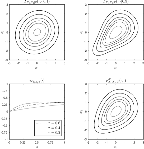
Figure 1: Illustration of the conditional and partial copula if $(Y_{1:2},Z)$ is distributed according to a trivariate Frank copula with pairwise values of Kendall’s $\tau$ being $0.4$. The upper panel shows contour plots of the density of $F_{X_{1},X_{2}|Z}(\cdot,\cdot|z)$ where $X_{i}:=\Phi^{-1}(U_{i})=\Phi^{-1}(F_{Y_{i}|Z}(Y_{i}|Z))$, $i=1,2$, and $\Phi$ is the cdf of the standard normal distribution. On the left hand side in the lower panel the variation of Kendall’s $\tau$ of $C_{Y_{1},Y_{2}|Z}$ is depicted. The lower right figure shows contour plots of the density of $F^{\text{\tiny P}}_{X_{1},X_{2};Z}$.

4 Properties of the partial copula

As stated in Section 2, the partial copula can be considered as an approximation of the conditional copula. The first property shows that the partial copula minimizes the Kullback-Leibler (KL) divergence from the conditional copula.

Property 1 (KL divergence minimization)

The partial copula $C^{\text{\tiny P}}_{Y_{1},Y_{2};Z}$ minimizes the KL divergence from the conditional copula $C_{Y_{1},Y_{2}|Z}$ in the space of absolutely continuous bivariate distribution functions.

Proof:

This follows from equation (3.3) in Theorem 3.1 in Spanhel and Kurz (2015).

However, the partial copula does not always minimize the $L^{2}$ distance to the conditional copula.

Property 2 ($L^{2}$ distance minimization)

Let $C_{Y_{1},Y_{2}|Z}(U_{1},U_{2}|Z)$ have finite variance and ${\cal F}_{2}$ be the space of bivariate cdfs so that each $C_{Y_{1},Y_{2};Z}(U_{1},U_{2})\in{\cal F}_{2}$ is a $C_{Y_{1},Y_{2}|Z}$-measurable random variable with finite variance. Let $C^{L^{2}}_{Y_{1},Y_{2};Z}\in{\cal F}_{2}$ denote the bivariate cdf which minimizes the $L^{2}$ distance to $C_{Y_{1},Y_{2}|Z}$. In general,

$$C^{L^{2}}_{Y_{1},Y_{2};Z} \neq C^{\text{\tiny P}}_{Y_{1},Y_{2};Z}.$$

Proof:

See Section B.

The first two properties address the optimality of the partial copula when it comes to approximating conditional copulas. But partial copulas, together with univariate conditional cdfs, can also be used to provide a model for a general bivariate conditional distribution. For instance, Song et al. (2009) use generalized linear models for univariate conditional cdfs and join these conditional cdfs with an unconditional copula. Also, the conditional cdfs of financial returns are often filtered with ARMA-GARCH models and the remaining dependence is then modeled by an unconditional copula (Chen and Fan, 2006, Liu and Luger, 2009, Min and Czado, 2014, Nikoloulopoulos et al., 2012). Therefore, the next property is of interest if conditional cdfs are linked with the partial copula.

Property 3 (Non-optimality of partial copula-induced approximations)

Let

$$F^{\text{\tiny P}}_{Y_{1},Y_{2}|Z}(y_{1},y_{2}|z):=C^{\text{\tiny P}}_{Y_{1},Y_{2};Z}\big{(}F_{Y_{1}|Z}(y_{1}|z),F_{Y_{2}|Z}(y_{2}|z)\big{)},$$

be the approximation of $F_{Y_{1},Y_{2}|Z}$ that emerges if the conditional copula is approximated by the partial copula and the true univariate conditional cdfs. In general, $F^{\text{\tiny P}}_{Y_{1},Y_{2}|Z}$ does neither minimize the KL divergence nor the $L^{2}$ distance from ${F}_{Y_{1},Y_{2}|Z}$.

Proof:

See Section C.

Although the partial copula $C^{\text{\tiny P}}_{Y_{1},Y_{2};Z}$ minimizes the KL divergence from ${C}_{Y_{1},Y_{2}|Z}$ (Property 1), Property 3 reveals the surprising result that this does not imply that the induced approximation $F^{\text{\tiny P}}_{Y_{1},Y_{2}|Z}$ also minimizes the KL divergence from ${F}_{Y_{1},Y_{2}|Z}$. Note that Property 1 implies that $C^{\text{\tiny P}}_{Y_{1},Y_{2};Z}$ is the bivariate copula that minimizes the KL divergence if the true conditional cdfs $(F_{Y_{1}|Z},F_{Y_{2}|Z})$ are specified. Thus, Property 3 implies that, in general, one can obtain a better approximation by an adequate misspecification of the conditional cdfs. That is, there are conditional cdfs $(\tilde{F}_{Y_{1}|Z},\tilde{F}_{Y_{2}|Z})$ such that $(\tilde{F}_{Y_{1}|Z},\tilde{F}_{Y_{2}|Z})\neq({F}_{Y_{1}|Z},{F}_{Y_{2}|Z})$ and $\mathbb{E}[C^{\text{\tiny P}}_{Y_{1},Y_{2};Z}\big{(}\tilde{F}_{Y_{1}|Z}(Y_{1}|Z),\tilde{F}_{Y_{2}|Z}(Y_{2}|Z)\big{)}]>\mathbb{E}[F^{\text{\tiny P}}_{Y_{1},Y_{2}|Z}(Y_{1},Y_{2}|Z)]$. Because the marginal distributions of $(\tilde{F}_{Y_{1}|Z}(Y_{1}|Z),\tilde{F}_{Y_{2}|Z}(Y_{2}|Z))$ are not uniform in general, one can further improve the approximation if one specifies a pseudo-copula (Fermanian and Wegkamp, 2012). Another interesting implication of Property 3 is that, if the conditional cdfs and the partial copula are estimated, the joint and stepwise ML estimator may have a different probability limit if the partial and conditional copula do not coincide.

Property 4 (Joint and stepwise ML estimation)

Wlog assume that the following random variables and parameters are scalars. Let $(F_{Y_{1}|Z},F_{Y_{2}|Z})$ be the true conditional cdfs and $C^{\text{\tiny P}}_{Y_{1},Y_{2};Z}$ be the true partial copula of $C_{Y_{1},Y_{2}|Z}$. Assume that we observe $n$ independent samples from $(Y_{1:2},Z)$. For $i=1,2,$ let $\tilde{F}_{Y_{i}|Z}(\tilde{\theta}_{i})$ be a parametric conditional cdf and assume that $\exists\theta_{i}\in\Theta_{i}\colon\tilde{F}_{Y_{i}|Z}(\theta_{i})=F_{Y_{i}|Z}$. Let $\tilde{C}_{12}(\tilde{\theta}_{3})$ be a parametric bivariate copula family so that $\exists\theta_{3}\in\Theta_{3}\colon\tilde{C}_{12}(\theta_{3})=C^{\text{\tiny P}}_{Y_{1},Y_{2};Z}$. Let

$$\theta^{J}_{n}:=\operatorname*{arg\,max}_{\tilde{\theta}_{1:3}\in\Theta_{1:3}}\sum_{i=1}^{n}\log\Big{(}\tilde{c}_{12}\big{(}\tilde{F}_{Y_{1}|Z}(Y_{1,i}|Z_{i};\tilde{\theta}_{1}),\tilde{F}_{Y_{2}|Z}(Y_{2,i}|Z_{i};\tilde{\theta}_{2});\tilde{\theta}_{3}\big{)}\prod_{j=1}^{2}\tilde{f}_{Y_{j}|Z}(Y_{j,i}|Z_{i};\tilde{\theta}_{j})\Big{)}$$

be the joint ML estimator and

$$\theta^{S}_{n}:=\begin{pmatrix}\theta_{1:2}^{S}\\ \theta_{3}^{S}\end{pmatrix}=\begin{pmatrix}\displaystyle\operatorname*{arg\,max}_{\tilde{\theta}_{1:2}\in\Theta_{1:2}}\sum_{j=1}^{2}\sum_{i=1}^{n}\log\tilde{f}_{Y_{j}|Z}(Y_{j,i}|Z_{i};\tilde{\theta}_{j})\\ \displaystyle\operatorname*{arg\,max}_{\tilde{\theta}_{3}\in\Theta_{3}}\sum_{i=1}^{n}\log\tilde{c}_{12}\big{(}\tilde{F}_{Y_{1}|Z}(Y_{1,i}|Z_{i};\theta_{1}^{S}),\tilde{F}_{Y_{2}|Z}(Y_{2,i}|Z_{i};\theta_{2}^{S});\tilde{\theta}_{3}\big{)}\end{pmatrix}$$

be the stepwise ML estimator. Assume that the regularity conditions stated in (Joe, 2005) hold and that

$$\gamma:=\operatorname*{arg\,max}_{\tilde{\theta}_{1:3}\in\Theta_{1:3}}\mathbb{E}\Big{[}\log\big{(}\tilde{c}_{12}\big{(}\tilde{F}_{Y_{1}|Z}(Y_{1}|Z;\tilde{\theta}_{1}),\tilde{F}_{Y_{2}|Z}(Y_{2}|Z;\tilde{\theta}_{2});\tilde{\theta}_{3}\big{)}\prod_{j=1}^{2}\tilde{f}_{Y_{j}|Z}(Y_{j}|Z;\tilde{\theta}_{j})\big{)}\Big{]}$$

exists. If $C_{Y_{1},Y_{2}|Z}=C^{\text{\tiny P}}_{Y_{1},Y_{2};Z}$ (a.s.), then $\theta_{n}^{J}\stackrel{{\scriptstyle p}}{{\to}}\theta$ and $\theta_{n}^{S}\stackrel{{\scriptstyle p}}{{\to}}\theta$ for $n\to\infty$. However, if $C_{Y_{1},Y_{2}|Z}\neq C^{\text{\tiny P}}_{Y_{1},Y_{2};Z}$ (a.s.), then $\theta_{n}^{J}\stackrel{{\scriptstyle p}}{{\to}}\gamma$ and $\theta_{n}^{S}\stackrel{{\scriptstyle p}}{{\to}}\theta$ for $n\to\infty$. In particular, $\theta_{i,n}^{J}-\theta_{i,n}^{S}\stackrel{{\scriptstyle p}}{{\to}}0$ may not hold for all $i=1,2,3$.

Proof:

See Section D.

Thus, the well known result that the joint and stepwise ML estimator of conditional cdfs and an unconditional copula converge to the same probability limit may not hold if the partial and conditional copula do not coincide. The next two properties are related to the parametric family of the partial copula.

Property 5 (Archimedean copulas)

Let the copula of $(Y_{1:2},Z)$ be Archimedean. Then $C^{\text{\tiny P}}_{Y_{1},Y_{2};Z}$ might not be Archimedean.

Proof:

See Section E.

Note that, if the copula of $(Y_{1:2},Z)$ is Archimedean, $C_{Y_{1},Y_{2}|Z}$ is always Archimedean (Mesfioui and Quessy, 2008).

Property 6 (Family of the partial copula)

Assume that there is a bivariate parametric copula family $C^{F}(\cdot,\cdot;\theta)$ with parameter $\theta\in\Theta$ and a measurable function $g$ such that $C_{Y_{1},Y_{2}|Z}(\cdot,\cdot,|z)=C^{F}(\cdot,\cdot;g(z))$ for almost all $z$. In general, it does not hold that $\exists\theta\in\Theta:C^{\text{\tiny P}}_{Y_{1},Y_{2};Z}(\cdot,\cdot)=C^{F}(\cdot,\cdot,\theta).$

Proof:

This follows from Property 5.

Thus, partial copulas can also be used to obtain new (unconditional) copulas (see Example 2). One deficiency of the partial correlation coefficient is that its absolute value can be arbitrarily close to one if we have conditional independence. The partial copula is more attractive in this regard as the following property demonstrates.

Property 7 (Conditional (in)dependence)

Let $Y_{1}\perp Y_{2}|Z$. The smallest upper bound for the absolute value of $\rho_{Y_{1},Y_{2};Z}$ is one. However, we always have that $C^{\text{\tiny P}}_{Y_{1},Y_{2};Z}=C^{\perp}$. On the other side, $C^{\text{\tiny P}}_{Y_{1},Y_{2};Z}=C^{\perp}$ or $\rho_{Y_{1},Y_{2};Z}=0$ does not imply that $Y_{1}\perp Y_{2}|Z$.

Proof:

See Section F.

The next property points out that a varying conditional correlation is not sufficient for the non-equality of the partial and conditional copula.

Property 8 (Conditional correlation)

If $\rho_{Y_{1},Y_{2}|Z}(Z)=(\mathbb{E}[Y_{1}Y_{2}|Z]-\mathbb{E}[Y_{1}|Z]\mathbb{E}[Y_{2}|Z])/\sqrt{Var[Y_{1}|Z]Var[Y_{2}|Z]}$ is not almost surely a constant this does not imply that $\mathbb{P}(C_{Y_{1},Y_{2}|Z}=C^{\text{\tiny P}}_{Y_{1},Y_{2};Z})<1$.

Proof:

See Section G.

5 Properties of partial dependence measures

Let $\rho_{C^{\text{\tiny P}}_{Y_{1},Y_{2};Z}},\tau_{C^{\text{\tiny P}}_{Y_{1},Y_{2};Z}},\lambda_{C^{\text{\tiny P}}_{Y_{1},Y_{2};Z}}^{l},$ and $\lambda_{C^{\text{\tiny P}}_{Y_{1},Y_{2};Z}}^{u}$, denote Spearman’s $\rho$, Kendall’s $\tau$, and the corresponding lower and upper tail dependence coefficients of $C^{\text{\tiny P}}_{Y_{1},Y_{2};Z}$. We refer to these dependence measures as partial dependence measures. The next proposition summarizes that partial Spearman’s $\rho$ and the partial tail dependence coefficients are equal to the expected Spearman’s $\rho$ and the expected tail dependence coefficients of the conditional copula.

Property 9 (Partial Spearman’s $\rho$ and partial tail dependence)

It holds that

$$\rho_{C^{\text{\tiny P}}_{Y_{1},Y_{2};Z}} =\mathbb{E}[\rho_{{C}_{Y_{1},Y_{2}|Z}}(Z)]$$

$$\lambda_{C^{\text{\tiny P}}_{Y_{1},Y_{2};Z}}^{l} =\mathbb{E}[\lambda_{{C}_{Y_{1},Y_{2}|Z}}^{l}(Z)]$$

$$\lambda_{C^{\text{\tiny P}}_{Y_{1},Y_{2};Z}}^{u} =\mathbb{E}[\lambda_{{C}_{Y_{1},Y_{2}|Z}}^{u}(Z)]$$

Proof:

These statements are easily verified by computing the expectations.

However, the expected conditional Kendall’s $\tau$ is in general not equal to partial Kendall’s $\tau$.

Property 10 (Partial Kendall’s $\tau$)

In general, $\tau_{C^{\text{\tiny P}}_{Y_{1},Y_{2};Z}}\neq\mathbb{E}[\tau_{C_{Y_{1},Y_{2}|Z}}\left(Z\right)].$

Proof:

See Section H.

Unless $|\rho_{C^{\text{\tiny P}}_{Y_{1},Y_{2};Z}}|=1$, the value of $\rho_{C^{\text{\tiny P}}_{Y_{1},Y_{2};Z}}$ does not provide any information about the value of $\rho_{{C}_{Y_{1},Y_{2}|Z}}$. E.g., $\rho_{C^{\text{\tiny P}}_{Y_{1},Y_{2};Z}}=0$ does not imply that $\rho_{{C}_{Y_{1},Y_{2}|Z}}=0$ (a.s.) (see Example 1). However, for the coefficients of tail dependence we obtain the following relation.

Property 11 (Tail dependence)

$\lambda_{C^{\text{\tiny P}}_{Y_{1},Y_{2};Z}}^{l}=0\Leftrightarrow\lambda_{{C}_{Y_{1},Y_{2}|Z}}^{l}(Z)=0$ (a.s) and $\lambda_{C^{\text{\tiny P}}_{Y_{1},Y_{2};Z}}^{u}=0\Leftrightarrow\lambda_{{C}_{Y_{1},Y_{2}|Z}}^{u}(Z)=0$ (a.s.).

Proof:

Follows by Property 9 and because the coefficients of tail dependence are non-negative.

Thus, the partial copula has no tail dependence if and only if the conditional copula has no tail dependence (a.s.). This is a useful result because we can test for tail dependence of the conditional copula by testing tail dependence of the partial copula. For instance, when modeling a time-varying conditional copula it is important to know whether the time-varying conditional copula should exhibit tail dependence.

6 Concluding remarks

The partial copula is a natural generalization of the partial correlation coefficient which does not share some of its drawbacks. We presented examples of the partial copula and investigated several of its properties. The bivariate partial copula minimizes the KL divergence to a bivariate conditional copula but the resulting approximation of a general bivariate conditional cdf does in general not minimize the KL divergence. As a result, the joint and stepwise ML estimator may converge to different probability limits.

While the partial copula has attractive theoretical properties, its estimation is much more involved than the estimation of the partial correlation coefficient. Non-parametric estimation of the partial copula has been proposed by Gijbels et al. (2015) if there is only one conditioning variable. However, further investigation is required to determine whether such a non-parametric estimator is reasonable if the set of conditioning variables is not very small and we have finite sample sizes. Alternatively, one could use higher-order partial copulas (Spanhel and Kurz, 2015) which constitute a different generalization of the partial correlation coefficient. While higher-order partial copulas do not share all properties of partial copulas, they can be efficiently estimated for a very large set of conditioning variables.

Appendix

A Derivation of the partial Frank copula (Example 2)

Let $g(u_{1},u_{2},\theta):=1-\left(1-\exp\left(-\theta\right)\right)\left(1-u_{1}\right)\left(1-u_{2}\right)$ and $f(u_{1},u_{2}):=u_{1}+u_{2}-u_{1}u_{2}$. The partial copula is given by

$$C^{\text{\tiny P}}_{13;2}\left(u_{1},u_{2}|u_{2}\right) =\int_{0}^{1}C_{13|2}\left(u_{1},u_{2}|u_{2}\right)\text{d}u_{2}=\int_{0}^{1}\frac{u_{1}u_{2}}{1-\left(1-\exp\left(-\theta u_{2}\right)\right)\left(1-u_{1}\right)\left(1-u_{2}\right)}\text{d}u_{2}$$

$$=\int_{1}^{g(u_{1},u_{2},\theta)}\frac{u_{1}u_{2}}{x\theta\left(f(u_{1},u_{2})-x\right)}\text{d}x=\frac{u_{1}u_{2}}{\theta f(u_{1},u_{2})}\int_{1}^{g(u_{1},u_{2},\theta)}\frac{1}{x}-\frac{1}{x-f(u_{1},u_{2})}\text{d}x$$

$$=\frac{u_{1}u_{2}}{\theta f(u_{1},u_{2})}\left[\log\left(x\right)-\log\left(x-f(u_{1},u_{2})\right)\right]_{x=1}^{x=g(u_{1},u_{2},\theta)}=\frac{u_{1}u_{2}}{\theta f(u_{1},u_{2})}\left[\log g(u_{1},u_{2},\theta)+\theta\right].$$

B Proof of Property 2

It is well known that, if the variance of $Y$ exists, $\mathbb{E}[Y|X]$ minimizes the $L^{2}$ distance to $Y$ over all $X$-measurable random variables with finite variance. Thus

$$C^{L2}_{Y_{1},Y_{2};Z}(U_{1},U_{2}) =\operatorname*{\!\!\!\!\!\!\!\!\phantom{{}_{p}}\arg\min\phantom{{}_{p}}\!\!\!\!\!\!\!\!}_{C_{Y_{1},Y_{2};Z}\in{\cal F}_{2}}\mathbb{E}\big{[}(C_{Y_{1},Y_{2}|Z}(U_{1},U_{2}|Z)-C_{Y_{1},Y_{2};Z}(U_{1},U_{2}))^{2}\big{]}=\mathbb{E}\big{[}C_{Y_{1},Y_{2}|Z}(U_{1},U_{2}|Z)|U_{1},U_{2}\big{]}.$$

It is easy to check that $C^{L^{2}}_{Y_{1},Y_{2};Z}$ is a bivariate copula. If $C_{Y_{1},Y_{2},Z}$ is the FGM copula given in Example 1 then

$$C_{Y_{1},Y_{2};Z}^{L^{2}}(u_{1},u_{2}) =\int_{0}^{1}C_{Y_{1},Y_{2}|Z}(u_{1},u_{2}|z)f_{Z|U_{1},U_{2}}(z|u_{1},u_{2})dz$$

$$=u_{1}u_{2}\left(1+\frac{\theta^{2}(4u_{1}^{2}u_{2}^{2}-6(u_{1}^{2}u_{2}+u_{1}u_{2}^{2})+2(u_{1}^{2}+u_{2}^{2})+9u_{1}u_{2}-3(u_{1}+u_{2})+1)}{3}\right)$$

$$\neq u_{1}u_{2}=C^{\text{\tiny P}}_{Y_{1},Y_{2};Z}(u_{1},u_{2}).$$

C Proof of Property 3

Wlog assume that $Z$ is a scalar and that $(Y_{1},Y_{2},Z)$ is a uniform random vector with $(Y_{1},Z)\sim C_{12}$ and $(Z,Y_{2})\sim C_{23}$. The KL divergence of $\tilde{F}_{Y_{1},Y_{2}|Z}$ from $F_{Y_{1},Y_{2}|Z}$ is given by

$$D_{KL}(F_{Y_{1},Y_{2}|Z},\tilde{F}_{Y_{1},Y_{2}|Z}) =\mathbb{E}\left[\log\frac{f_{Y_{1},Y_{2}|Z}(Y_{1},Y_{2}|Z)}{\tilde{f}_{Y_{1},Y_{2}|Z}(Y_{1},Y_{2}|Z)}\right]$$

and is identical to the KL divergence given in equation (3.1) in Spanhel and Kurz (2015). From equation (3.7) in Theorem 3.2 in Spanhel and Kurz (2015) it follows that $D_{KL}(F_{Y_{1},Y_{2}|Z},\tilde{F}_{Y_{1},Y_{2}|Z})$ does, in general, not attain a minimum at $\tilde{F}_{Y_{1},Y_{2}|Z}=F^{\text{\tiny P}}_{Y_{1},Y_{2}|Z}$. That $F^{\text{\tiny P}}_{Y_{1},Y_{2}|Z}$ may not minimize the $L^{2}$ distance to $F_{Y_{1},Y_{2}|Z}$ follows from Property 2.

D Proof of Property 4

Joe (2005) establishes regularity conditions so that, if $C_{Y_{1},Y_{2}|Z}=C^{\text{\tiny P}}_{Y_{1},Y_{2};Z}$ (a.s.), then $\theta_{n}^{S}\stackrel{{\scriptstyle p}}{{\to}}\theta$ and $\theta_{n}^{J}\stackrel{{\scriptstyle p}}{{\to}}\theta$, which implies that $\theta_{n}^{J}-\theta_{n}^{S}\stackrel{{\scriptstyle p}}{{\to}}0$ holds. Now, let $C_{Y_{1},Y_{2}|Z}\neq C^{\text{\tiny P}}_{Y_{1},Y_{2};Z}$ and assume that $\gamma=\operatorname*{arg\,max}_{\tilde{\theta}_{1:3}\in\Theta_{1:3}}\mathbb{E}\big{[}\log\big{(}\tilde{c}_{12}\big{(}\tilde{F}_{Y_{1}|Z}(Y_{1}|Z;\tilde{\theta}_{1}),\tilde{F}_{Y_{2}|Z}(Y_{2}|Z;\tilde{\theta}_{2});\tilde{\theta}_{3}\big{)}\prod_{j=1}^{2}\tilde{f}_{Y_{j}|Z}(Y_{j}|Z;\tilde{\theta}_{j})\big{)}\big{]}$ exists. Note that, $\displaystyle\theta_{1:2}=\operatorname*{arg\,max}_{\tilde{\theta}_{12}\in\Theta_{12}}\mathbb{E}\big{[}\sum_{j=1}^{2}\log\tilde{f}_{Y_{j}|Z}(Y_{j}|Z;\tilde{\theta}_{j})\big{]}$ and $\displaystyle\theta_{3}=\operatorname*{arg\,max}_{\tilde{\theta}_{3}\in\Theta_{3}}\mathbb{E}\big{[}\log\tilde{c}_{12}\big{(}\tilde{F}_{Y_{1}|Z}(Y_{1}|Z;\theta_{1}),\tilde{F}_{Y_{2}|Z}(Y_{2}|Z;\theta_{2});\tilde{\theta}_{3}\big{)}\big{]}$. Thus, under the regularity conditions in Joe (2005), it follows that $\theta^{S}_{n}\stackrel{{\scriptstyle p}}{{\to}}\theta$. Property 3 and the subsequent remarks imply that, in general, $\gamma_{i}\neq\theta_{i}$ for all $i=1,2,3$. Provided the regularity conditions in Joe (2005) are satisfied, it follows that $\theta^{J}_{i,n}\stackrel{{\scriptstyle p}}{{\to}}\gamma_{i}$ for all $i=1,2,3$, which finishes the proof.

E Proof of Property 5

Let $C^{\text{\tiny P}}_{Y_{1},Y_{2};Z}$ be given as in Example 2. We observe that

$$C^{\text{\tiny P}}_{13;2}\big{(}C^{\text{\tiny P}}_{13;2}(0.25,0.5),0.5\big{)}\neq C^{\text{\tiny P}}_{13;2}\big{(}0.25,C^{\text{\tiny P}}_{13;2}(0.5,0.5)\big{)},$$

which shows that $C^{\text{\tiny P}}_{13;2}$ is not associative, which is sufficient for the copula not to be Archimedean (Nelsen, 2006).

F Proof of Property 7

Let $Z\sim N(0,1)$ and $Y_{1}=-1+Z^{2}+{\cal E}_{1},Y_{2}=-1+Z^{2}+{\cal E}_{2}$, where ${\cal E}_{1},{\cal E}_{2}$, and $Z$ are mutually independent, $\mathbb{E}[{\cal E}_{i}]=0$ and $\mathbb{V}\text{ar}[{\cal E}_{i}]=\sigma$ for $i=1,2$. It is easy to show that $Y_{1}\perp Y_{2}|Z$. Note that $\mathbb{C}\text{ov}[Y_{i},Z]=\mathbb{E}[Z^{3}]=0$ so that $Y_{i}-(1,Z)\beta_{i}=Z^{2}+{\cal E}_{i}$, where $\beta_{i}$ is the best linear predictor of $Y_{i}$ in terms of $Z$. Thus, $\rho_{Y_{1},Y_{2};Z}=\mathbb{C}\text{orr}[Z^{2}+{\cal E}_{1},Z^{2}+{\cal E}_{2}]=\frac{\mathbb{V}\text{ar}[Z^{2}]}{\mathbb{V}\text{ar}[Z^{2}]+\sigma}$, and $\lim_{\sigma\to 0}\rho_{Y_{1},Y_{2};Z}=1$. Setting $Y_{2}=-Z^{2}+{\cal E}_{2}$ shows that $\lim_{\sigma\to 0}\rho_{Y_{1},Y_{2};Z}=-1$. If $Y_{1}\perp Y_{2}|Z$ then $C_{Y_{1},Y_{2}|Z}(U_{1},U_{2}|Z)=U_{1}U_{2}$, i.e., $C^{\text{\tiny P}}_{Y_{1},Y_{2};Z}=C^{\perp}$. From Example 1 it follows that $C^{\text{\tiny P}}_{Y_{1},Y_{2};Z}=C^{\perp}$ does not imply that $Y_{1}\perp Y_{2}|Z$.

G Proof of Property 8

Let $Z$ be exponentially distributed with unit mean, $Y_{1}|Z\sim\log{\cal N}(0,1)$ and $Y_{2}|Z=z\sim\log{\cal N}(0,z)$, where $\log{\cal N}(0,\sigma)$ denotes the log-normal distribution with zero location parameter and scale parameter $\sigma$. Using the same arguments as in Example 5.26 in McNeil et al. (2005), we obtain that, if $C_{Y_{1},Y_{2}|Z}(U_{1},U_{2}|Z)=\min(U_{1},U_{2})=C^{\text{\tiny P}}_{Y_{1},Y_{2};Z}$, the support of the random variable

$$\rho_{Y_{1},Y_{2}|Z}(Z)=\frac{\exp(Z)-1}{\sqrt{(\exp(1)-1)(\exp(Z^{2})-1)}}$$

is the unit interval $[0,1]$.

H Proof of Property 10

Let $Z$ be uniformly distributed and consider the following conditional copula

$$C_{Y_{1},Y_{2}|Z}\left(u_{1},u_{2}|z\right) =u_{1}u_{2}+zu_{1}u_{2}\left(1-u_{1}\right)\left(1-u_{2}\right)(1+u_{1}u_{2}).$$

The corresponding partial copula is

$$C^{\text{\tiny P}}_{Y_{1},Y_{2};Z}(u_{1},u_{2}) =u_{1}u_{2}+\frac{1}{2}u_{1}u_{2}\left(1-u_{1}\right)\left(1-u_{2}\right)(1+u_{1}u_{2}).$$

Elementary integration yields that Kendall’s $\tau$ for the conditional copula is given by

$$\tau_{C_{Y_{1},Y_{2}|Z}}\left(Z\right) =4\int_{\left[0,1\right]^{2}}C_{Y_{1},Y_{2}|Z}\left(u_{1},u_{2}|Z\right)dC_{Y_{1},Y_{2}|Z}\left(u_{1},u_{2}|Z\right)-1=Z^{2}/450+5Z/18$$

Thus,

$$\mathbb{E}[\tau_{C_{Y_{1},Y_{2}|Z}}\left(Z\right)] =\frac{377}{2700}\neq\frac{251}{1800}=\tau_{C^{\text{\tiny P}}_{Y_{1},Y_{2};Z}}.$$

References

• Bergsma (2011) Bergsma, W., 2011. Nonparametric testing of conditional independence by means of the partial copula. ArXiv e-prints arXiv:1101.4607.
• Chen and Fan (2006) Chen, X., Fan, Y., 2006. Estimation and model selection of semiparametric copula-based multivariate dynamic models under copula misspecification. Journal of Econometrics 135, 125--154.
• Fermanian and Wegkamp (2012) Fermanian, J.D., Wegkamp, M.H., 2012. Time-dependent copulas. Journal of Multivariate Analysis 110, 19--29.
• Gijbels et al. (2015) Gijbels, I., Omelka, M., Veraverbeke, N., 2015. Estimation of a copula when a covariate affects only marginal distributions. Scandinavian Journal of Statistics 42, 1109--1126.
• Joe (2005) Joe, H., 2005. Asymptotic efficiency of the two-stage estimation method for copula-based models. Journal of Multivariate Analysis 94, 401 -- 419.
• Liu and Luger (2009) Liu, Y., Luger, R., 2009. Efficient estimation of copula-GARCH models. Computational Statistics & Data Analysis 53, 2284--2297.
• McNeil et al. (2005) McNeil, A.J., Frey, R., Embrechts, P., 2005. Quantitative risk management. Princeton series in finance, Princeton Univ. Press, Princeton NJ.
• Mesfioui and Quessy (2008) Mesfioui, M., Quessy, J.F., 2008. Dependence structure of conditional Archimedean copulas. Journal of Multivariate Analysis 99, 372--385.
• Min and Czado (2014) Min, A., Czado, C., 2014. SCOMDY models based on pair-copula constructions with application to exchange rates. Computational Statistics & Data Analysis 76, 523--535.
• Nelsen (2006) Nelsen, R.B., 2006. An introduction to copulas. Springer series in statistics, Springer, New York.
• Nikoloulopoulos et al. (2012) Nikoloulopoulos, A.K., Joe, H., Li, H., 2012. Vine copulas with asymmetric tail dependence and applications to financial return data. Computational Statistics & Data Analysis 56, 3659--3673.
• Patton (2006) Patton, A.J., 2006. Modelling Asymmetric Exchange Rate Dependence. International Economic Review 47, 527--556.
• Song et al. (2009) Song, P.X.K., Li, M., Yuan, Y., 2009. Joint Regression Analysis of Correlated Data Using Gaussian Copulas. Biometrics 65, 60--68.
• Spanhel and Kurz (2015) Spanhel, F., Kurz, M.S., 2015. Simplified vine copula models: Approximations based on the simplifying assumption. ArXiv e-prints arXiv:1510.06971.
• Stöber et al. (2013) Stöber, J., Joe, H., Czado, C., 2013. Simplified pair copula constructions---Limitations and extensions. Journal of Multivariate Analysis 119, 101--118.