Exactly solvable Wadati potentials in the PT-symmetric Gross-Pitaevskii equation

Abstract

This note examines Gross-Pitaevskii equations with PT-symmetric potentials of the Wadati type: $V=-W^{2}+iW_{x}$. We formulate a recipe for the construction of Wadati potentials supporting exact localised solutions. The general procedure is exemplified by equations with attractive and repulsive cubic nonlinearity bearing a variety of bright and dark solitons.

1 Introduction

A mean-field description of bosons with pairwise interaction is furnished by the Gross-Pitaevskii equation. In the one-dimensional geometry, the equation reads

$$i\,\Psi_{t}+\Psi_{xx}-V(x)\Psi+g\Psi|\Psi|^{2}=0.$$ (1)

In this contribution, we will be concerned with the Gross-Pitaevskii equations featuring complex potentials $V(x)$ Muga ; Moiseev . In quantum physics, complex potentials provide a simple means to account for the inelastic scattering of particles as well as for the loading of particles in an open system Cartarius ; Cartarius1 . The $x$-intervals with $\mathrm{Im}\,V(x)>0$ and $\mathrm{Im}\,V(x)<0$ correspond to the gain and loss of particles, respectively. When the gain exactly compensates the loss, that is, when $V$ obeys the symmetry

$$V^{*}(x)=V(-x),$$ (2)

the potential is referred to as the parity-time (PT-) symmetric Bender .

The nonlinear Schrödinger equation (1) with a PT-symmetric potential (2) is also used in the paraxial nonlinear optics Ziad . In the optics contest, $t$ and $x$ stand for the longitudinal and transverse coordinates, and $V(x)$ models the complex refractive index Muga2 .

Stimulated by the interest from the atomic physics and optics, a number of exactly-solvable Gross-Pitaevskii equations was identified, both within and outside the PT-symmetric variety. The list includes periodic complex potentials Musslimani2 ; AKSY ; the PT-symmetric Scarff II Ziad ; Shi and Rosen-Morse II potentials Midya , as well as a PT-symmetric double-well superposition of a quadratic and a gaussian Midya2 .

This contribution deals with potentials of the form

$$V(x)=-W^{2}+iW_{x},$$ (3)

where $W(x)$ is a real function (called the potential base below), with $W(x)\to\mathrm{const}$ as $|x|\to\infty$. Wadati was apparently the first who noted the relevance of potentials (3) for the PT-symmetric quantum mechanics Wadati . For the purposes of this study, we will be referring to (3) as the Wadati potentials.

We consider the standing-wave solutions $\Psi(x,t)=\psi(x)e^{i\kappa^{2}t}$, where $\kappa^{2}$ is real while the spatial part of the eigenfunction obeys the stationary equation

$$-\psi_{xx}+V(x)\psi-g\psi|\psi|^{2}=-\kappa^{2}\psi.$$ (4)

In the linear case ($g=0$), the stationary Schrödinger equation with the potential (3) and eigenvalue $-\kappa^{2}$ can be mapped onto the Zakharov-Shabat spectral problem, with the potential $W(x)$ and eigenvalue $i\kappa$ Wadati74 ; Andrianov99 ; Lamb . This correspondence allows one to obtain complex Schrödinger potentials with an entirely real spectrum from the real Zakharov-Shabat potentials whose entire discrete spectrum is pure imaginary. Potentials of the latter type are abundant — in fact, all Zakharov-Shabat eigenvalues of any single-peaked real potential $W(x)$ are pure imaginary Klaus02 ; FatkOL14 . An example of a multihump potential with an entirely imaginary discrete spectrum is given by the modified Korteweg-de Vries multisoliton Wadati82 .

In the nonlinear domain, the Gross-Pitaevskii equations with Wadati potentials enjoy an equally exceptional status. In the context of systems with gain and loss, the PT-symmetric Wadati potentials are unique among all PT-symmetric potentials in supporting continuous families of asymmetric solitons Yang14d . This feature has an analogue outside the realm of PT-symmetric systems. Namely, unlike the generic non-PT symmetric potentials, the PT-asymmetric Wadati potentials bear continuous families of stable nonlinear modes FatkOL14 ; KZ14b . (Generic non-PT symmetric complex potentials can only support isolated dissipative solitons rather than continuous families of those AA05 .) These unique attributes of the Wadati potentials stem from the fact that the stationary nonlinear Schrödinger equation (4) with $V$ as in (3) has an $x$-independent invariant KZ14b .

Finally, it is fitting to note that the Wadati potentials support constant-density waves. This property has been used to study the modulational instability within the Gross-Pitaevskii equations with complex potentials MMCR15 .

In this contribution we propose a new procedure for the systematic construction of exactly solvable Wadati potentials. Here, we restrict ourselves to the PT-symmetric case, that is, to the even functions $W(x)$.

Our approach is formulated in sections 2 and 4 for the attractive ($g>0$) and repulsive ($g<0$) boson gas, respectively. The general procedure for the attractive nonlinearity is exemplified by two Wadati potentials with exact bright solitons (section 3). In the repulsive-gas situation, we construct potentials bearing exact lump and bubble solutions (section 5). Finally, section 6 presents a Wadati potential generating a stationary flow of the condensate.

2 General procedure: attractive nonlinearity

We start with the attractive nonlinearity, $g>0$, and assume that the potential has been gauged so that $W_{x}\to 0$ as $|x|\to\infty$. Our main interest is in localised solutions; these obey

$$|\psi(x)|\to 0,\ |\psi_{x}(x)|\to 0\quad\text{as}\ |x|\to\infty.$$ (5)

The boundary conditions (5) require that $\kappa^{2}>0$. We let $\kappa>0$, for definiteness.

It is convenient to cast the equation (4) in the form

$$u_{zz}+(A^{2}-iA_{z})u+2u|u|^{2}=u,$$ (6)

where

$$A(z)=\frac{W(x)}{\kappa},\quad u(z)=\sqrt{\frac{g}{2}}\frac{\psi(x)}{\kappa},\quad z=\kappa x.$$

The boundary conditions (5) translate into

$$|u(z)|\to 0,\ |u_{z}|\to 0\quad\text{as}\ |z|\to\infty.$$ (7)

Central to our approach is the observation that the equation (6) can be written as a first-order system

$$u_{z}- iAu+v=0,$$

$$v_{z}+ iAv-2u|u|^{2}+u=0.$$

The polar decomposition

$$u=ae^{i\theta},\quad v=be^{i\chi},$$

where $a>0$, $0\leq\theta<2\pi$ and $b^{2}>0$, $0\leq\chi<\pi$, takes this system to

$$a_{z} =-b\cos\mu,$$ (8a)

$$b_{z} =a({2}a^{2}-1)\cos\mu,$$ (8b)

$$(\theta_{z}-A)a =-b\sin\mu,$$ (8c)

$$(\chi_{z}+A)b =a(1-{2}a^{2})\sin\mu,$$ (8d)

where we have introduced the angle

$$\mu(z)=\chi(z)-\theta(z).$$

An immediate consequence of equations (8a)-(8b) is a conservation law

$$a^{2}\left(1-a^{2}\right)=b^{2}+C,$$

where $C$ is a constant. Equation (8c), along with the boundary conditions (7) and the fact that $A$ remains bounded as $|z|\to\infty$, gives $b\sin\mu\to 0$. On the other hand, equation (8a) implies $b\cos\mu\to 0$. Taken together, these two results lead us to conclude that $b\to 0$ as $|z|\to\infty$ and so $C=0$:

$$a^{2}\left(1-a^{2}\right)=b^{2}.$$ (9)

With the relation (9) in place, equation (8a) can be integrated to give

$$a={\rm sech}(\Phi-\Phi_{0}),\quad b={\rm sech}(\Phi-\Phi_{0}){\rm tanh}(\Phi-\Phi_{0}),$$ (10)

where

$$\Phi(z)=\int_{0}^{z}\cos\mu(s)ds,$$

and $\Phi_{0}$ is a constant of integration. The remaining two equations, (8c) and (8d), can be solved for $\theta$ and $A$:

$$\theta=-\frac{\mu}{2}-\frac{1}{2}\int\frac{a^{3}}{b}\sin\mu dz,$$ (11)

$$A=-\frac{\mu_{z}}{2}+\frac{a}{2b}\left(2-3a^{2}\right)\sin\mu.$$ (12)

The seed function $\cos\mu(z)$ can be chosen arbitrarily. Once $\mu(z)$ has been chosen, the first equation in (10) gives $a(z)$ while equation (11) together with the second equation in (10) produce $\theta(z)$. The corresponding potential base function $A(z)$ is given by (12).

In this contribution we confine ourselves to the seed functions whose integrals $\Phi(z)$ are bounded (from above or from below) over the whole line. Assuming, for definiteness, that $\Phi(z)$ is bounded from below and choosing the constant $\Phi_{0}$ to satisfy

$$\Phi_{0}<\inf_{-\infty<z<\infty}\Phi(z),$$

we will ensure that $\Phi(z)-\Phi_{0}>0$ and the function $b(z)$ in (10) is bounded away from zero. Then the quotient $a(z)/b(z)$ in (11) and (12) will be nonsingular:

$$\left|\frac{a}{b}\right|={\rm cotanh}\left|\Phi(z)-\Phi_{0}\right|<\infty.$$

A simple class of suitable $\Phi(z)$ consists of even functions bounded by their value at the origin.

Finally, equation (10) implies that the solution will only be localised (that is, satisfy the boundary conditions (7)) if the integral $\int_{-\infty}^{\infty}\cos\mu\,ds$ diverges. This means that $\cos\mu(z)$ should either remain nonzero as $|z|\to\infty$ (for example, tend to a nonzero constant), or decay to zero — but no faster than $z^{-1}$.

3 Pulse-like solitons: two simple examples

As our first example we take the seed function of the form

$$\cos\mu(z)=\frac{\sinh z}{\sqrt{\sinh^{2}z+\cos^{2}\alpha}},$$ (13)

where $0\leq\alpha<\pi/2$ is a parameter. The corresponding integral

$$\Phi(z)={\rm Arctanh}\sqrt{1-\sin^{2}\alpha\,\mathrm{sech}^{2}z}$$ (14)

is even and monotonically growing from ${\rm Arctanh}(\cos\alpha)$ to infinity as $z$ varies from 0 to $\infty$. We let $\Phi_{0}=0$, for simplicity.

Equations (10), (11), and (12) give the potential base function

$$A=\frac{3}{2}\cos{\alpha}\,\mathrm{sech}\,z,$$ (15)

as well as the absolute value and phase of the soliton:

$$a=\sin\alpha\,\mathrm{sech}\,z,\quad\theta=\frac{1}{2}\cos\alpha\arctan\left(\sinh\,z\right).$$ (16)

The Wadati potential $-A^{2}+iA_{z}$ with $A$ as in (15) belongs to the class of PT-symmetric potentials considered by Musslimani et al Ziad , and equations (16) constitute their soliton solution.

Our second example is equally simple — yet new. This time the seed function is

$$\cos\mu(z)=\frac{1}{\sqrt{1+z^{2}}},$$

with the integral

$$\Phi(z)={\rm Arctanh}\frac{z}{\sqrt{1+z^{2}}}.$$

The function $\Phi(z)$ grows without bound as $z$ changes from zero to infinity. Making use of equations (10), (11), and (12) we arrive at the base

$$A(z)=1-\frac{2}{1+z^{2}}$$

and the corresponding PT-symmetric complex Wadati potential:

$$-A^{2}+iA_{z}=-1+\frac{4z(z+i)}{(z^{2}+1)^{2}}.$$ (17)

The localised nonlinear mode, or the soliton, supported by this potential is also given by a rational function:

$$u(z)=\frac{1-iz}{1+z^{2}}.$$ (18)

(We remind the reader that $z$ is a real coordinate in (17) and (18).)

The potential (17) and the soliton (18) are depicted in Fig. 1.

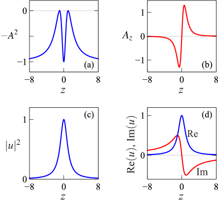
Figure 1: Top row: the real (a) and imaginary (b) part of the rational-function PT-symmetric potential (17). Bottom row: the modulus squared of the corresponding localised nonlinear mode (c) and its real and imaginary part (d).

4 Repulsive nonlinearity and nonvanishing backgrounds

Turning to the Gross-Pitaevskii equation with repulsion (equation (4) with $g<0$), we focus on solitons in the constant-density condensate, that is, localised solutions satisfying the nonvanishing boundary conditions at infinity:

$$|\psi(x)|^{2}\to\rho_{0},\,|\psi_{x}(x)|\to 0\quad\text{as}\ |x|\to\infty.$$ (19)

Assuming that the potential has been gauged so that $W(x)\to 0$ as $|x|\to\infty$, the conditions (19) require $\kappa^{2}=g\rho_{0}<0$. Scaling the dependent and independent variables as in

$$A(z)=\lambda W(x),\quad u(z)=\sqrt{-\frac{g}{2}}\lambda\psi(x),\quad z=\frac{x}{\lambda},$$

with $\lambda=\sqrt{-2/\kappa^{2}}>0$, the equation (4) becomes

$$u_{zz}+(A^{2}-iA_{z})u-2u|u|^{2}=-2u,$$ (20)

while the nonvanishing boundary conditions are reduced to

$$|u|^{2}\to 1,\ |u_{z}|^{2}\to 0\quad\text{as}\ |z|\to\infty.$$ (21)

The equation (20) can be written as a first-order system

$$u_{z}- iAu+v=0,$$ (22)

$$v_{z}+ iAv+2u|u|^{2}-2u=0.$$ (23)

In the same way as the system (8a)-(8b) gave rise to the conservation law (9), the system (22)-(23) implies

$$b=\pm(1-a^{2}),$$ (24)

where we have introduced the polar decomposition

$$u=ae^{i\theta},\quad v=be^{i\chi},$$

and used the boundary conditions (21) together with the fact that $A\to 0$ at infinity. In (24), the top sign corresponds to solutions with $a\leq 1$ while the bottom sign pertains to those with $a\geq 1$.

Letting $\mu(z)=\chi(z)-\theta(z)$ and making use of the conservation law (24) we obtain the modulus and phase of the solution in the sector $a\leq 1$:

$$a=-\tanh(\Phi-\Phi_{0}),\quad\theta=-\frac{\mu}{2}-\int\frac{(a^{2}+1)}{2a}\sin\mu\,dz.$$ (25)

Here

$$\Phi(z)=\int_{0}^{z}\cos\mu(s)ds,$$

as before. The Wadati potential bearing the solution (25) is based on the function

$$A=-\frac{\mu_{z}}{2}+\frac{(1-3a^{2})}{2a}\sin\mu.$$ (26)

In the sector $a\geq 1$, the potential base and solution are given by

$$A=-\frac{\mu_{z}}{2}+\frac{(3a^{2}-1)}{2a}\sin\mu;$$

$$a=\mathrm{cotanh}(\Phi-\Phi_{0}),\quad\theta=-\frac{\mu}{2}+\int\frac{(a^{2}+1)}{2a}\sin\mu\,dz.$$

5 Lumps and bubbles in a homogeneous condensate

Consider, first, the case $a\leq 1$ and let

$$\cos\mu(z)=-\frac{\sinh z}{\sqrt{\sinh^{2}z+\cos^{2}\alpha}},$$ (27)

where $0\leq\alpha<\pi/2$ is a parameter. (This is a negative of the seed function (13) employed in the attractive case.) Using the integral

$$\Phi(z)=-{\rm Arctanh}\,\sqrt{1-\sin^{2}\alpha\,\mathrm{sech}^{2}z}$$

and letting $\Phi_{0}=0$, equation (26) provides the potential base:

$$A=\frac{3\cos\alpha}{2}\,\mathrm{sech}\,z.$$ (28)

Equations (25) give the corresponding solution:

$$u=(\cos\alpha\,\mathrm{sech}\,z+i\tanh z)(\mathrm{sech}\,z+i\tanh z)^{\sigma},\quad\sigma=\frac{\cos\alpha}{2}.$$ (29)

The quantity $|u|^{2}$ has a dip at the origin:

$$|u|^{2}=1-\sin^{2}{\alpha}\,\mathrm{sech}^{2}z.$$

Therefore, equation (29) describes a bubble — a localised rarefaction in a homogeneous background density.

In the sector $a\geq 1$, choosing

$$\cos\mu(z)=\frac{\sinh z}{\sqrt{\sinh^{2}z+\cosh^{2}\beta}},\quad\Phi(z)={\rm Arccoth}\sqrt{1+\sinh^{2}\beta\,\mathrm{sech}^{2}z},$$

with $\beta$ a real parameter, $0\leq\beta<\infty$, gives rise to the potential base

$$A=\frac{3\cosh\beta}{2}\mathrm{sech}\,z$$ (30)

and the solution

$$u=(\cosh\beta\,\mathrm{sech}\,z+i\tanh z)(\mathrm{sech}\,z+i\tanh z)^{\sigma},\quad\sigma=\frac{\cosh\beta}{2}.$$

This time the quantity $|u|^{2}$ has a maximum at the origin,

$$|u|^{2}=1+\sinh^{2}\beta\,\mathrm{sech}^{2}z,$$

and so the solution describes a lump — a localised domain of compression in a condensate of uniform density.

Note that the potential base (28) can be formally obtained from (30) by letting $\beta=i\alpha$. Therefore the bubble- and lump-like solitons form a seamless one-parameter family.

6 Solitons in a stationary flow

In the boson-condensate interpretation of solutions to the equation (6), the function $J(z)=a^{2}\theta_{z}$ represents the superfluid current. Physically, of interest are stationary flows, that is, solutions with $J(z)$ approaching nonzero values as $z\to\pm\infty$. In this section we construct Wadati potentials supporting the stationary flow of condensate.

The lump and the bubble solitons from the previous section are characterised by the zero current at infinity. To construct exact solutions with a nonzero stationary current, we modify the seed function (27) by introducing an additional parameter:

$$\cos\mu=-\sin\varphi\,\frac{\sinh y}{\sqrt{\sinh^{2}y+\cos^{2}\alpha}},\quad y=\sin(\varphi)z.$$

Here $0<\varphi\leq\pi/2$. The integral of the seed is

$$\Phi(z)=-{\rm Arctanh}\,\sqrt{1-\sin^{2}\alpha\,\mathrm{sech}^{2}y}.$$

The corresponding PT-symmetric Wadati potential is generated by the base function

$$A(z)=\frac{\,3(\sin^{2}\alpha-\sin^{2}\varphi)-2\cos^{2}\varphi\cosh^{2}{y}}{2\cosh{y}\sqrt{\cos^{2}\varphi\sinh^{2}y+\cos^{2}\alpha}}.$$ (31)

The absolute value of the corresponding solution has a simple form,

$$a(z)=\sqrt{1-\sin^{2}\alpha\,\mathrm{sech}^{2}y},$$ (32a)

and the phase gradient is given by

$$\theta_{z}=\frac{(\sin^{2}\varphi-\sin^{2}\alpha)(\sin^{2}\alpha-3\cosh^{2}y)-2\cos^{2}\varphi\cosh^{4}y}{2\cosh{y}\left(\cosh^{2}{y}-\sin^{2}\alpha\right){{\sqrt{\cos^{2}\varphi\sinh^{2}y+\cos^{2}\alpha}}}}.$$ (32b)

When $\varphi\neq\pi/2$, the solution represents a stationary flow:

$$\left.J\right|_{z\to\pm\infty}=-\cos\varphi\neq 0.$$

Varying $\varphi$ we can generate potential-solution pairs with negative currents ranging from $-1$ to 0. (Inserting a minus in front of the right-hand side in (31) and (32b) produces pairs with positive currents.)

An example of the potential generated by the base function (31) and the corresponding nonlinear mode are shown in Fig. 2.

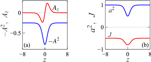
Figure 2: (a) The real (blue) and imaginary (red) part of the PT-symmetric Wadati potential generated by the base function (31). (b) The corresponding nonlinear mode (32b). Shown is the condensate density $a^{2}$ and the superfluid current $J=a^{2}\theta_{z}$. In these plots, $\alpha=\pi/4$ and $\varphi=\pi/3$.

7 Concluding remarks

Due to their unique properties, Gross-Pitaevskii equations with the Wadati potentials are of particular interest in PT-symmetric theories. Accordingly, it would be desirable to have a sufficiently diverse and ample collection of exactly-solvable Wadati potentials — these would serve as testing grounds for realistic physical models and starting points for perturbation expansions. The purpose of this contribution was to show how one can generate broad classes of PT-symmetric Wadati potentials along with exact localised solutions of the associated Gross-Pitaevskii equations.

The crux of our method lies in the ability to write the nonlinear second-order equation with a Wadati potential, as a symmetric system of two first-order equations. The potential function of this first-order system is nothing but the base function of the Wadati potential of the original second-order equation.

A practically-minded reader may naturally wonder what is the advantage of our approach over a simple reverse engineering, where the potential $V(x)$ is reconstructed from a postulated localised solution of equation (4):

$$V(x)=\frac{\psi_{xx}}{\psi}+g|\psi|^{2}-\kappa^{2}.$$ (33)

The answer is that the back-engineered potential (33) will generally not be of the Wadati variety.

In contrast, our method constructs the base function first. Only after the base $W(x)$ has been constructed does one proceed to form the potential $V=-W^{2}+iW_{x}$. Thus the resultant potential is Wadati by construction.

We have exemplified this procedure by constructing several exactly solvable PT-symmetric Wadati potentials for the attractive and repulsive Gross-Pitaevskii. In the case of the attractive (“focussing”) cubic nonlinearity, equation (15) reproduces the base function known in literature while the rational potential (17) is new. In the repulsive (“defocussing”) situation, the bases (28) and (30) constitute a continuous family of Wadati potentials supporting solitons over a nonvanishing background (lumps and bubbles). To the best of our knowledge, these potential-solution pairs are also new. Finally, we have constructed an exactly-solvable PT-symmetric potential supporting bubble-like solitons in a stationary flow of the superfluid. The corresponding potential base function is in (31).

- (1) J Muga, J Palao, B Navarro, and I Egusquiza, 2004 Complex absorbing potentials. Phys. Rep. 395, 357.
- (2) N Moiseyev, Non-Hermitian quantum mechanics (Cambridge: Cambridge University Press, 2009).
- (3) D Dast, D Haag, and H Cartarius, 2013 Eigenvalue structure of a Bose-Einstein condensate in a PT -symmetric double well, J. Phys. A 46, 375301
- (4) H Cartarius and G Wunner 2012 Model of a PT-symmetric Bose-Einstein condensate in a -function double-well potential. Phys. Rev. A, 86, 013612
- (5) C M Bender, 2007. Making sense of non-Hermitian Hamiltonians. Rep. Prog. Phys. 70, 947.
- (6) Z H Musslimani, K G Makris, R El-Ganainy, and D N Christodoulides 2008, Optical Solitons in PT Periodic Potentials. Phys. Rev. Lett. 100, 030402
- (7) A Ruschhaupt, F Delgado, and J G Muga 2005, Physical realization of PT-symmetric potential scattering in a planar slab waveguide. J Phys A: Math Gen 38, L171.
- (8) Z H Musslimani, K G Makris, R El-Ganainy and D N Christodoulides, 2008, Analytical solutions to a class of nonlinear Schrödinger equations with PT-like potentials. J. Phys. A: Math. Theor. 41, 244019
- (9) F Kh Abdullaev, V V Konotop, M Salerno and A V Yulin, 2010, Dissipative periodic waves, solitons, and breathers of the nonlinear Schrödinger equation with complex potentials. Phys. Rev. E 82, 056606
- (10) Z Shi, X Jiang, X Zhu, and H Li, 2011, Bright spatial solitons in defocusing Kerr media with PT-symmetric potentials. Phys. Rev. A 84, 053855
- (11) B Midya, and R Roychoudhury, 2013, Nonlinear localized modes in PT-symmetric Rosen-Morse potential wells. Phys. Rev. A 87, 045803
- (12) B Midya, 2015 Analytical stable Gaussian soliton supported by a parity-time symmetric potential with power-law nonlinearity. Nonlinear Dyn. 79, 409.
- (13) M Wadati, 2008. Construction of parity-time symmetric potential through the soliton theory. J Phys Soc Jpn 77, 074005.
- (14) A B Balantekin, J E Seger and S H Fricke, 1991. Dynamical effects in pair production by electric fields. Int J Mod Phys A 6, 695
- (15) R G Unanyan, 1992. Supersymmetry of a two-level system in a variable external field. Sov. Phys. JETP 74, 781
- (16) J F Beacom, A B Balantekin, 2007. A semiclassical approach to level crossing in supersymmetric quantum mechanics, in Supersymmetry and Integrable Models, Vol. 502 of the series Lecture Notes in Physics (Springer) p 296
- (17) A B Balantekin, 1998. Exact solutions for matter-enhanced neutrino oscillations, Phys. Rev. D 58, 013001
- (18) M Wadati and T Kamijo, 1974. On the extension of inverse scattering method. Prog Theor Phys 52, 397
- (19) A A Andrianov, M V Ioffe, F Cannata, and J P Dedonder, 1999. SUSY quantum mechanics with complex superpotentials and real energy spectra. Int J Mod Phys A 14, 2675
- (20) G L Lamb, 1980. Elements of Soliton Theory (Wiley). See section 2.12.
- (21) M Klaus and J K Shaw, 2002. Purely imaginary eigenvalues of Zakharov-Shabat systems. Phys. Rev. E 65, 036607
- (22) E N Tsoy, I M Allayarov, and F Kh Abdullaev, 2014. Stable localized modes in asymmetric waveguides with gain and loss. Opt Lett 39, 4215
- (23) M Wadati and K Ohkuma, 1982. Multiple-pole solutions of the modified Korteweg-de Vries equation. J Phys Soc Jpn 51, 2029
- (24) J Yang, 2014. Symmetry breaking of solitons in one-dimensional parity-time-symmetric optical potentials. Opt Lett 39, 5547
- (25) V V Konotop and D A Zezyulin, 2014. Families of stationary modes in complex potentials. Opt Lett 39, 5535
- (26) N Akhmediev, and A Ankiewicz (Editors), 2005. Dissipative Solitons (Springer, Berlin)
- (27) K G Makris, Z H Musslimani, D N Christodoulides, and S Rotter, 2015. Constant-intensity waves and their modulation instability in non-Hermitian potentials. Nat Commun 6, 7257
- (28) I V Barashenkov and V G Makhankov, 1988. Soliton-like “bubbles” in the system of interacting bosons. Phys Lett A 128, 52
- (29) I V Barashenkov and E Yu Panova, 1993. Stability and evolution of the quiescent and travelling solitonic bubbles. Physics D 69, 114