Multi-Contrast MRI Reconstruction with Structure-Guided Total Variation††thanks: This research was funded by the EPSRC grants EP/H0464110/1 and EP/K009745/1 and the UCL Department of Computer Science.
Abstract
Magnetic resonance imaging (MRI) is a versatile imaging technique that allows different contrasts depending on the acquisition parameters. Many clinical imaging studies acquire MRI data for more than one of these contrasts—such as for instance and weighted images—which makes the overall scanning procedure very time consuming. As all of these images show the same underlying anatomy one can try to omit unnecessary measurements by taking the similarity into account during reconstruction. We will discuss two modifications of total variation—based on i) location and ii) direction—that take structural a priori knowledge into account and reduce to total variation in the degenerate case when no structural knowledge is available. We solve the resulting convex minimization problem with the alternating direction method of multipliers that separates the forward operator from the prior. For both priors the corresponding proximal operator can be implemented as an extension of the fast gradient projection method on the dual problem for total variation. We tested the priors on six data sets that are based on phantoms and real MRI images. In all test cases exploiting the structural information from the other contrast yields better results than separate reconstruction with total variation in terms of standard metrics like peak signal-to-noise ratio and structural similarity index. Furthermore, we found that exploiting the two dimensional directional information results in images with well defined edges, superior to those reconstructed solely using a priori information about the edge location.
keywords: total variation, magnetic resonance imaging, MRI, a priori information, image reconstruction, regularization, structural similarity
AMS: 47A52, 49M30, 65J22, 94A08
1 Introduction
1.1 Multi-Contrast Magnetic Resonance Imaging
Magnetic resonance imaging (MRI) is a well established imaging modality with numerous applications. One of its key advantages is versatility: depending on image acquisition protocol, images with very different contrast and informational content can be acquired [36, 41]. Most common are images that are weighted by the relaxation times and but many more options are available. In clinical applications, often not one but several MRI images with different contrasts are acquired during one session. As an example, the UK Biobank111http://biobank.ctsu.ox.ac.uk/crystal/label.cgi, accessed August 14, 2015 contains for each subject MRI data for images weighted not only by and but also for images that are fluid-suppressed (FLAIR), or show susceptibility, diffusion or function. All of these data have to be acquired sequentially one at a time, which makes the whole scanning procedure rather lengthy. Therefore, shortening the acquisition time would not only reduce patient’s discomfort but would increase the patient throughput leading to more efficient use of the scanning facilities.
1.2 Magnetic Resonance Imaging and Compressed Sensing
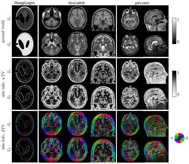
To speed up the scanning procedure, it has been proposed almost a decade ago to apply compressed sensing [11, 12, 16, 22] to MRI [38] which is still an active research topic [13, 37, 31, 45, 8, 14, 39, 29, 53, 49, 48]. One of the main ideas of compressed sensing is to acquire fewer measurements and to solve the reconstruction problem by exploiting a priori knowledge about the solution. Initially, the a priori knowledge has been sparsity in a wavelet basis and penalizing large total variations; the latter being related to sparsity of the image gradient. Over the years many other forms of a priori knowledge have been proposed for MRI reconstruction such as higher order total variation [31], sparsity in a self-learned dictionary [45] or regularization of dynamic sequences with the nuclear norm [37, 49] to name just a few. In a multi-contrast MRI scan, the images have very different information content, but as they are acquired from the same patient anatomy we know a priori that they are likely to show very similar structures [8, 29]. An example of a and weighted pair of MRI images of the same subject is shown on the right in figure 1. Parallel MRI [44, 28, 33, 50] is another example of image reconstruction problem which can benefit from exploiting common information. In [14] joint reconstruction of different coil images is performed in the framework of compressed sensing.
1.3 Contributions
In this paper we aim to exploit the expected redundancy in a series of multi-contrast MRI images by extracting information about i) the location of edges and ii) the direction of edges from one contrast to aid the reconstruction of the other. We propose two priors that enable us to incorporate a priori structural knowledge into a total variation functional. In both cases the prior is convex such that we can use algorithms from convex optimization to solve the minimization problem. A double-split allows us to apply the alternating direction method of multipliers (ADMM) where all but one update are in closed-form. An extension of the fast gradient projection method first proposed for the standard total variation in [6] is used to efficiently compute proximal operator for both priors.
1.4 Related Work
In this work we propose extensions of total variation, based on i) location and ii) direction, that can exploit structural a-priori knowledge and apply it to the multi-contrast MRI setting where structural information is available from another contrast. In this context we group the related work into the four following classes:
Total Variation with Local Weighting
Extensions of total variation or similar edge-preserving priors with spatially varying regularization parameter have been used before for optical tomography [2] and image denoising [26, 32]. While the weights are a priori defined by side information in [2], they are estimated based on local statistics in [26, 32]. In that respect this contribution improves upon [2] as our algorithm can handle a non-smooth formulation of the prior.
Total Variation and Directional Information
It has been proposed to include directional information into the total variation functional either by rotating the coordinate system and using locally the -norm [7] or by scaling preferred directions and applying the -norm [27, 4, 23, 35]. The directions are globally constant and predefined in [4] and based on the image content in [7, 27, 23, 35]. Our approach for directional information in the total variation functional shares similarities with [27, 23, 35]. While [27, 23, 35] compute the directions and scaling from the structure tensor of the current image estimate or the noisy input image, we project the gradient in the total variation functional onto a predefined vector field given by the other contrast.
One-Sided Reconstruction
Incorporating structural information by a prior has been used in other settings such as combined positron emission tomography (PET) with computed tomography or MRI [34, 9, 52], optical tomography [2], remote sensing [43, 24] or electric impedance tomography [30] but to the best of our knowledge has not been applied to multi-contrast MRI. In addition, only [2] and [30] share similarities with our approach. In [2] the authors propose to locally adapt the weight of the prior isotropically and used a smoothed penalty function to facilitate diffusion techniques for reconstruction. On the other hand while the prior in [30] is anisotropic, as it directionally dependent, it reduces to a quadratic prior when no edge information is available. In contrast, the here proposed priors reduce to total variation in absence of additional information.
Parallel Level Sets
The directional extension of total variation is related to the idea of measuring the difference in structure of two images by means of parallel level sets. A symmetric version of the latter has been used for joint reconstruction of PET-MRI [21, 20] and colour image processing [19]. We will point out the similarities and differences in more detail in §3. Moreover, in all [19, 21, 20] the parallel level sets functional has been smoothed and the problem has been solved using gradient based optimization. In contrast, here we consider the non-smooth convex formulation and propose a convex optimization algorithm for its solution.
2 Problem Setting and Notation
Our derivation is carried out in a fully discrete setting where the object of interest is sampled from a planar / volumetric MRI image. We will use this notation independently of the contrast, i.e. might represent a or weighted image. Moreover, we follow a standard assumption for many acquisition sequences of no or negligibly small phase so that we are effectively dealing with real-valued images. An extension to complex-valued images could be done by means of a non-linear forward operator [25, 56, 18] but this is out of scope of the present paper. Without phase, it is natural to assume that the MRI image is non-negative which we will incorporate into the reconstruction. With the common assumption of additive Gaussian noise [42, 40] a maximum a posteriori reconstruction with the prior proportional to , with functional to be defined later, is equivalent to the minimization problem
| (1) |
where is the MRI forward operator and the acquired data. Throughout the paper we use to denote the standard norm for complex vectors with being the Hermitian (complex conjugate transpose) of .
2.1 Forward Operator for Magnetic Resonance Imaging
The forward model in MRI is commonly assumed to be the Fourier transform [36]. As we model our image to be real-valued but the Fourier transform acts on complex images, we embed the real into the complex space by means of an operator . It is not difficult to show that is the adjoint of the real part restriction operator when we equip the complex space with the inner product . Moreover, let defining a sequence of sample locations which mimics an arbitrary MRI acquisition protocol. Then we can define a general sampling operator
| (2) |
where for better readability we denote the th component of the vector by . Here, we focus on the case of practical interest, , where the number of measurements is much smaller than the number of unknowns. With such defined operators, the MRI forward operator for our model can be expressed as their concatenation
| (3) |
Due to the embedding and the sampling this operator is in general not invertible.
2.2 Discrete Gradient
The functional in (1) encodes the a priori information in a way such that unlikely or undesirable solutions result in a large value . For images it is common to penalize changes between neighbouring pixel values which can be expressed by the discrete gradient operator.
At every location we define a discrete gradient . In the numerical simulations, we will use forward differences in two dimensions such that but other choices are possible, too. In general, the discrete gradient operator should be a linear mapping from space of images to the space of gradients. We make use of the discrete divergence operator defined as the negative adjoint of the gradient, i.e. for all it holds . For an approximation of the gradient with forward differences the matching approximation for the divergence corresponds to backward differences [3]. Moreover, let be the space of linear mappings from to . Then, we define the multiplication of a matrix-field with a vector-field pointwise as with , a matrix-vector multiplication at the particular location.
3 Modelling A Priori Information
3.1 Total Variation
A popular regularization in a variational formulation (1) is the total variation [47] which in our discrete setting reads
| (5) |
with the discrete gradient operator as defined in the previous section. The total variation has many desirable properties: it is convex and it leads to edge-preserved denoising. However, the standard formulation does not allow to incorporate any extra a priory knowledge about the solution.
3.2 Incorporating Structural Knowledge
3.2.1 A Priori Information on Location of Edges
While the actual intensities of two MRI contrasts are very different, their structure in terms of edges is likely to be highly correlated. To incorporate the information about the location of edges extracted from one contrast, , into the reconstruction of the other we propose to introduce weights into the total variation functional.
Definition 1 (Weighted Total Variation)
Let be a vector of weights. We define the weighted total variation as
| (6) |
Remark 2
An option for the choice of such weights is , where for some parameter . This choice results in , with the upper bound attained when there is no side information, i.e. , hence and the lower bound approached asymptotically for . The parameter controls what magnitude of an edge is considered to be ‘large’ and what is considered to be ‘small’. While in general this parameter could be a spatial map, for simplicity here we assume that it is constant over space.
Remark 3
Obviously, for the choice of uninformative weights, i.e. for all , the weighted total variation functional reduces to the standard total variation (5). Furthermore, implies that for all it holds .
3.2.2 A Priori Information on Direction of Edges
In the weighted total variation functional (6) we made use of the location of the edges by means of weights depending on the modulus of the gradient of the side information. However, it is reasonable to assume that these images do not only share the location but also the direction of edges modulo their sign. The latter is necessary as the actual intensity values are independent of one another such that in one image their might be a jump ‘up’ while in the other one there is a jump ‘down’.
Definition 4 (Directional Total Variation)
Let with be a vector-field and , i.e. . We call
| (7) |
the directional total variation.
Remark 5
In this paper we choose which captures the ‘structure’ of with more degrees of freedom than in the case of weighted total variation, cf. figure 1. As in the previous case, we will make use of an edge parameter that is related to the size of an edge. Similar to (6), we have with the lower bound being attained for and the upper bound approached as . In the limit , becomes the orthogonal projection onto the orthogonal complement of . Thus, in contrast to isotropic weighting of in (6), in the limit (7) penalizes only the component of that is orthogonal to resulting in an anisotropic weighting.
Remark 6
The directional total variation (7) for is related to the parallel level sets approach [19, 20, 18]. To be more precise, it was proven in [18] that
| (8) |
which shows that directional total variation is a special case of asymmetric parallel level sets with a different normalization of the side information . From (8) it can be seen that directional total variation favours parallel level sets. Indeed, on the one hand, (8) is minimal if and only if is parallel to (in the span of) and hence parallel to . On the other hand, as gradients are orthogonal to level sets, parallel gradients imply parallel level sets.
3.2.3 General Framework
Both functionals (6) and (7) can be uniformly written as
| (9) |
where the matrix-field depends on the structural knowledge derived from the image . In the case of weighted total variation,
| (10) |
the matrix-field is isotropic, i.e. it is directionally independent. On the other hand, for directional total variation,
| (11) |
the matrix field is anisotropic as it has principle directions along and orthogonal to . As was defined to be the normalized gradient field of these directions correspond to the normal and tangential direction to the level sets of .
4 Algorithmic Approach
In order to numerically solve problem (1) we will reformulate the problem such that it can be efficiently solved with the alternating direction method of multipliers (ADMM), see [1, 10] and references therein. As we model MRI images to be real-valued, it is efficient to perform two splits. Similar to total variation regularization, no closed-form proximal operator for priors of the form (9) exists, thus we revert to a variant of fast gradient projection algorithm [6].
4.1 Proximal Operator with Fast Gradient Projection
| regularization parameter | |
| proximal point | |
| number of iterations | |
| anisotropy (default = ) | |
| projection onto the set (default = ) | |
| initial dual variable (default = 0) |
| approximation of minimizer (primal variable) | |
| dual variable |
Evaluation of proximal operator for structural total variation (9), entails solution of the following convex minimization problem
| (12) |
with the non-empty, closed and convex constraint set . Although we are primarily interested in non-negativity constraints, i.e. , there is no need to be too specific at this point. Analogously to the case for usual total variation [6], structural total variation can be dualized as
| (13) |
where the supremum is taken over the unit ball in the gradient space . Substituting (13) into (12) and exchanging the order of the minimum and supremum as the function is convex in and concave in (see e.g. [46], Corollary 37.3.2) we obtain
| (14) | ||||
| (15) |
where the inner minimization in (14) has the solution . Following [6], the function under supremization in (15) can be equivalently rewritten as
| (16) |
and its gradient with respect to is given by
| (17) |
A variant of the fast projected gradient algorithm (with Nesterov acceleration) for solution of (15) and hence (12) is outlined in algorithm 1, where the orthogonal projection onto is given by
| (18) |
Remark 7
As an instance of fast iterative soft thresholding algorithm (FISTA), algorithm 1 with a step size converges in objective function values with rate [5] as is an upper bound on the Lipschitz constant of the gradient of the dual problem (17), see [6] for details. For both regularizers in this paper it holds . Moreover, we approximate the gradient with forward and the divergence with backward differences for which we have in 2D space [6] such that in both cases of interest is sufficient to guarantee convergence in function values.
4.2 Double-Split Alternating Direction Method of Multipliers
Recall that we want to solve (1)
with as in (9). To fully exploit the structure of our forward operator , we recast the problem as a constraint optimization problem
| (19) |
with the associated augmented Lagrangian
| (20) |
and are the scaled Lagrange multipliers. In order to make the algorithm as efficient as possible, and are associated with the first and with the second block of ADMM [1, 10]. Thus in every iteration we need to solve
| (21) |
| MRI data | |
| regularization parameter | |
| sampling | |
| number of iterations |
| approximate minimizer |
As the first minimization problem decouples in and , we obtain three update steps for ADMM, the first two of which can be performed in parallel
| (22) | |||
| (23) | |||
| (24) |
In (23) we used that for real . It should be noted that both and are diagonal matrices, so that the matrix inversion in (23), , reduces to a component-wise scaling and is therefore computationally efficient. The final ADMM algorithm can be found in 2. In each iteration of the algorithm, we apply once the discrete Fourier transform and its inverse as well as the proximal operator via algorithm 1. After each iteration, if the primal and dual residual are too far apart, we adjust the parameter according to the guidelines in [10].
Remark 8
In vector notation, the double split can be written as where has full column rank. If the we compute the proximal operator with sufficient accuracy, i.e. the errors are absolutely summable, and is constant, then algorithm 2 converges to a solution of (1) [17]. Numerically, we observe convergence for both and .
5 Numerical Experiments
5.1 Technical Details
5.1.1 Data and Algorithms
We numerically test the two extensions for total variation to incorporate structural information with six datasets that are either based on the Shepp-Logan phantom, realistically simulated MRI from BrainWeb [15] and clinical MRI images from a patient, cf. figure 1. We simulate the MRI data by sampling from the discrete Fourier transform in a variety of ways including Cartesian sampling (equidistantly and randomly undersampled), radial sampling (equidistantly spaced radial spokes, golden angle [55]) and spiral sampling (variable density and phyllotaxis [51]). In all cases we added Gaussian noise to the complex-valued MRI data with standard deviation scaled such that for fully sampled data the expected -norm of the noise is 5% of the -norm of the noise-free data.
Both algorithms 1 and 2 have been implemented in MATLAB R2015a. The algorithms and the datasets used in this paper are available as supplementary material.
5.1.2 Quality Measures and Parameter Selection
We evaluate the results in terms of the peak signal-to-noise (PSNR) and the structural similarity index (SSIM) [54] both available in the image processing toolbox in MATLAB R2015a.
The regularization parameter and the edge parameter are chosen to maximize the SSIM between the reconstructed result and the ground truth.
5.2 Results
5.2.1 Parameter Estimation
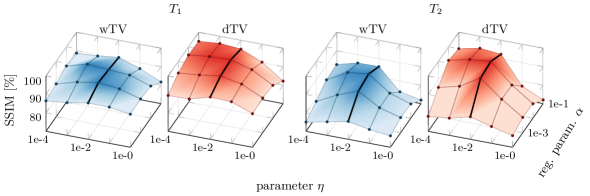
Both proposed extensions of total variation have a parameter that relates to the magnitude of the gradients in the side information. Figure 2 shows the SSIM of the reconstructions of and weighted images from radially sampled BrainWebA data using both structure enhancing regularizers in dependence of the regularization parameter and the edge parameter . In all cases the best results are obtained for = 1e-2 which corresponds to approximately 1% of the maximal gradient magnitude. For a large value of —in this example approximately 1—both regularizers perform the same and both coincide with total variation (not shown). Similar plots were obtained for the other data sets and sampling patterns and hence will be omitted for brevity. In what follows the edge parameter is always chosen to be 1e-2.
5.2.2 Visual Assessment
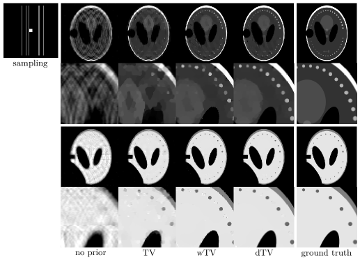
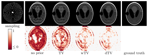
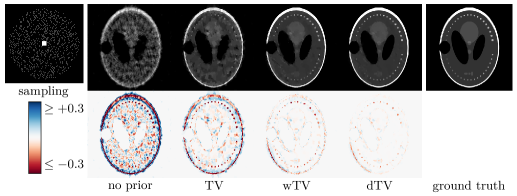
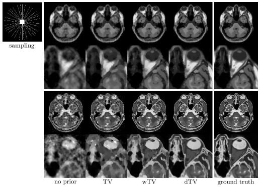
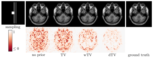
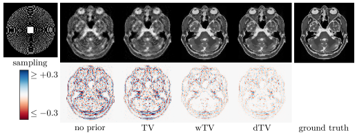
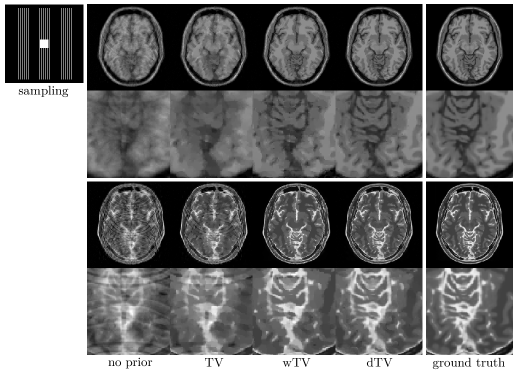
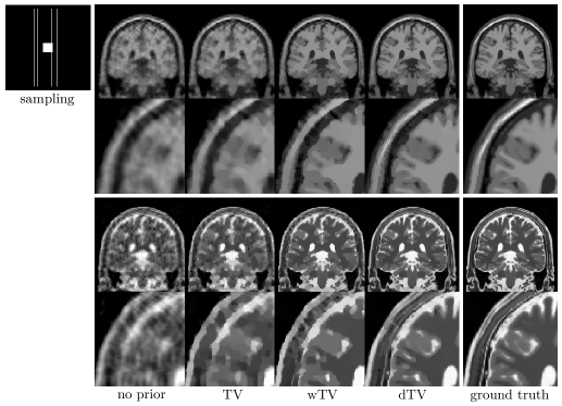
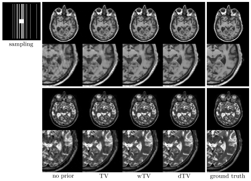
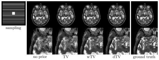
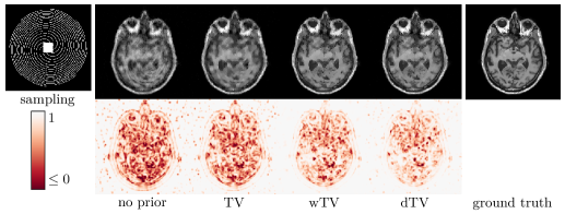
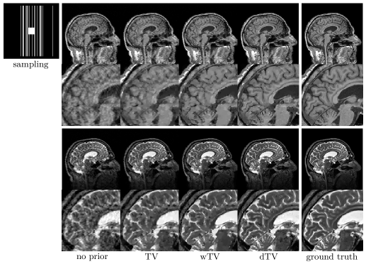
Figures 5 - 14 show results of reconstructions of and weighted images of the six ground truth image sets depicted in figure 1 using different sampling schemes. Whenever appropriate we include close-ups or SSIM maps and difference images to aid quantitative comparison. While most of the images speak for themselves and some observations are included in the captions we would like to make some general comments. In all of the aforementioned figures, but probably most visibly in figure 10, incorporating structural knowledge from the other contrast does visually improve the reconstruction using either or . When comparing and , one notices that while results in patchy images, is able to recover smooth structures accurately. Moreover, including the directional information yields another level of improvement of fine details.
5.2.3 Quantitative Assessment
Quantitative analysis of the results is summarized in figures 5.2.3 and 5.2.3, and table 5.2.3. Figure 5.2.3 shows the reconstruction quality for all six test cases in dependence of the regularization parameter. Whenever more than one sampling scheme was used, the solid line corresponds to the mean performance with the worst and best performance indicated by shaded lines. For all test cases, but especially for -weighted SheppLogan and BrainWeb, and strongly outperforms the standard total variation. Moreover, the curves are layered which means that the results are not only better for one choice of regularization parameter but for all choices shown.
Figure 5.2.3 shows the performance for the optimal value of the regularization parameter for all test cases (data sets and sampling schemes). Also here, the curves are layered, meaning that in every test case outperforms all the other methods. The average performance can be read out from table 5.2.3, where again consistently performs best with respect to all measures. The particular differences in performance between the methods vary strongly between the data sets, chosen samplings and contrasts but on average improves on total variation by about 6dB in PSNR and 8% in SSIM for both contrasts, cf. table 5.2.3.
| no prior | no prior | ||||||||
|---|---|---|---|---|---|---|---|---|---|
| PSNR [dB] | min | 18.7 | 22.6 | 25.8 | 26.0 | 21.4 | 21.8 | 24.6 | 27.0 |
| max | 29.4 | 29.9 | 32.3 | 38.0 | 26.6 | 33.0 | 34.7 | 39.0 | |
| mean | 25.2 | 26.9 | 29.4 | 32.7 | 23.2 | 26.1 | 28.5 | 32.6 | |
| median | 26.4 | 27.3 | 29.8 | 33.8 | 23.0 | 24.8 | 27.1 | 30.6 | |
| SSIM [%] | min | 63.7 | 81.3 | 89.7 | 90.7 | 74.6 | 79.2 | 89.3 | 91.7 |
| max | 92.3 | 94.7 | 95.3 | 98.9 | 90.2 | 98.0 | 97.8 | 99.2 | |
| mean | 81.9 | 87.8 | 93.1 | 96.2 | 80.2 | 87.9 | 93.3 | 96.6 | |
| median | 86.6 | 88.2 | 93.5 | 96.7 | 79.1 | 85.8 | 92.5 | 96.9 | |
![[Uncaptioned image]](/html/1511.06631/assets/x15.png)
![[Uncaptioned image]](/html/1511.06631/assets/x16.png)
5.3 Discussion
The largest improvements were obtained for the -weighted SheppLoganand both contrasts from BrainWeb. We attribute this to the higher level of detail in than in version of SheppLogan, which in turn results in having higher total variation than . While the quantitative results for patient do not indicate much improvement, visual inspection corroborates the increase in image quality. This might be due to the fact that the noisy reconstructed MRI images have been taken as ground truth and in this case the similarity measure do not match human perception.
6 Conclusions
In this paper we extended total variation to accommodate the structural a priori information available from another contrast in MRI. The structural information can be either purely on the location or on the location and direction of edges. In both cases, the prior is convex so that we can use efficient methods from convex optimization to solve the problem. The numerical results with numerous test cases show that exploiting structural information is beneficial in the reconstruction of highly undersampled MRI. Moreover, utilizing directional information yields not only better defined images but also better reconstruction of smooth structures and fine details.
In the future, we will extend the proposed framework to more than a pair of contrasts and so to exploit the structural similarity of a whole sequence of MRI images. Moreover, we intend to extend our method to joint reconstruction of multiple contrasts.
Acknowledgements
The authors would like to thank Felix Lucka and Ivana Drobnjak for helpful discussions. Moreover, we highly appreciate the help of Ninon Burgos and Jonathan Schott who provided the real MRI images.
References
- [1] Manya V Afonso, José M Bioucas-Dias and Mário A T Figueiredo “Fast Image Recovery using Variable Splitting and Constrained Optimization” In IEEE Transactions on Image Processing 19.9, 2010, pp. 2345–2356 DOI: 10.1109/TIP.2010.2047910
- [2] Simon R Arridge, Ville Kolehmainen and Martin J Schweiger “Reconstruction and Regularisation in Optical Tomography” In Interdisciplinary Workshop on Mathematical Methods in Biomedical Imaging and Intensity-Modulated Radiation, 2007
- [3] G. Aubert and P. Kornprobst “Mathematical Problems in Image Processing: Partial Differential Equations and the Calculus of Variations”, Applied Mathematical Sciences Springer, 2001
- [4] Ilker Bayram and Mustafa E. Kamasak “A Directional Total Variation” In IEEE Signal Processing Letters 19.12, 2012, pp. 265–269 DOI: 10.1109/LSP.2012.2220349
- [5] Amir Beck and Marc Teboulle “A Fast Iterative Shrinkage-Thresholding Algorithm for Linear Inverse Problems” In SIAM Journal on Imaging Sciences 2.1, 2009, pp. 183–202 DOI: 10.1137/080716542
- [6] Amir Beck and Marc Teboulle “Fast Gradient-Based Algorithms for Constrained Total Variation Image Denoising and Deblurring Problems” In IEEE Transactions on Image Processing 18.11, 2009, pp. 2419–2434 DOI: 10.1109/TIP.2009.2028250
- [7] Benjamin Berkels, Martin Burger, Marc Droske, Oliver Nemitz and Martin Rumpf “Cartoon Extraction Based on Anisotropic Image Classification” In Vision, Modeling, and Visualization Proceedings, 2006, pp. 293–300
- [8] Berkin Bilgic, Vivek K Goyal and Elfar Adalsteinsson “Multi-Contrast Reconstruction with Bayesian Compressed Sensing” In Magnetic Resonance in Medicine 66.6, 2011, pp. 1601–15 DOI: 10.1002/mrm.22956
- [9] James E Bowsher et al. “Utilizing MRI Information to Estimate F18-FDG Distributions in Rat Flank Tumors” In IEEE Nuclear Science Symposium and Medical Imaging Conference, 2004, pp. 2488–2492 DOI: 10.1109/NSSMIC.2004.1462760
- [10] Stephen Boyd “Distributed Optimization and Statistical Learning via the Alternating Direction Method of Multipliers” In Foundations and Trends® in Machine Learning 3.1, 2010, pp. 1–122 DOI: 10.1561/2200000016
- [11] Emmanuel J Candès, Justin K Romberg and Terence Tao “Robust Uncertainty Principles: Exact Signal Reconstruction From Highly Incomplete Frequency Information” In IEEE Transactions on Information Theory 52.2, 2006, pp. 489–509 DOI: 10.1109/TIT.2005.862083
- [12] Emmanuel J Candès, Justin K Romberg and Terence Tao “Stable Signal Recovery from Incomplete and Inaccurate Measurements” In Communications on Pure and Applied Mathematics LIX, 2006, pp. 1207–1223 DOI: 10.1002/cpa.20124
- [13] T.-C. Chang, L. He and T. Fang “MR Image Reconstruction from Sparse Radial Samples Using Bregman Iteration” In International Society for Magnetic Resonance in Medicine 4, 2006, pp. 696
- [14] Chen Chen, Yeqing Li and Junzhou Huang “Calibrationless Parallel MRI with Joint Total Variation Regularization” In Medical Image Computing and Computer-Assisted Intervention, 2013, pp. 106–114
- [15] Chris A Cocosco, Vasken Kollokian, Remi K.-S. Kwan, G Bruce Pike and Alan C Evans “BrainWeb: Online Interface to a 3D MRI Simulated Brain Database” In NeuroImage 5, 1997, pp. 425
- [16] David L Donoho “Compressed Sensing” In IEEE Transactions on Information Theory 52.4, 2006, pp. 1289–1306 DOI: 10.1109/TIT.2006.871582
- [17] Jonathan Eckstein and Dimitri P. Bertsekas “On the Douglas-Rachford Splitting Method and the Proximal Point Algorithm for Maximal Monotone Operators” In Mathematical Programming 55.1-3, 1992, pp. 293–318 DOI: 10.1007/BF01581204
- [18] Matthias Joachim Ehrhardt “Joint Reconstruction for Multi-Modality Imaging with Common Structure”, 2015, pp. 1–177
- [19] Matthias Joachim Ehrhardt and Simon R Arridge “Vector-Valued Image Processing by Parallel Level Sets” In IEEE Transactions on Image Processing 23.1, 2014, pp. 9–18 DOI: 10.1109/TIP.2013.2277775
- [20] Matthias Joachim Ehrhardt, Kris Thielemans, Luis Pizarro, David Atkinson, Sébastien Ourselin, Brian F Hutton and Simon R Arridge “Joint Reconstruction of PET-MRI by exploiting Structural Similarity” In Inverse Problems 31 IOP Publishing, 2015, pp. 015001 DOI: 10.1088/0266-5611/31/1/015001
- [21] Matthias Joachim Ehrhardt, Kris Thielemans, Luis Pizarro, Pawel Markiewicz, David Atkinson, Sébastien Ourselin, Brian F Hutton and Simon R Arridge “Joint Reconstruction of PET-MRI by Parallel Level Sets” In IEEE Nuclear Science Symposium and Medical Imaging Conference, 2014
- [22] Yonina C Eldar and Gitta Kutyniok “Compressed Sensing: Theory and Applications” Cambridge University Press, 2012
- [23] Virginia Estellers, Stefano Soatto and Xavier Bresson “Adaptive Regularization With the Structure Tensor” In IEEE Transactions on Image Processing 24.6, 2015, pp. 1777–1790
- [24] Faming Fang, Fang Li, Chaomin Shen and Guixu Zhang “A Variational Approach for Pan-Sharpening” In IEEE Transactions on Image Processing 22.7, 2013, pp. 2822–2834 DOI: 10.1109/TIP.2013.2258355
- [25] Jeffrey A Fessler and Douglas C Noll “Iterative Image Reconstruction in MRI with Separate Magnitude and Phase Regularization” In International Symposium on Biomedical Imaging, 2004, pp. 209–212
- [26] Markus Grasmair “Locally Adaptive Total Variation Regularization” In SSVM 2009 5567 LNCS, 2009, pp. 331–342 DOI: 10.1007/978-3-642-02256-2\_28
- [27] Markus Grasmair and Frank Lenzen “Anisotropic Total Variation Filtering” In Applied Mathematics & Optimization 62.3, 2010, pp. 323–339 DOI: 10.1007/s00245-010-9105-x
- [28] Mark A Griswold, Peter M Jakob, Robin M Heidemann, Mathias Nittka, Vladimir Jellus, Jianmin Wang, Berthold Kiefer and Axel Haase “Generalized Autocalibrating Partially Parallel Acquisitions (GRAPPA)” In Magnetic Resonance in Medicine 47, 2002, pp. 1202–1210 DOI: 10.1002/mrm.10171
- [29] Junzhou Huang, Chen Chen and Leon Axel “Fast Multi-Contrast MRI Reconstruction” In Magnetic Resonance Imaging 32.10 Elsevier Inc., 2014, pp. 1344–52 DOI: 10.1016/j.mri.2014.08.025
- [30] Jari P Kaipio, Ville Kolehmainen, Marko Vauhkonen and Erkki Somersalo “Inverse Problems with Structural Prior Information” In Inverse Problems 15.3, 1999, pp. 713–729 DOI: 10.1088/0266-5611/15/3/306
- [31] Florian Knoll, Kristian Bredies, Thomas Pock and Rudolf Stollberger “Second order total generalized variation (TGV) for MRI.” In Magnetic Resonance in Medicine 65.2, 2011, pp. 480–91 DOI: 10.1002/mrm.22595
- [32] Florian Knoll, Y. Dong, C. Langskammer, Michael Hintermüller and Rudolf Stollberger “Total Variation Denoising with Spatially Dependent Regularization” In Proc. Intl. Soc. Mag. Reson. Med. 18, 2010, pp. 5088
- [33] David J Larkman and Rita G Nunes “Parallel Magnetic Resonance Imaging” In Physics in Medicine and Biology 52.7, 2007, pp. R15–55 DOI: 10.1088/0031-9155/52/7/R01
- [34] Richard M. Leahy and X. Yan “Incorporation of Anatomical MR Data for Improved Functional Imaging with PET” In Information Processing in Medical Imaging, 1991, pp. 105–120 Springer DOI: 10.1007/BFb0033746
- [35] Frank Lenzen and Johannes Berger “Solution-Driven Adaptive Total Variation Regularization” In SSVM, 2015, pp. 203–215 DOI: 10.1007/978-3-642-24785-9
- [36] Zhi-Pei Liang and Paul C Lauterbur “Principles of Magnetic Resonance Imaging: A Signal Processing Perspective”, IEEE Press Series in Biomedical Engineering SPIE Optical Engineering Press, 2000
- [37] Sajan Goud Lingala, Yue Hu, Edward Dibella and Mathews Jacob “Accelerated Dynamic MRI Exploiting Sparsity and Low-Rank Structure: K-T SLR” In IEEE Transactions on Medical Imaging 30.5, 2011, pp. 1042–1054 DOI: 10.1109/TMI.2010.2100850
- [38] Michael Lustig, David L Donoho and John M. Pauly “Sparse MRI: The Application of Compressed Sensing for Rapid MR Imaging” In Magnetic Resonance in Medicine 58.6, 2007, pp. 1182–1195 DOI: 10.1002/mrm.21391
- [39] Dan Ma, Vikas Gulani, Nicole Seiberlich, Kecheng Liu, Jeffrey L Sunshine, Jeffrey L Duerk and Mark A Griswold “Magnetic Resonance Fingerprinting” In Nature 495.7440 Nature Publishing Group, 2013, pp. 187–92 DOI: 10.1038/nature11971
- [40] Albert Macovski “Noise in MRI” In Magnetic Resonance in Medicine 36.3 Wiley Online Library, 1996, pp. 494–497 DOI: 10.1002/mrm.1910360327
- [41] Donald W McRobbie, Elizabeth A Moore, Martin J Graves and Martin R Prince “MRI - From Picture to Proton” Cambridge University Press, 2006
- [42] E R McVeigh, R M Henkelman and M J Bronskill “Noise and Filtration in Magnetic Resonance Imaging” In Medical Physics 12.5, 1985, pp. 586–591 DOI: 10.1118/1.595679
- [43] Michael Möller, Todd Wittman, Andrea L. Bertozzi and Martin Burger “A Variational Approach for Sharpening High Dimensional Images” In SIAM Journal on Imaging Sciences 5.1, 2012, pp. 150–178 DOI: 10.1137/100810356
- [44] Klaas P Pruessmann, Markus Weiger, Markus B Scheidegger and Peter Boesiger “SENSE: Sensitivity Encoding for Fast MRI” In Magnetic Resonance in Medicine 42.5, 1999, pp. 952–62
- [45] Saiprasad Ravishankar and Yoram Bresler “MR Image Reconstruction From Highly Undersampled K-Space Data by Dictionary Learning” In IEEE Transactions on Medical Imaging 30.5, 2011, pp. 1028–41 DOI: 10.1109/TMI.2010.2090538
- [46] R T Rockafellar “Convex Analysis”, Princeton landmarks in mathematics and physics Princeton, New Jersey: Princeton University Press, 1970
- [47] Leonid I Rudin, Stanley Osher and Emad Fatemi “Nonlinear Total Variation based Noise Removal Algorithms” In Physica D: Nonlinear Phenomena 60.1 Elsevier, 1992, pp. 259–268 DOI: 10.1016/0167-2789(92)90242-F
- [48] Daniel K. Sodickson, Li Feng, Florian Knoll, Martijn Cloos, Noam Ben-Eliezer, Leon Axel, Hersh Chandarana, Tobias Block and Ricardo Otazo “The Rapid Imaging Renaissance: Sparser Samples, Denser Dimensions, and Glimmerings of a Grand Unified Tomography” In Proceedings of SPIE 9417, 2015, pp. 94170G1–14 DOI: 10.1117/12.2085033
- [49] Benjamin Trémoulhéac, Nikolaos Dikaios, David Atkinson and Simon R Arridge “Dynamic MR Image Reconstruction - Separation From Undersample (k-t)-Space via Low-Rank Plus Sparse Prior” In IEEE Transactions on Medical Imaging 33.8, 2014, pp. 1689–1701 DOI: 10.1109/TMI.2014.2321190
- [50] Martin Uecker, Peng Lai, Mark J. Murphy, Patrick Virtue, Michael Elad, John M. Pauly, Shreyas S. Vasanawala and Michael Lustig “ESPIRiT - An Eigenvalue Approach to Autocalibrating Parallel MRI: Where SENSE meets GRAPPA” In Magnetic Resonance in Medicine 71, 2014, pp. 990–1001 DOI: 10.1002/mrm.24751
- [51] Helmut Vogel “A Better Way to Construct the Sunflower Head” In Mathematical Biosciences 44, 1979, pp. 179–189
- [52] Kathleen Vunckx, Ameya Atre, Kristof Baete, Anthonin Reilhac, Christophe M Deroose, Koen Van Laere and Johan Nuyts “Evaluation of Three MRI-based Anatomical Priors for Quantitative PET Brain Imaging” In IEEE Transactions on Medical Imaging 31.3, 2012, pp. 599–612 DOI: 10.1109/TMI.2011.2173766
- [53] Qiu Wang, Michael Zenge, Hasan Ertan Cetingul, Edgar Mueller and Mariappan S Nadar “Novel Sampling Strategies for Sparse MR Image Reconstruction” In International Society for Magnetic Resonance in Medicine 55.3, 2014, pp. 4249
- [54] Zhou Wang, Alan Conrad Bovik, Hamid Rahim Sheikh and Eero P Simoncelli “Image Quality Assessment: From Error Visibility to Structural Similarity” In IEEE Transactions on Image Processing 13.4, 2004, pp. 600–12
- [55] Stefanie Winkelmann, Tobias Schaeffter, Thomas Koehler, Holger Eggers and Olaf Doessel “An Optimal Radial Profile Order based on the Golden Ratio for Time-Resolved MRI” In IEEE Transactions on Medical Imaging 26.1, 2007, pp. 68–76 DOI: 10.1109/TMI.2006.885337
- [56] Marcelo V W Zibetti and Alvaro Rodolfo De Pierro “Separate Magnitude and Phase Regularization in MRI with Incomplete Data: Preliminary Results” In International Symposium on Biomedical Imaging, 2010, pp. 736–739