LEAP: the large European array for pulsars

Abstract

The Large European Array for Pulsars (LEAP) is an experiment that harvests the collective power of Europe’s largest radio telescopes in order to increase the sensitivity of high-precision pulsar timing. As part of the ongoing effort of the European Pulsar Timing Array (EPTA), LEAP aims to go beyond the sensitivity threshold needed to deliver the first direct detection of gravitational waves. The five telescopes presently included in LEAP are: the Effelsberg telescope, the Lovell telescope at Jodrell Bank, the Nançay radio telescope, the Sardinia Radio Telescope and the Westerbork Synthesis Radio Telescope. Dual polarization, Nyquist-sampled time-series of the incoming radio waves are recorded and processed offline to form the coherent sum, resulting in a tied-array telescope with an effective aperture equivalent to a 195 -m diameter circular dish. All observations are performed using a bandwidth of 128 MHz centered at a frequency of 1396 MHz. In this paper, we present the design of the LEAP experiment, the instrumentation, the storage and transfer of data, and the processing hardware and software. In particular, we present the software pipeline that was designed to process the Nyquist-sampled time-series, measure the phase and time delays between each individual telescope and a reference telescope and apply these delays to form the tied-array coherent addition. The pipeline includes polarization calibration and interference mitigation. We also present the first results from LEAP and demonstrate the resulting increase in sensitivity, which leads to an improvement in the pulse arrival times.

1 Introduction

Fundamental physics and our understanding of the Universe are at an important crossroad. We can now compute the evolution of the Universe back in time until a small fraction of a second after the Big Bang, and the experimental evidence for our standard model of particle physics has been exemplified by the detection of the Higgs boson (Chatrchyan et al., 2012; Aad et al., 2012). At the centre of the theoretical understanding of both of these branches of physics are Einstein’s theory of general relativity (GR) and the laws of quantum mechanics. Both theories are extremely successful, having passed observational and experimental tests with flying colours (e.g. Kramer et al. 2006). Nevertheless, they seem to be incompatible, and attempts to formulate a new theory of quantum gravity, which would unite the classical world of gravitation with the intricacies of quantum mechanics, remain an important challenge. In this quest it is therefore hugely important to know whether GR is the right theory of gravity after all.

Because gravity is a rather weak force, it usually requires massive astronomical bodies to test the predictions of Einstein’s theory. One of these predictions involves the essential concept that space and time are combined to form space-time that is curved in the presence of mass. As masses move and accelerate, ripples in space-time are created that propagate through the Universe. These gravitational waves (GWs) are known to exist from the observed decay of the orbital period in compact systems of two orbiting stars as the GWs carry energy away (e.g. Taylor & Weisberg 1982; Kramer et al. 2006). After inferring their existence indirectly in this way, the next great challenge is the direct detection of GWs.

The frequency range for which we can expect GW emission from a variety of sources covers more than 20 orders of magnitude. Efforts to measure the displacement of masses on Earth as GWs pass through terrestrial laboratories are ongoing worldwide, with the operation and upgrade of detectors such as (Advanced) LIGO (Abbott et al., 2009), (Advanced) Virgo (Accadia et al., 2012) or GEO600 (Grote & LIGO Scientific Collaboration, 2010). These detectors probe GWs at kHz-frequencies and are therefore sensitive to signals from merging binary neutron stars or black hole systems. At slightly lower GW frequencies, a space-based interferometer like the proposed eLISA observatory will be sensitive to Galactic binaries and coalescing binary black holes with masses in the range of $10^{4}$ to $10^{6}$ M_⊙ (Amaro-Seoane et al., 2013).

To reach a much lower GW frequency range (complementary to the frequency range covered by ground-based detectors), we can use observations of radio pulsars. Radio pulsars are spinning neutron stars that emit beams of radio emission along their magnetic axes. The pulses of radiation detected by radio telescopes correspond to the passing of the narrow beam across the telescope with each rotation. The fact that these pulses arrive with such regularity, from the best pulsars, means that they act like cosmic clocks. In a Pulsar Timing Array (PTA) experiment, we can use these most stable pulsars, millisecond pulsars (MSPs), as the arms of a huge Galactic gravitational wave detector, to enable a direct detection of GWs (Detweiler, 1979; Hellings & Downs, 1983).

There are currently three major PTA experiments. In Australia, the Parkes Pulsar Timing Array (Manchester et al., 2013) is utilising the 64-m Parkes telescope. In North America, NANOGrav is making use of the 100-m Green Bank Telescope (GBT) and the 305-m Arecibo telescope (Demorest et al., 2013). In Europe, the largest number of large radio telescopes is available: the European Pulsar Timing Array (EPTA) has access to the 100-m Effelsberg telescope in Germany, the 76-m Lovell telescope at Jodrell Bank in the UK, the 94-m equivalent Westerbork Synthesis Telescope (WSRT) in the Netherlands, the 94-m equivalent Nançay Radio Telescope (NRT) in France and, as the latest addition, the 64-m Sardinia Radio Telescope (SRT) in Italy. For a recent summary of the details of the mode of operation of the EPTA, its source list and experimental achievements (e.g. the derived limits for the signal strength of a stochastic gravitational wave background or the energy scale of cosmic string networks) and major theoretical studies, we refer to Kramer & Champion (2013); Lentati et al. (2015); Desvignes et al. (submitted). All three experiments also work together within the International Pulsar Timing Array (IPTA, Hobbs et al. 2010; Manchester & IPTA 2013).

Despite the apparent simplicity of a PTA experiment, the timing precision required for the detection of GWs is very much at the limit of what is technically possible today. Indeed, all ongoing efforts summarised above currently fail to achieve the needed sensitivity (Demorest et al., 2013; Lentati et al., 2015; Shannon et al., 2013). As timing precision increases essentially with telescope sensitivity (up to a point where the changing interstellar medium along the line-of-sight and the intrinsic pulse jitter become dominant, e.g. Liu et al. 2011; Cordes & Shannon 2010), an increase in telescope sensitivity is needed. In the future, radio astronomers expect to operate a new radio telescope known as the Square-Kilometre-Array (SKA). The study of the low-frequency GW sky is one of the major SKA Key Science Projects (Janssen et al., 2014). The SKA sensitivity will be so large (ultimately up to two orders of magnitude higher than that of the largest steerable dishes) that GW studies may become routine and will open up an era of GW astronomy that will allow us to study the universe in a completely different way.

In this paper, we present the first comprehensive introduction to the Large European Array for Pulsars (LEAP), a new experiment that uses a novel method and observing mode to harvest the collective power of Europe’s largest radio telescopes in order to obtain a “leap” in the PTA sensitivity. The long-term aim for LEAP is to go beyond the sensitivity threshold needed to obtain the first direct detection of GWs. LEAP represents the next logical, intermediate step between the current state-of-the-art of pulsar timing and the sensitivities achievable with the SKA. The efforts and technical advances that LEAP brings (as described below) are essential steps towards the exploitation of the SKA and its study of the nHz-GW sky.

The LEAP experiment is introduced in §2; in §3 we describe the participating telescopes and the instruments; in §4 the pipelines involved in the calibration and analysis of the data are explained. The observing strategy is outlined in §5 and initial results are presented in §6. We conclude in §7.

2 Experimental design

The goal of the LEAP project is to enhance the sensitivity of pulsar timing observations by combining the signals of the five largest European radio telescopes. The combination of individual telescope signals can be done in two ways: coherently and incoherently. In the incoherent addition signals are added after detection (squaring of the signal) hence removing the phase information of the electromagnetic signal received by the individual telescopes, so that the signal-to-noise ratio (S/N) increases with the square-root of the number of added telescopes. By adapting proven techniques from existing Very Long Baseline Interferometry (VLBI) experiments (e.g. Thompson et al., 1991), the phase delays between the signals received at the individual telescopes can be determined and corrected for, allowing for the coherent addition of the signals (e.g. as described for LOFAR in Stappers et al. 2011). In this mode, the telescopes form a “tied array” beam that is pointed to a specific sky position (here that of a millisecond pulsar). In the standard operation mode described below, LEAP forms a single tied-array beam. In this case, the S/N of the LEAP observation is the (optimal) linear sum of the S/Ns of the individual telescopes.

Forming the coherent LEAP tied-array beam shares many similarities with a multi-element interferometer. In both cases, the individual telescopes observe the same source over an identical range of observing frequencies and correct the signals of the individual telescopes for (differences in) the delays due to geometry, atmosphere, instruments and clocks. In an interferometer, the correlated signals are ultimately used to form images with high spatial resolution, while for a tied-array, the signals from the individual telescopes are added coherently in phase to form the coherent sum. For short baselines of up to several kilometers, such as for multi-element interferometers like the Australian Telescope Compact Array (ATCA), the Jansky Very Large Array (JVLA), the Giant Metre Radio Telescope (GMRT), the Low Frequency Array (LOFAR) and the Westerbork Synthesis Radio Telescope (WSRT), these corrections can be applied in analog or digital hardware, or software, producing the tied-array signal in (or near) real-time (e.g. Karuppusamy et al. 2008; Roy et al. 2012). For longer baselines, it is usually required to store the digitized Nyquist-sampled time-series and process the data offline. This approach is used in imaging observations for long baseline interferometers such as global VLBI observations or usually that of the European VLBI Network. Recent progress with the new SFXC software correlator would allow the formation of a tied-array out of the telescopes participating in the European VLBI Network (Kettenis & Keimpema, 2014; Keimpema et al., 2015).

The LEAP project forms a tied-array telescope specifically designed to provide high S/N observations of the MSPs that are in the EPTA (see Table 2 in Kramer & Champion 2013, and also Desvignes et al. 2015). Due to the availability of sensitive L-band (1.4 GHz) receivers at all EPTA telescopes, LEAP observations are obtained at 1396 MHz with an overlapping bandwidth of 128 MHz. During monthly observing sessions, both pulsars and suitable phase calibrators are observed, and the data are recorded to disk. These disks are then shipped to Jodrell Bank Observatory, where the data are correlated (in order to determine the relative phase delays) and coherently added using software running on a high-performance computer cluster.

3 Telescopes and instruments

3.1 Telescopes

We describe here in more detail the telescopes presently involved in LEAP:

The 100-m telescope located in Effelsberg, Germany, is a fully-steerable parabolic dish with an altitude-azimuth mount, and is operated by the Max-Planck Institut für Radioastronomie. For LEAP observations, depending on scheduling constraints, one of the two L-band (1.4 GHz) receivers (multi-beam or single-pixel) is used. Both receivers provide signals corresponding to the two hands of circular polarization at their outputs. The receivers use cryogenically-cooled low noise amplifiers (LNAs) based on high electron mobility transistors (HEMT), resulting in a system temperature of 24 K. At L-band (1.4 GHz), the telescope has a gain of 1.5 K Jy^-1.

The 250-foot (76.2-m) Lovell telescope at Jodrell Bank Observatory has a parabolic surface with an altitude-azimuth mount. The telescope is operated by the Jodrell Bank Centre for Astrophysics at the University of Manchester. A cryogenically-cooled receiver that is placed at the primary focus and is capable of observing a 500 MHz wide band between 1.3 and 1.8 GHz with a system temperature of 25 K. This receiver has linear feeds, but uses a quarter-wave plate to produce two hands of circular polarization. The telescope gain for L-band (1.4 GHz) observations is 1 K Jy^-1 at 45^∘ of elevation.

The Nançay radio telescope is a transit telescope of the Krauss design, in which the radiation is reflected via a movable flat mirror onto a spherical mirror, and then received at a movable focus cabin. The telescope has an equivalent diameter of 94 m. Depending on the declination of the source, the telescope can track sources for approximately 1 hour. The L-band receiver covers the frequency range from 1.1 to 1.9 GHz with a system temperature of 35 K, and has a telescope gain of 1.4 K Jy^-1 at these frequencies.

The 64-m Sardinia Radio Telescope located in San Basilio, Sardinia, is a fully-steerable parabolic dish with an altitude-azimuth mount and a modern active surface that makes it one of the most technologically-advanced telescopes in the world. It is the newest addition to the LEAP project. The SRT joined LEAP in July 2013 during its scientific validation phase. LEAP observations are done using a cryogenically-cooled dual-band 1.4 GHz and 350 MHz confocal receiver at the primary focus of the telescope. The L-band receiver has a bandwidth of 500 MHz (ranging from 1.3 to 1.8 GHz), a system temperature of 20 K and has linear feeds. The corresponding telescope gain is 0.63 K Jy^-1.

The Westerbork Synthesis Radio Telescope is an interferometer used as a tied-array consisting of 14 equatorially-mounted, 25-m diameter, fully-steerable parabolic dishes (Baars & Hooghoudt, 1974). The telescopes are equipped with multi-frequency front-ends (MFFEs) that cover frequencies from 110 MHz to 9 GHz in both polarizations almost continuously. For LEAP observations, the MFFEs are tuned to receive linearly polarized signals from eight overlapping 20 MHz subbands between 1.3 and 1.46 GHz. The overlaps are necessary to match the subbands generated by the other four LEAP telescopes. The subbands from the 25-m telescopes are separately sampled at 2-bit resolution and are then digitally combined in the tied-array adder module (TAAM), after applying the appropriate geometric delay in each sampled subband signal. This coherently-added signal is equivalent to the signal from a 94-m diameter parabolic dish, and results in a system temperature of 27 K and a telescope gain of 1.2 K/Jy. Since the WSRT is currently in the process of transitioning to the new APERTIF observing system (Verheijen et al., 2008), for LEAP observations we have used a varying number of 10 to 13 of the available 25-m dishes.

3.2 Instruments

To form the LEAP tied-array each observatory required an instrument capable of recording Nyquist-sampled time-series over the LEAP bandwidth. These time-series are typically referred to as baseband data and represent the voltages measured at the telescope and sampled at the Nyquist sampling rate. For the LEAP project, these baseband recording instruments are required to sample the two polarizations of the radio signal at 8-bit resolution over 128 MHz of bandwidth, and thus need to be capable of recording data at a rate of 4 Gb s^-1.

At the start of the project, VLBI baseband recording instruments were available at Effelsberg, Jodrell Bank and WSRT. We decided not to use those for LEAP as they use different signal chains compared to the pulsar instruments in operation at those telescopes. Instead, we built on our experience gained with the PuMa II instrument at WSRT (see below), to design and build instruments for the other telescope capable of recording baseband data. This approach allowed us to use these instruments for regular/EPTA pulsar timing observations using DSPSR (van Straten & Bailes, 2011) to perform real-time coherent dedispersion and folding. As such, instrumental time-offsets are minimized.

At WSRT, the TAAM generates Nyquist-sampled data of $8\times 20$ MHz subbands at a resolution of 8 bits. The PuMa II instrument (Karuppusamy et al., 2008) then records the baseband data onto disks attached to separate storage nodes. At Nançay, the BON512 instrument (Cognard et al., 2013) uses a ROACH FPGA board to sample, digitise and polyphase-filter an input bandwidth of 512 MHz at 8 bits into a flexible number of preset subbands. For standard pulsar observations, the baseband data of each of these subbands are sent over 10Gb Ethernet to processing nodes where GPUs perform real-time coherent dedispersion and folding. For the LEAP project, the disk space in one of the processing nodes was expanded to 55 TB to allow the baseband recording of $8\times 16$ MHz subbands.

At Effelsberg, Jodrell Bank and Sardinia, baseband recording instruments were designed and built specifically for LEAP. These also utilise a ROACH FPGA board where iADC analog-to-digital converters perform the digitisation and Nyquist sampling of two polarizations at 8-bit resolution and for a bandwidth of up to 512 MHz. The ROACH FPGA runs firmware based on the PASP library blocks to perform a polyphase filterbank and generate subbands, which are subsequently packetised as UDP packets and sent over the 10Gb Ethernet network interfaces of the ROACH board. The UDP packets are received by a cluster of computers where the baseband data are recorded to disk using the PSRDADA software. Absolute timing is achieved by starting the streaming of data from the ROACH at the rising edge of a one-pulse-per-second timing signal provided by the observatory clocks. At the observatories, the ROACH iADC boards are operated at clock speeds that fully sample the bandwidth provided by the front-end, and produce at least 8 subbands with a bandwidth of 16 MHz. The analog signal chain at the observatories are set up so that the center frequencies of these subbands are 1340, 1356, 1372, 1388, 1404, 1420, 1436 and 1452 MHz, respectively.

The baseband data generated during LEAP observations from WSRT, Nançay, Effelsberg and Sardinia are sent to Jodrell Bank, where the correlation and further processing is done on a dedicated computer cluster, as described in Sects. 3.3 and 4.

3.3 Storage and processing hardware

To facilitate the storage and transfer of data from the remote observatories to Jodrell Bank, storage computers with removable disks were installed at Effelsberg, WSRT and Sardinia. During LEAP observations, the raw baseband data of each telescope are recorded onto the disks of the instrument. At the end of the observing run, the data are transferred to the local storage machine and the removable disks are then shipped to Jodrell Bank, where they are placed into similar storage computers for offline processing. After processing has finished, the removable disks are shipped back to the remote observatories for re-use.

The baseband data obtained at Jodrell Bank are immediately transferred over the internal network to one of the storage computers, while the presence of a fast data-link between Nançay and Jodrell Bank allows the data obtained at Nançay to be transferred directly over the internet to one of the storage computers at Jodrell Bank.

At Jodrell Bank, a high performance computer cluster is used to correlate and coherently add the baseband data from the individual telescopes. The cluster consists of 40 nodes, each with two Quad core Intel Xeon processors, 8 GB of RAM and 2 TB of storage.

4 Data processing pipeline and calibration

A software correlator and beamformer were developed specifically for the LEAP project to process the single-telescope baseband data and form the coherent addition of these data. The correlator and beamformer are part of a data processing pipeline that automates most of the processing.

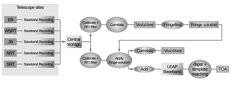
Figure 1: A flowchart of the LEAP data processing pipeline. Each observatory stores the baseband data from single-telescope LEAP observations on disk. The data are then transferred to the central storage machine at Jodrell Bank Observatory. There, polarization calibration and RFI mitigation filters are applied to the single-telescope data, which are then correlated, resulting into a fringe-solution for each of LEAP’s baselines (ten telescope pairs in total). At this stage, we apply the fringe-solution to each telescope’s baseband data (again after polarization calibration and RFI mitigation), correlate the time-series again, and check the resulting ‘visibilities’ to verify that the fringe-solution is indeed correct. The baseband data (to which the fringe-solution is applied) are then added together in phase, forming the LEAP tied-array. The added baseband data are processed as normal timing data. The data is then dedispersed and folded (using DSPSR) and template matching is performed to produce the final pulse times-of-arrival (TOAs).

4.1 Data processing pipeline

A flowchart of the LEAP processing pipeline is shown in Fig. 1. The processing starts once the baseband data of each 16 MHz subband from all LEAP telescopes from one of the observing sessions are online at the central storage machine at Jodrell Bank Observatory.

During the first processing stage, the data from each telescope are correlated to find the exact time and phase offsets between the telescopes. This is achieved by first applying an initial time offset corresponding to the geometric delay, the clock delay and the hardware delay by simply shifting one of the time-series by an integer number of samples with respect to the other. The remaining time delay is a fraction of a time sample (see § 4.2). The baseband data are then Fourier-transformed (channelized) to the frequency domain to form complex frequency channels. This is performed in time segments of typically 100 samples, leading to 100 frequency channels for each time-segment. The polyphase filters implemented in the digital instruments at Effelsberg, Jodrell Bank, Nançay and Sardinia provide complex valued time-series, requiring the complex-to-complex Fourier transform to channelize the data. In the case of WSRT, real-valued time-series are created and the real-to-complex Fourier transform is used to generate the channelized complex time-series. When converted to the frequency domain, the polarization is converted from linear to circular and the polarization calibration is applied (§ 4.3). At this stage the RFI mitigation methods are also applied (§ 4.5). The remaining fractional delay is corrected for by rotating the complex values of each frequency channel in phase. The corresponding complex time-series for each baseline pair and frequency channel are then correlated to form ’visibilities’. As such, the correlator is of the FX design, where the Fourier transform (F) is followed by the correlation (X), similar to other software correlators like DiFX (Deller et al., 2007) and SFXC Keimpema et al. (2015).

The visibilities are averaged in time, allowing the residual time and phase offsets between each pair of telescopes to be extracted by applying the global fringe fitting method from Schwab & Cotton (1983). An initial Fourier transform method is used to find a fringe solution to within one sample. This solution is then applied to a least-squares algorithm that makes use of phase closure and involves minimizing the difference between model phases and measured phases by solving for the phase offset of each telescope (fringe phase), the time slope (fringe delay) and the phase drift (fringe rate). The fits are performed independently on both left-hand-circular and right-hand-circular polarizations. The resulting fringe rates are averaged over both polarizations.

During the second processing stage, the exact time and phase offsets with respect to a reference telescope are applied to the baseband data from each telescope. An amplitude scaling is also applied to these data to ensure maximum sensitivity (see Sect. 4.4).

4.2 Phase calibration and pulsar gating

Creating the LEAP tied-array beam requires the baseband data from each telescope to be corrected for an appropriate time delay and phase shift before they can be added coherently. The time and phase delays between the time-series from individual telescopes consists of four components. First, the largest delays are due to differences in geometry that result in different path lengths that the signal has to travel. Second, there are differences between each observatory’s local clocks. The third component consists of instrument-specific delays due to cables and electronic components. Finally, the atmosphere (both ionosphere and troposphere) introduces a delay as a time-varying phase-shift of the radio-wavefront, which depends on the time-varying conditions of the local atmosphere as well as the wavelengths of the radio waves.

The geometric delays can be largely corrected for by using the known terrestrial positions of the telescopes, telescope pointing models and celestial position of the source (calibrator or pulsar). The long baselines in LEAP mean that our tied-array beam is very small and it is therefore essential to have an accurate position for the right epoch. It is therefore vital to include any known proper motion terms when calculating the true position for the observing epoch. For LEAP, these delays are calculated using the CALC program (Ryan & Vandenberg, 1980). For our pipeline, we make use of a C-based wrapper for CALC, which is part of the DiFX software correlator (Deller et al., 2007). Applying the geometric delays and clock delays requires a reference location and a reference time standard. We have chosen to reference the time series of the individual telescopes to the Effelsberg telescope. This choice was made primarily because the Effelsberg telescope is the one with the largest aperture. Because the time and phase delays are determined on baselines that include Effelsberg, the corrections are relative, not absolute. As a consequence, the corrected and subsequently added baseband time-series can be treated for further analysis as if they were observed by Effelsberg in terms of the geometric delays and clock offsets normally used in pulsar timing.

The delays from the signal-path and the atmosphere are measured by correlating the baseband data of the telescopes using the purpose-built LEAP software. An initial fringe-solution of the residual time and phase differences between each pair of telescopes is found by correlating a calibrator source. However, the calibrator source is typically offset by about 5^∘ from the pulsar and separated in time by several minutes. Because of this, the conditions of the ionosphere/troposphere for the calibrator observation will be different than for the pulsar observation, leading to a different fringe-solution. Thus, when the fringe-solution from the calibrator is applied to the pulsar data, it does not yield perfect coherence (see Fig. 2). In addition, the conditions of the ionosphere/troposphere can change unpredictably on a timescale of minutes, as shown in Fig. 3. This means that the observation would need to be interrupted to observe the calibrator at least once every 15 minutes (or even every 5 minutes in case the ionospheric conditions are very poor). As part of the processing pipeline, we therefore developed a procedure to allow the phase-calibration to be performed on the pulsar signal itself. This method of calibrating on the target is called self-calibration and widely used in interferometry.

To do this, we implemented a pulse binning technique to optimize the sensitivity. The visibilities within each individual pulse are integrated into bins with a size equal to a fraction of the pulse period. This is done for each frequency channel. The bins from each individual pulse are then added (folded) to the corresponding bins from all previous pulses, using TEMPO to predict the exact pulse period. A time-shift is applied to each individual channel to correct for the dispersion delay. This results in average visibilities for each pulsar phase bin, for each frequency channel and for each baseline. Finally, the bins containing the on-pulse signal are selected (this is the process of gating) and averaged together. This yields visibilities for each baseline where only the on-pulse signal of the pulsar contributes, and increases the signal-to-noise ratio roughly by a factor equal to the reciprocal of the square-root of the duty cycle. This procedure allows the fringes to be tracked over time on the pulsar signal itself as the conditions of the ionosphere/troposphere change, removing the need to switch between pulsar and calibrator during the observation. Phase calibrating on the target source uses the positional information of the pulsar, and hence this approach can not be used for astrometry.

Once the total time and phase delays for each telescope with respect to the reference telescope have been determined, they are applied to the raw data in two stages. First, the baseband data from each telescope are aligned to the nearest integer sample (62.5 ns for a complex sampled subband of 16 MHz). The remaining fractional time delay (a fraction of a sample) plus the measured delay in phase, is corrected for by phase rotating the complex values of the channelized time-series. After these corrections, the channelized time-series from each telescope correspond in both time and phase with the time-series from the reference telescope. These channelized time-series can thus be added together coherently.

Finding a fringe-solution after correlating the time-series from the telescopes can be impeded by a lack of pulsar signal, rapidly changing conditions of the ionosphere/troposhere, extreme cases of RFI, or – in the case of Nançay – by an irregular clock-drift. In those instances where no fringe-solution can be obtained, the time-series are added incoherently. The time series are then corrected for the known time-delays by applying the geometric delay correction, the clock correction, the instrumental delays and the fringe-solution from the calibrator, which aligns the signals to within a few tens of ns. Once the signals are time-aligned, they are added without consideration of the relative phase of the electromagnetic signal received by the individual telescopes. This is achieved by simply adding the power of the baseband data. For incoherent addition, the signal-to-noise ratio increases with the square-root of the number of added telescopes.

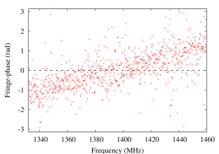
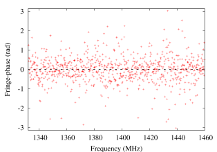
Figure 2: Fringe solution from a calibrator versus the fringe solution from the pulsar itself. These two panels show the visibility phase between the baseband time-series from Effelsberg and WSRT from the first 5 minutes of an observation of PSR J1022+1001, taken on February 24, 2015. The x-axis shows the observing frequency from 1332 to 1460 MHz. The y-axis shows the visibility phase between the two time-series for each frequency channel (in units of radians). The top graph shows the visibility phase from the calibrator (taken 6 min before the pulsar observation), applied to the pulsar observation. The bottom graph shows the fringe from the pulsar observation itself. A visibility phase of zero over the whole bandwidth means that the two signals are perfectly in phase and will thus add fully coherent. A residual time-offset between the two time-series will show up as a slope. The phase-calibrator is offset from the pulsar by $3^{\circ}$ on the sky.

Figure 3: The evolution of the fringe-phase over time. The four lines show the drift in the fringe-phase in radians of a calibrator observation for the two baselines Effelsberg-Jodrell Bank and Effelsberg-WSRT for both polarizations: left-hand circular (LHC) and right-hand circular (RHC). It demonstrates that both the absolute value of the fringe-phase as well as the time-derivative of the fringe-phase (called fringe-drift) can change significantly on a timescale of minutes.

4.3 Polarization calibration

To maximize the coherency of the tied-array beam, it is crucial to perform accurate polarization calibration that removes the effects introduced by the telescope, receiver and instrument. This is particularly important for LEAP, as each of the individual telescopes is of a different design, uses different receivers and feeds, and we are observing pulsars for which parts of the average pulse profiles are up to 100%-polarized. In Fig. 4 we compare uncalibrated pulse profiles with profiles after calibration using the method described below.

Here we briefly describe the LEAP polarization calibration scheme, the details of which will be presented in a forthcoming paper. In LEAP, polarization calibration is performed for each telescope independently, before correlating and finding the fringes. Performing polarization calibration has two major benefits. First, it helps to improve the S/N of fringe solutions, i.e. to determine accurate phase offsets between telescopes. Second, performing polarization calibration after coherent addition is complicated, since extra phases have been introduced in the addition process. In fact, the expected S/N of an un-calibrated fringe will be 22% lower than the calibrated one, assuming random differential phase between the two hands of polarization and a 100% polarized signal. It is thus hard to evaluate the polarization performance of each telescope, and check the data integrity individually.

For single telescope systems, the distortion of polarization can be described by seven system parameters. For a quasi-monochromatic wave, there are two major parametrization schemes. In Britton’s scheme (Britton, 2000), there are: the total gain, spinor transformation axes (four parameters) and the transformation rotation angles (two parameters). In Hamaker’s scheme (Hamaker et al., 1996), there are: the total gain, the gain-phase imbalance (two parameters), leakage amplitude and phase (four parameters). The two descriptions are equivalent. We adopt the Hamaker scheme in the LEAP pipeline, however we do not assume that the polarization distortions are small, since we are working with an inhomogeneous array.

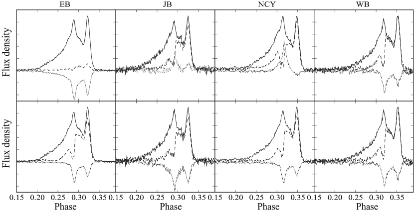
Figure 4: Pulsar profiles of PSR J1022+1001 as observed with the individual telescopes before and after polarization calibration. The solid, dashed, and dotted curves, are for total intensity, linear polarization, and circular polarization respectively. The top row are the profile without calibration, and the bottom row are the calibrated ones. The EB, JB, NCY, and WB abbreviations indicate the Effelsberg, Jodrell, Nançay, and Westerbork telescopes. Here the y-axis, flux, takes an arbitrary unit, and x-axis is pulse phase. The calibrated profiles clearly show much better consistency.

The aforementioned system parameters can be measured by comparing the observed full-Stokes pulsar pulse profile to the standard profile templates. The standard $\chi^{2}$ fitting minimizing the differences between the template and the modeled profile is used to fit for the system parameters of each frequency channel. In this way, the pulsar itself is also used as the polarization calibrator in our observations. PSR J1022+1001 and/or PSR B1933+16, for which the pulse profiles show significant amounts of both linear and circular polarization components, are normally used for polarization calibration. Our approach is similar to the matrix template matching method by van Straten (2006), except that we calibrate baseband data directly.

There are three major steps in our algorithm. First, the observed pulse profile is aligned with a template profile (using the algorithm of Taylor 1992). Next, non-linear $\chi^{2}$-fitting is used to derive the system parameters. These system parameters are then applied to the observed profile in order to estimate the post-calibrated profile. These steps are repeated until the solution converges, that is when the fractional changes of the system parameters are smaller than $10^{-7}$. Our results show that the above iteration converges most of the time, and that we can measure both the system parameters and the phase offsets between the template and measured pulse profile at the same time. This procedure is similar to using a noise diode as a calibrator. However, because of the change of polarization angle across the pulse profile, we are no longer limited to the case of single-axial calibration, and are able to fix the whole set of system parameters, including leakage terms. Indeed, we need to include such terms to fully calibrate the Nançay data. Figure 5 shows the improvement in visibility phases after calibrating the polarization.

Figure 5: This figure illustrates the effects of the polarization calibration for a 10-second integration of a 16 MHz subband of the Effelsberg-Nançay baseline. The top panel shows the visibility phase $\Delta\Phi$ as a function of frequency with and without applying of the polarization calibration. A histogram of these phase delays with and without applying the polarization calibration is shown in the bottom panel. For this example, the average S/N of the visibilities shows an 18% increase after polarization calibration, and the corresponding phase error is reduced by 40%, i.e. the rms level of the visibility phase reduced is from $35^{\circ}$ to $20^{\circ}$.

4.4 Amplitude calibration

To ensure maximum S/N of the added data, we have to apply an appropriate weight to the baseband data from each of the telescopes, where we have to consider that the final added data are written as 8-bit samples. To achieve this, we select a reference telescope and measure the noise-levels from the baseband data from each telescope and set the weights such that all samples are scaled to the noise-levels of the reference telescope. We then take the S/N from the average intensity profiles from the individual telescopes and scale the weights with an additional factor given by:

$$W_{\mathrm{tel}}=\sqrt{\frac{\mathrm{S/N}_{\mathrm{tel}}}{\mathrm{S/N}_{\mathrm{ref}}}},$$

where $\mathrm{S/N}_{\mathrm{tel}}$ is the S/N of the telescope and $\mathrm{S/N}_{\mathrm{ref}}$ is the S/N of the reference telescope. This ratio of the S/N includes the telescopes’ system temperature relative to that of the reference telescope. The voltage samples from each of the telescopes are then multiplied by the corresponding weight before the addition, which maximizes the S/N of the added data. At this stage, the samples are floating point numbers. After the addition, a final scaling is applied such that the standard deviation of the samples becomes one third of the dynamic range of 8-bit data. This ensures minimal clipping and optimal use of the dynamic range when the data is converted to 8-bit and written to disk.

4.5 Interference mitigation

In case of significant radio frequency interference (RFI), we have implemented two methods to clean the data. The RFI mitigation step is optional and performed right after the calibration. These RFI mitigation methods are applied to the channelized data from the individual telescopes before coherent addition.

The first form of RFI-mitigation consists of selecting and masking frequency channels that contain narrow-band RFI. These channels are selected via a simple algorithm that looks for channels with an integrated power exceeding either a given threshold or deviating significantly from its neighbors. These channels are then masked by replacing the content with Gaussian noise with mean and rms determined from neighboring time samples.

A second technique can be applied to data containing time-varying RFI, or broadband RFI. This technique implements the method of spectral kurtosis (Nita & Gary, 2010a, b) to remove RFI from some observations. It provides unbiased RFI removal with a resolution of 6.25 ms in time and 0.16 MHz in frequency. In each frequency channel and at each telescope, the distribution of a time-series of 1000 samples of total power is assessed for similarity to that expected from Gaussian-distributed amplitudes. This is done using an estimator that measures the variance divided by the square of the mean for these power samples. When the power is derived from Gaussian amplitudes of zero mean, the estimator has a probability density function (PDF) that is independent of the variance of those amplitudes. It can therefore be used to distinguish RFI on the premise that non-Gaussian amplitudes are caused by RFI. The PDF is used to determine three-sigma limits for the estimator, and a block of 2000 amplitude samples (1000 in each polarization channel) is masked if it gives an estimator value outside these limits. This excludes $0.27\%$ of RFI-free data, while excluding most RFI-contaminated data. The amplitudes of RFI-contaminated samples are replaced by artificial Gaussian noise with the same variance as nearby samples, in order to maintain a constant noise level in the correlated amplitudes regardless of the number of telescopes contributing to each sample. As before, the masked data is replaced by Gaussian noise.

We cannot generally define the percentage of RFI-contaminated data that is excluded, because we do not know, a priori, the PDF of the estimator derived from these data. Some RFI-contaminated data may not be excluded if their PDF closely mimics that of Gaussian amplitudes. However, our practical application has shown it to be effective in automatically removing the vast majority of the dominant RFI that would otherwise spoil our correlations (see Fig. 6). It is also possible that a very strong pulsar signal could be misinterpreted as RFI by the spectral kurtosis method but that does not happen when using the time and frequency resolutions employed by LEAP.

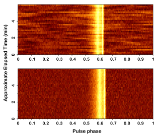
Figure 6: Pulsar phase-vs-time plot of coherently-added LEAP data of PSR J1022+1001, without (top) and with the spectral kurtosis RFI mitigation method (bottom). The observation was taken on July 27, 2013 with Effelsberg, Jodrell Bank, Nançay, and WSRT. There was significant broadband RFI from the Nançay observation, which dramatically changed the baseline of the coherently-added integration profile, as shown in the top panel. After applying the filter to Nançay data only, the resulting LEAP data are significantly improved.

Table 1: Pulsars and calibrators observed for the LEAP project. Notes: a) PSR J1518$+$4904 cannot be observed simultaneously with all five telescopes, therefore the Jodrell Bank, Effelsberg, and Sardinia telescopes observe PSR J1738$+$0333 instead. b) PSR B1933$+$16 is used for polarization calibration as explained in Sect. 4.3 and is not included in the PTA list. Telescope codes: E: Effelsberg; J: Jodrell Bank; N: Nançay; S: Sardinia; W: WSRT.

Pulsar	Calibrator	length (min)	telescopes	Pulsar	Calibrator	length (min)	telescopes
	J0029+0554	3	EJNSW		J1719+0817	3	EJNSW
J0030+0451		40	EJNSW	J1713+0747		50	EJNSW
	J0037+0808	3	EJNSW		J1719+0817	3	EJNSW
	J0606$-$0024	3	EJNSW		J1740+0311	3	EJS
J0613$-$0200		60	EJNSW	J1738+0333a		60	EJS
	J0616$-$0306	3	EJNSW		J1740+0311	3	EJS
	J0619+0736	3	EJSW		J1740$-$0811	3	EJNSW
J0621+1002		45	EJSW	J1744$-$1134		45	EJNSW
	J0619+0736	3	EJSW		J1752$-$1011	3	EJNSW
	J0743+1714	3	EJSW		J1821$-$0502	3	EJNSW
J0751+1807		40	EJSW	J1832$-$0836		35	EJNSW
	J0743+1714	3	EJSW		J1832$-$1035	3	EJNSW
	J0927$-$2034	3	EJNSW		J1847+0810	3	EJNSW
J0931$-$1902		40	EJNSW	B1855+09		50	EJNSW
	J0932$-$2016	3	EJNSW		J1847+0810	3	EJNSW
	J0957+5522	3	EJSW		J1926$-$1005	3	EJSW
J1012+5307		45	EJSW	J1918$-$0642		20	EJSW
	J0957+5522	3	EJSW		J1926$-$1005	3	EJSW
	J1015+1227	3	EJNSW		B1933+16b	5	EJNSW
J1022+1001		45	EJNSW	B1937+21		45	EJNSW
	J1025+1253	3	EJNSW		J1946+2300	3	EJNSW
	J1028$-$0844	3	EJSW		J2006$-$1222	3	EJNSW
J1024$-$0719		45	EJSW	J2010$-$1323		55	EJNSW
	J1028$-$0844	3	EJSW		J2011$-$1546	3	EJNSW
	J1506+4933	3	NW		J2130$-$0927	3	EJNSW
J1518+4904a		60	NW	J2145$-$0750		45	EJNSW
	J1535+4957	3	NW		J2155$-$1139	3	EJNSW
	J1554$-$2704	3	EJNSW		J2232+1143	3	EJNSW
J1600$-$3053		60	EJNSW	J2234+0944		35	EJNSW
	J1607$-$3331	3	JNSW		J2241+0953	3	EJNSW
	J1641+2257	3	EJSW		J2303+1431	3	EJNSW
J1640+2224		50	EJSW	J2317+1439		40	EJNSW
	J1641+2257	3	EJSW		J2327+1524	3	EJNSW
	J1638$-$1415	3	EJNSW
J1643$-$1224		35	EJNSW
	J1638$-$1415	3	EJNSW

5 Observing strategy

LEAP observations are crucial in that they complement the regular, more frequent multi-frequency observations of the EPTA by adding time-of-arrival measurements with the highest possible precision. Observing sessions for LEAP are scheduled with an approximately monthly cadence, each session lasting a minimum of 24 hours. During each observing session, a set of millisecond pulsars and phase calibrators are observed simultaneously with each of the five radio telescopes. Since the first observations of June 2010, the observing time per session, number of pulsars per session, and number of participating telescopes per session have steadily increased.

Initial testing to aid in software development used eight of the single 25-m WSRT dishes, obtaining 20 MHz of bandwidth for a set of 6 millisecond pulsars. These data were used to test software beamforming and allow a comparison with the output of the WSRT hardware beamformer. The first long-baseline observations were obtained in June 2011 using WSRT and Effelsberg. These observations initially used five subbands of 20 MHz, but switched to the $8\times 16$ MHz setup starting in February 2012, when the Lovell telescope at Jodrell Bank was included in the LEAP array. The Nançay telescope first joined in May 2012, initially with $4\times 16$ MHz subbands, and since December 2012 with the full 128 MHz bandwidth. Test observations with the SRT were obtained in July 2013 for one 16 MHz subband. Tests with one subband were then performed monthly until January 2014. Finally, thanks to the successful installation of an 8-node computer cluster, the telescope joined full-length and full-bandwidth LEAP sessions in March 2014.

Through a memorandum of understanding between the participating telescopes and institutes, observing time at Jodrell Bank, Nançay and SRT is guaranteed, while for Effelsberg and WSRT, the observing runs are proposed through the peer-review process at these telescopes. The long-term scheduling at Effelsberg and WSRT thus guides the scheduling of the LEAP observing sessions, which are matched by the Lovell, Nançay and Sardinia telescopes.

Besides the principal requirement that the observed sources be simultaneously visible from all sites, the observing schedule takes the individual telescope constraints into account for each LEAP session. The primary observing constraint is set by the transit design of Nançay, where sources are visible for 60 to 90 minutes around culmination, depending on the declination of the source. The altitude-azimuth mounts of the Effelsberg, Lovell and Sardinia telescopes usually do not allow observations at very small local zenith-angles (i.e. LEAP observations avoid zenith angles of less than 10^∘), and have slew limits at certain azimuths related to cable wrapping. The equatorial design of WSRT limits observations to hour angles from $-6$ to $+6$ h around transit for each source. Furthermore, WSRT requires a 3-min initialization time between observations to configure the tied-array. This initialization time overlaps with the slewing time for all telescopes, as well as with a minimum observing length requirement of 6 min for all observations done with the Lovell Telescope. The slewing rates, minimum observing time and initialization time mostly impact the calibrator observations before and after each pulsar observation, which are generally only three minutes long. To obtain the most efficient overall observing schedule and a maximum overlap between all telescopes for each observation, LEAP requires all observations to end at the same time.

Besides the telescope constraints, the visibility of MSPs suitable for pulsar timing array experiments also provides a stringent constraint on the schedule. To first order, the most suitable pulsars are clustered towards the inner Galactic plane, with very few pulsars at right ascensions between $01^{\mathrm{h}}$ and $05^{\mathrm{h}}$. Furthermore, to maximize the number of sources that are visible at Nançay, it is beneficial to include sources separated equally in right ascension. To maximize the number of suitable MSPs observable by LEAP, we moved away from continuous 24-hour observing sessions. Since the spring of 2013, we observe in two sessions, spanning right ascension ranges from $06^{\mathrm{h}}00^{\mathrm{m}}$ to $01^{\mathrm{h}}30^{\mathrm{m}}$ and $15^{\mathrm{h}}30^{\mathrm{m}}$ to $21^{\mathrm{h}}00^{\mathrm{m}}$. The two parts of a full LEAP run are usually separated by only a day. Table 1 lists the pulsars and phase calibrators observed by LEAP. The current selection of pulsars is based on an optimization of using the best pulsars observed by the EPTA (Desvignes et al. submitted), while following the observing restrictions explained above. This results in some high-quality pulsars in crowded areas of the sky being observed by less than 5 telescopes, or not being included at all; this also means that some pulsars that are not necessarily the best PTA sources are included in the list.

6 Results

Processing of LEAP data is presently ongoing. During the second half of 2014 the processing pipeline reached a level of maturity that allowed us to transition to a scheme whereby the data of one epoch was processed and analyzed before the data of the next epoch was obtained. Here, we present results obtained from data from these epochs, as well as data from a few specific epochs prior to the second half of 2014, which have been processed during the development phase of the pipeline.

6.1 Coherence

The correlation and addition of single-telescope baseband data using the LEAP data reduction pipeline produces LEAP data with the expected coherence. An example of such coherence is shown in Fig. 7, where we present the pulse profile of PSR J1022+1001 from LEAP data compared to the profiles from single-telescope data (all scaled to the off-pulse rms). In Fig. 8 we present the S/Ns of all the LEAP profiles for PSR J1022+1001, compared to those of the individual dishes, for the months in which the pulsar signal was strong enough to perform coherent addition. Full coherent addition is achieved when the time series of the individual telescopes are perfectly in phase. The LEAP S/N should then be similar to the sum of the S/Ns of the individual telescopes. Fig. 7 and 8 show that the S/N for LEAP is close to the sum of the S/Ns of the individual telescopes, demonstrating that LEAP is achieving full coherent addition when there is sufficient signal. Deviations from the maximum S/N can be caused by an inaccurate fringe-solution (possibly due to residual RFI or due to a non-linear phase-drift), or due to improper polarization or amplitude calibration (see Sect. 4.3 and 4.4).

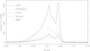
Figure 7: Pulsar profiles of PSR J1022+1001 from individual telescopes and their coherent addition, normalized based on their off-pulse rms. The raw data were obtained at MJD 56500, with an integration time of 30 minutes. The peak signal-to-noise ratios of Effelsberg, Jodrell Bank, Nançay, WSRT and LEAP, are 97, 51, 42, 30, 220, respectively, which corresponds to a near perfect coherency.

With LEAP observing there are three possible data combinations. The most sensitive of these is clearly when we combine all the dishes involved coherently over the full LEAP bandwidth. In the few cases where coherent addition is not possible the incoherent sum of the available dishes, over the LEAP bandwidth, gives us the best sensitivity. This assumes that a sufficient number of dishes (i.e. more than 2) is involved in the sum. Otherwise, the incoherent combination of the TOAs, as opposed to the raw data, from the wide bandwidth observations from the individual telescopes is used. This is because the sensitivity of the incoherent sum scales as the square-root of the number of dishes while the sensitivity of the combination of the TOAs determined from the wide-band data scales as the square-root of the ratio of the bandwidth available to the dishes over that available to LEAP. In all cases we end up with a better result for the overall sensitivity compared to what would be possible with a single telescope observation from one of the LEAP dishes.

Based on the LEAP observations that have been fully processed at the time of submission of this paper, 51% of the sources were processed coherently with more than 80% coherency, 8% were processed coherently with 60 to 80% coherency, and the remaining 41% were processed incoherently. The reasons for the poor coherency achieved for some of the pulsars are a combination of poor S/N due to scintillation, imperfect polarization calibration, large or non-linear fringe drifts due to ionospheric conditions or the Nançay clock, and RFI across the LEAP band.

While these coherence numbers are lower than hoped, we have already improved our polarization calibration routines and our RFI mitigation procedures as described elsewhere in the paper, therefore these statistics are already improving. As discussed above, even if full coherence is not achieved, the various forms of incoherent combination already result in significant improved TOA precision compared to an observation with a single EPTA telescope. However we also do see ways to improve our ability to achieve coherence more often and discuss some of them here. When using the pulsar for fringe-finding we use pulsar gating, that is we use only the on-pulse region to improve the S/N, to further improve this we will subtract the off-pulse region which can improve sensitivity in regions of the sky where there might be bright sources in the field-of-view of one or more of the telescopes. We will also implement a new algorithm for identifying the on-pulse region when the pulsar has low S/N which will use the predicted phase of the pulse and a template profile. The long baselines mean that ionospheric conditions can lead to significant phase drift as a function of frequency, as can the less stable clock at Nançay. One way to overcome this is to implement a more sophisticated fringe-fitting routine which searches over a range of fringe-drift rates to look for the best drift rate to maximise the S/N of the fringe detection without having to go to too short integration times. Another option we are investigating for the near future is to increase the bandwidth used for LEAP. Not only does this lead to a higher S/N through the increased bandwidth, it also increases the chance of detecting the pulsar when it scintillates over a bandwidth smaller than the observed bandwidth. This improves our chances of getting coherent solution in that part of the band, but the delays can also be used to search for fringes where the signal is weaker. So overall the prospects are good for significantly improving the coherence that can be achieved for LEAP.

Figure 8: S/Ns from LEAP vs. S/Ns from the individual telescopes for PSR J1022+1001 for the observations where coherent addition could be performed. The earliest observation shown is from February 2012, the last observation shown is from February 2015. The graph shows that the LEAP data provides the expected improvement in S/N, meaning that the sum of the S/Ns of the individual telescopes is roughly identical to the S/N of LEAP.

6.2 Improvement in timing accuracy

The LEAP coherent addition makes optimal use of the acquired radio signals from each individual telescope. At present it uses a smaller bandwidth than in ordinary EPTA timing observations at most telescopes. This is in part due to the limited bandwidth available with PuMa II at the WSRT, but also due to current limitations on data rates and data storage. In the future we plan to expand the bandwidth observed with LEAP. To demonstrate that LEAP can improve the data quality, as compared to the individual telescope observations with wider bandwidth, we compare the LEAP TOAs of PSR J1022+1001 with those from single telescopes (see Fig. 9). The TOAs from Jodrell Bank and Nançay were derived directly from the simultaneous observations in ordinary timing mode, with bandwidths of 400 and 512 MHz, respectively, while SRT TOAs are limited to the LEAP bandwidth (128 MHz). The TOA uncertainties from Effelsberg and WSRT were extrapolated based on the LEAP bandwidth to 200 MHz and 160 MHz, respectively, since data acquisition with a wider bandwidth is not feasible at these telescopes during LEAP observations. It can be seen that compared with regular timing observations at the individual telescopes, the TOAs obtained from coherently-added LEAP data have smaller uncertainties. This is even more striking when one considers that the observations at Jodrell Bank and Nançay observe over the same full 400 and 512 MHz bandwidth as regular timing observations. The bands that are not used for coherent addition are dedispersed and folded as if they were regular timing observations, hence contributing to the timing dataset of those particular telescopes. Therefore, observations in LEAP mode clearly improve the sensitivity compared to the individual telescopes, as expected.

Furthermore, in Fig. 10 we compare the TOAs of PSR J1713+0747 determined from both the individual telescope data as described above, as well as the LEAP coherent sum, with the long-term EPTA timing solution (Desvignes et al. submitted). This timing solution is based on data from the individual telescope participating in the LEAP project (Effelsberg, Jodrell Bank, Nançay and WSRT) and obtained over a 17.7 year long timespan between October 1996 and June 2014. The data for the long-term EPTA timing solution were obtained with older generation instruments. No parameters in the timing solution were fitted for except for timing offsets between the individual telescopes. Fitting only for these timing offsets yields a solution with an rms of 0.25 $\mu$s when using TOAs from both the individual and coherently added LEAP data spanning nearly 4 years. Using only TOAs from the coherently added LEAP data improves the rms to 0.18 $\mu$s. For comparison, the long-term EPTA timing solution has an rms residual of 0.68 $\mu$s over the 17.7 year observing span (Desvignes et al. submitted). The TOAs determined from individual telescope data significantly improve the timing precision, primarily due to the use of a new generation of instruments, capable of coherent dedispersion over larger bandwidths. The TOAs determined from coherently combined LEAP data provide a further improvement on top of that.

Figure 9: TOA uncertainties from LEAP for PSR J1022+1001 compared with those obtained from single-telescope data, which were acquired simultaneously but with broader bandwidth. The full ordinary bandwidths of Jodrell Bank and Nançay are 400 and 512 MHz, respectively. The TOA uncertainties from Effelsberg and WSRT were extrapolated from 128 MHz to 200 and 160 MHz, respectively (these are the bandwidths used in the ordinary on-site EPTA timing campaigns). The available EPTA timing bandwidth at SRT is currently the same as LEAP.

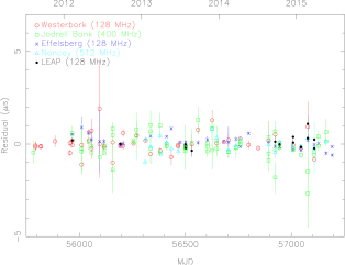
Figure 10: Timing residuals of PSR J1713+0747 obtained from single telescope data (colored points), as well as the coherently added LEAP data (black points). These residuals are computed by comparing the TOAs against the long-term EPTA timing solution of PSR J1713+0747 (Desvignes et al. submitted). No parameters, other than timing offsets between the telescopes, were fitted for. Over this five year timespan the data from the individual telescopes participating in LEAP, as well as the coherently added LEAP data presently available, allow the timing solution to be constrained to an rms of 0.25 $\mu$s. The solution using only TOAs determined from the coherently added LEAP data has an rms of 0.18 $\mu$s. For the Jodrell Bank and Nançay telescopes the TOAs from the data obtained over the full instrument bandwidth are shown.

6.3 Phase jitter and single pulse studies

LEAP delivers a sensitivity that is rivaled only by Arecibo, the largest single-dish radio telescope on Earth. The data are therefore ideal for studies of the phase jitter of integrated profiles and single pulses of MSPs, which are not often feasible with single-telescope data due to low S/N. Fig. 11 shows an example of such an analysis for PSR J1713+0747. The observations were carried out with Effelsberg, Nançay, and WSRT on MJD 56193. The plot shows timing residuals for 10-s integrations for a 15-min observing time. The TOA errors corresponding to measurement uncertainties due to radiometer noise were estimated by the classic template matching method (Taylor, 1992). To calculate the residuals, we used the ephemeris from the EPTA timing release (Desvignes et al. submitted) without fitting for any parameters. We see that the error bars clearly underestimated the scatter of the residuals, which is an indicator of phase jitter (e.g. Liu et al., 2011). The rms residual is 522 ns with a reduced $\chi^{2}$ of 9.47. Following the method in Liu et al. (2012), this leads to an estimated jitter noise of 494 ns for a 10-s integration time. This is consistent with previously published results (Shannon & Cordes, 2012; Dolch et al., 2014). From the coherently-added LEAP data, we also managed to obtain single pulses of the pulsar with fully-calibrated polarization at a time resolution of 2.2 $\mu$s, an example of which can be found in Fig. 12. The single pulses have sharp features and significant linear polarizations. Further investigation of the single pulses from PSR J1713+0747 will be presented in a separate paper.

Figure 11: Timing residuals of PSR J1713+0747 over a period of 15 min, for each 10-s integration. The observations were performed on MJD 56193, included Effelsberg, Nançay, and WSRT, and the generation of the LEAP data achieved a coherency of 95%. The rms residual is 522 ns and the corresponding reduced $\chi^{2}$ is 9.47.

Figure 12: Polarization profile of a single pulse from PSR J1713+0747, obtained from the observation used in Fig. 11.

6.4 Pulsar searching

The increased sensitivity of the LEAP tied array allows searches for weak pulsars with known positions. Though the LEAP tied array beam of the full LEAP array is small, beamforming can be used to tile out the incoherent beam.

As a proof of concept, we have performed a blind search on 5 min of coherently-added LEAP data of the double neutron star PSR J1518+4904, with the aim of detecting pulsations from the second neutron star. The baseband data were acquired at MJD 56193 with Effelsberg and the WSRT, and were later combined with nearly full coherency. The resulting Nyquist-sampled timeseries of each 16-MHz subband were then used to form a filterbank file with 1-MHz channels. Next we combined the filterbank files from each individual subband to yield the full observing bandwidth and used the PRESTO software package to search for pulsations.

In total, 33 candidates were detected with the same DM as PSR J1518+4904, all of which were harmonics of the pulsar or attributed to RFI. No pulsations with a non-harmonic period were found from an initial investigation down to a flux limit of 0.31 mJy. As PSR J1518+4904 is part of the monthly LEAP observing sessions, we will be able to use all coherently-combined data on this system for the most sensitive search to date for radio emission from its neutron star companion.

7 Conclusions and prospects

In this paper we present an overview of the LEAP project, which coherently combines data from up to five 100-m class radio telescopes in Europe, forming a tied-array telescope. We observe a subset of the EPTA MSPs with a sensitivity that cannot be achieved by the individual participating telescopes. The LEAP project emerges as a natural result of the many years of collaboration between the EPTA groups. Instead of merely sharing their TOAs for GW detection purposes, the EPTA telescopes in the LEAP project are combined using VLBI techniques to form a fully-steerable 195-m equivalent dish, forming one of the most sensitive pulsar observation instruments to date.

We describe the LEAP setup and operation, starting from the data acquisition setup at the participating telescopes, the transfer of data to the centralized LEAP computing infrastructure at Jodrell Bank, to the final processing of the monthly LEAP observing runs. We have also presented the main characteristics of the pipeline that was developed for the processing the data. We describe the challenges of achieving high timing precision, in great part due to the many differences in the telescopes and their pulsar observing systems. These differences were managed either fully in software (incorporated into the LEAP pipeline), or with hardware upgrades when these were inevitable. The development of our own end-to-end pipeline (individual telescope data, polarization calibration, RFI mitigation, correlator and tied-array adder) not only provided us with the flexibility to overcome all of these obstacles, but also allowed us to take the most out of each telescope. The efforts placed into making LEAP a reality have however been rewarded by the quality of the results. As we have shown, the coherency of the added individual telescope data can reach 100%. In addition, the TOA uncertainty of the LEAP data is less than that of the individual telescopes, even though the LEAP bandwidth is a few times smaller.

Although the main aim of LEAP is to provide high precision pulsar timing data towards a direct detection of GWs, its high sensitivity and flexibility as an observing system enable it to go beyond this scope and pursue broader pulsar-related science. Pulse phase jitter and single pulse studies, which are demanding in terms of sensitivity, are ideal for LEAP. This was best demonstrated with the single pulse detections of PSR J1713+0747 during one of the standard LEAP observations. We have also demonstrated that LEAP is capable of performing targeted pulsar searches in a case study using PSR J1518+4904. Even though its current operation mode does not allow it to be used as a generic pulsar searching instrument, its high sensitivity makes it a perfect tool for investigating known binaries and looking for pulsations from pulsar companions in order to identify double-pulsar systems. Moreover, LEAP has recently been used to observe the Galactic center magnetar PSR J1745$-$2900 at frequencies higher than used in the typical LEAP runs, in order to determine the scattering properties of the ISM towards the Galactic centre. This study used VLBI imaging techniques and helped define the best search strategies for pulsars close to Sgr A^∗ (Wucknitz, 2015).

The addition of LEAP data to the current PTA data sets will significantly improve PTA data quality. We are currently finalizing the LEAP timing data set of the data obtained to date, and will use these data to perform a search for GWs and place upper limits on the GW amplitude. We can already extrapolate the results of our currently processed data to the full time span of 3.2 years, by counting the number of telescopes that joined each observing session. Assuming 90% coherency and using the red noise parameters of each pulsar measured from the much longer EPTA data set, we can calculate the statistics of the expected timing noise and measurement accuracy, then derive upper limits on the amplitude of the GW background using a Cramer-Rao bound. For a spectral index of $-2/3$ (i.e. a stochastic GW background dominated by supermassive binary black holes), the LEAP upper limit on the dimensionless strain amplitude $A_{\mathrm{c}}$ is $A_{\rm c}({\rm 1yr^{-1}})\leq 1.2\times 10^{-14}$, using extrapolated data of four LEAP pulsars, PSR J0613$-$0200, J1022$+$1001, J1600$-$3053, and J1713$+$0747. With only 3.2 years of data, such an upper limit is a factor 2 to 5 higher compared to the published results that used 10-year long data sets and more pulsars (van Haasteren et al., 2011; Demorest et al., 2013; Shannon et al., 2013; Lentati et al., 2015).

Dedicated funding for the LEAP project officially ended in September 2014. However, the unique character and the success of LEAP have justified its continuation at all participating telescopes, which have provided the necessary monthly observation time. While this paper provides an overview of the LEAP project, several papers are presently in preparation that provide details of the instrumentation, pipeline and the calibration, as well as present results from the LEAP project.

References

- Aad et al. (2012) Aad G., Abajyan T., Abbott B., Abdallah J., Khalek S. A., 2012, Physics Letters B, 716, 1
- Abbott et al. (2009) Abbott B. P., et al., 2009, Reports on Progress in Physics, 72, 076901
- Accadia et al. (2012) Accadia T., et al., 2012, Journal of Instrumentation, 7, 3012
- Amaro-Seoane et al. (2013) Amaro-Seoane P., et al., 2013, GW Notes, Vol. 6, p. 4-110, 6, 4
- Baars & Hooghoudt (1974) Baars J. W. M., Hooghoudt B. G., 1974, A&A, 31, 323
- Britton (2000) Britton M. C., 2000, ApJ, 532, 1240
- Chatrchyan et al. (2012) Chatrchyan S., Khachatryan V., Sirunyan A., Tumasyan A., Adam W., Aguilo E., 2012, Physics Letters B, 716, 30
- Cognard et al. (2013) Cognard I., Theureau G., Guillemot L., Liu K., Lassus A., Desvignes G., 2013, in Cambresy L., Martins F., Nuss E., Palacios A., eds, SF2A-2013: Proceedings of the Annual meeting of the French Society of Astronomy and Astrophysics. pp 327–330
- Cordes & Shannon (2010) Cordes J. M., Shannon R. M., 2010, preprint, (arXiv:1010.3785)
- Deller et al. (2007) Deller A. T., Tingay S. J., Bailes M., West C., 2007, PASP, 119, 318
- Demorest et al. (2013) Demorest P. B., et al., 2013, ApJ, 762, 94
- Detweiler (1979) Detweiler S., 1979, ApJ, 234, 1100
- Dolch et al. (2014) Dolch T., et al., 2014, ApJ, 794, 21
- Grote & LIGO Scientific Collaboration (2010) Grote H., LIGO Scientific Collaboration 2010, Classical and Quantum Gravity, 27, 084003
- Hamaker et al. (1996) Hamaker J. P., Bregman J. D., Sault R. J., 1996, A&AS, 117, 137
- Hellings & Downs (1983) Hellings R. W., Downs G. S., 1983, ApJ, 265, L39
- Hobbs et al. (2010) Hobbs G., et al., 2010, Classical and Quantum Gravity, 27, 084013
- Janssen et al. (2014) Janssen G. H., et al., 2014, in Advancing Astrophysics with the Square Kilometre Array.
- Karuppusamy et al. (2008) Karuppusamy R., Stappers B., van Straten W., 2008, PASP, 120, 191
- Keimpema et al. (2015) Keimpema A., et al., 2015, Experimental Astronomy, 39, 259
- Kettenis & Keimpema (2014) Kettenis M., Keimpema A., 2014, in Proceedings of the 12th European VLBI Network Symposium and Users Meeting (EVN 2014). 7-10 October 2014. Cagliari, Italy.. p. 88
- Kramer & Champion (2013) Kramer M., Champion D. J., 2013, Classical and Quantum Gravity, 30, 224009
- Kramer et al. (2006) Kramer M., et al., 2006, Science, 314, 97
- Lentati et al. (2015) Lentati L., et al., 2015, MNRAS, 453, 2576
- Liu et al. (2011) Liu K., Verbiest J. P. W., Kramer M., Stappers B. W., van Straten W., Cordes J. M., 2011, MNRAS, 417, 2916
- Liu et al. (2012) Liu K., Keane E. F., Lee K. J., Kramer M., Cordes J. M., Purver M. B., 2012, MNRAS, 420, 361
- Manchester & IPTA (2013) Manchester R. N., IPTA 2013, Classical and Quantum Gravity, 30, 224010
- Manchester et al. (2013) Manchester R. N., et al., 2013, Publ. Astron. Soc. Australia, 30, 17
- Nita & Gary (2010a) Nita G. M., Gary D. E., 2010a, PASP, 122, 595
- Nita & Gary (2010b) Nita G. M., Gary D. E., 2010b, MNRAS, 406, L60
- Roy et al. (2012) Roy J., Bhattacharyya B., Gupta Y., 2012, MNRAS, 427, L90
- Ryan & Vandenberg (1980) Ryan J. W., Vandenberg N. R., 1980, in Bulletin of the American Astronomical Society. p. 457
- Schwab & Cotton (1983) Schwab F. R., Cotton W. D., 1983, AJ, 88, 688
- Shannon & Cordes (2012) Shannon R. M., Cordes J. M., 2012, ApJ, 761, 64
- Shannon et al. (2013) Shannon R. M., et al., 2013, Science, 342, 334
- Stappers et al. (2011) Stappers B. W., et al., 2011, A&A, 530, A80
- Taylor (1992) Taylor J. H., 1992, Royal Society of London Philosophical Transactions Series A, 341, 117
- Taylor & Weisberg (1982) Taylor J. H., Weisberg J. M., 1982, ApJ, 253, 908
- Thompson et al. (1991) Thompson A. R., Moran J. M., Swenson G. W., 1991, Interferometry and synthesis in radio astronomy
- Verheijen et al. (2008) Verheijen M. A. W., Oosterloo T. A., van Cappellen W. A., Bakker L., Ivashina M. V., van der Hulst J. M., 2008, in Minchin R., Momjian E., eds, American Institute of Physics Conference Series Vol. 1035, The Evolution of Galaxies Through the Neutral Hydrogen Window. pp 265–271 (arXiv:0806.0234), doi:10.1063/1.2973599
- Wucknitz (2015) Wucknitz O., 2015, ArXiv:1501.0451,
- van Haasteren et al. (2011) van Haasteren R., et al., 2011, MNRAS, 414, 3117
- van Straten (2006) van Straten W., 2006, ApJ, 642, 1004
- van Straten & Bailes (2011) van Straten W., Bailes M., 2011, Publ. Astron. Soc. Australia, 28, 1