Phonon contributions to ab initio double mass differences of magic nuclei

Abstract

Odd-even double mass differences (DMD) of magic nuclei are found within the approach starting from the free $NN$ interaction with account for particle-phonon coupling (PC) effects. We consider three PC effects: the phonon induced effective interaction, the renormalization of the “ends” due to the $Z$-factor corresponding to the pole PC contribution to the nucleon mass operator and the change of the single-particle energies. The perturbation theory in $g^{2}_{L}$, where $g_{L}$ is the vertex of the $L$-phonon creation, is used for PC calculations. PC corrections to single-particle energies are found self-consistently with an approximate account for the tadpole diagram. Results for magic ^40,48Ca, ^56,78Ni, ^100,132Sn and ²⁰⁸Pb nuclei are presented. For lighter part of this set of nuclei, from ⁴⁰Ca till ⁵⁶Ni, the cases divide approximately in half between those where the PC corrections to DMD values make agreement with the data better and the ones with the opposite result. In the major part of the cases of worsening of description of DMD, a poor applicability of the perturbation theory for the induced interaction is the most probable reason of the phenomenon. For intermediate nuclei, ⁷⁸Ni and ¹⁰⁰Sn, there is no sufficiently accurate data on masses of nuclei necessary for finding DMD values. Finally, for heavier nuclei, ¹³²Sn and ²⁰⁸Pb, PC corrections always make agreement with the experiment better.

I Introduction

Last decade, an ab initio approach to the nuclear pairing problem starting from free $NN$ potential was successfully developed. The first work of the Milan group on this subject milan1 played the key role showing that the solution of the BCS gap equation for the nucleus ¹²⁰Sn with the realistic Argonne v₁₄ potential and the Saxon-Woods Shell-Model basis with the bare neutron mass $m^{*}=m$ gives a reasonable result, $\Delta_{\rm BCS}=2.2$ MeV. Although it is bigger of the experimental one, $\Delta_{\rm exp}\simeq 1.3$ MeV, the difference is not so dramatic leaving a hope to achieve a good agreement by developing corrections to the scheme. In Refs. milan2 ; milan3 the basis was enlarged from $E_{\rm max}=600$ MeV in milan1 to $E_{\rm max}=800$ MeV, and the effective mass $m^{*}\neq m$ was introduced into the gap equation. The new basis was calculated within the Skyrme–Hartree–Fock method with the Sly4 force SLy4 , that makes the effective mass $m^{*}(r)$ coordinate dependent and essentially different from the bare one. E.g., in nuclear matter the Sly4 effective mass is equal to $m^{*}=0.7m$. So small value of the effective mass lead in to a strong suppression of the gap value to $\Delta_{\rm BCS}=0.7$ MeV in milan2 or $\Delta_{\rm BCS}=1.04$ MeV in milan3 . In both cases, the too small value of the gap was explained by invoking various many-body corrections to the BCS approximation. The main correction is due to the exchange of low-lying surface vibrations (“phonons”), contributing to the gap about 0.7 MeV milan2 , so that the sum turns out to be $\Delta=1.4$ MeV very close to the experimental value. In Ref. milan3 , the contribution of the induced interaction caused by exchange of the high-lying in-volume excitations was added either, the sum again is equal to $\Delta\simeq 1.4$ MeV. Thus, the calculations of Refs. milan2 ; milan3 showed that the effects of the effective mass $m^{*}\neq m$ and of many-body corrections to the BCS theory are necessary to explain the difference of ($\Delta_{\rm BCS}-\Delta_{\rm exp}$). In addition, their contributions are of different sign and partially compensate each other. Unfortunately, both effects contain large uncertainties. This point was discussed in detail in Refs. Bald1 ; BCS50 .

A bit later, Duguet and Losinsky Dug1 made an important step in the problem by solving the ab initio BCS gap equation for a lot of nuclei on the same footing. It should be noticed that the main difficulty of the direct method to solve the nuclear pairing problem comes from the rather slow convergence of the sums over intermediate states $\lambda$ in the gap equation because of the short-range of the free $NN$-force. This, evidently, was the main reason why the Milan group limited their investigations milan1 ; milan2 ; milan3 to only the nucleus ¹²⁰Sn. To avoid the slow convergence, the authors of Refs. Dug1 ; Dug2 used the “low-k” force ${\cal V}_{\rm low-k}$ Kuo ; Kuo-Br which is in fact very soft. ${\cal V}_{\rm low-k}$ is defined in such a way that it describes correctly the $NN$-scattering phase shifts at momenta $k{<}\Lambda$, where $\Lambda$ is a parameter corresponding to the limiting energy $\simeq 300\;$MeV. The force ${\cal V}_{\rm low-k}$ vanishes for $k{>}\Lambda$, so that in the gap equation one can restrict the energy range to $E_{\max}{\simeq}300\;$MeV. In addition, a separable version of this force was constructed that made it possible to calculate neutron and proton pairing gaps for a lot of nuclei. Usually the low-k force is found starting from some realistic $NN$-potential ${\cal V}$ with the help of the Renormalization Group method, and the result does not practically depend on the particular choice of ${\cal V}$ Kuo . In addition, in Ref. Dug1 ${\cal V}_{\rm low-k}$ was found starting from the Argonne potential v₁₈, that is different only a little from Argonne v₁₄, used in Ref. milan3 . Finally, in Ref. Dug1 the same SLy4 self-consistent basis was used as in Ref. milan3 . Thus, the inputs of the two calculations look very similar, but the results turned out to be strongly different. In fact, in Ref. Dug1 the value $\Delta_{\rm BCS}\simeq 1.6\;$MeV was obtained for the same nucleus ¹²⁰Sn which is already bigger than the experimental one by $\simeq 0.3\;$MeV. In Refs. Bald1 ; Pankr1 the reasons of these contradictions were analyzed. It turned out that these two calculations differ in the way they take into account the effective mass. It implies that the gap $\Delta$ depends not only on the value of the effective mass at the Fermi surface, as it follows from the well-known BCS exponential formula for the gap, but also on the behavior of the function $m^{*}(k)$ in a wide momentum range. However, this quantity is not known sufficiently well. An additional problem was specified in Ref. Dug3 where it was found that the inclusion of the ab initio 3-body force following from the chiral theory Epel suppresses the gap values much lower than the experimental ones.

To avoid all these uncertainties, a semi-microscopic model for nuclear pairing was suggested by the Moscow-Catania group Pankr1 ; Pankr2 ; Sap1 . It starts from the ab initio BCS gap equation with the Argonne $NN$-potential v₁₈ treated with the two-step method. The complete Hilbert space of the problem is split into the model subspace of low-energy states and the complementary one. The gap equation is solved in the model space with the effective pairing interaction (EPI) ${\cal V}_{\rm eff}$ which is found in the complementary subspace in terms of the initial $NN$-potential ${\cal V}$. The self-consistent basis of the energy density functional (EDF) by Fayans et al. Fay1 ; Fay4 ; Fay5 ; Fay was used which is characterized with the bare mass $m^{*}=m$. The set DF3 of the EDF parameters Fay4 ; Fay was chosen or its modified version DF3-a Tol-Sap . The modification concerns the spin-orbit and effective tensor terms of the Fayans EDF. This is not much important for the pairing problem Pankr2 ; Sap1 but there is a noticeable difference between these two EDFs, in favor of DF3-a, in some other problems, e. g. in calculating characteristics of the first $2^{+}$-states in semi-magic nuclei BE2 .

A new version of the local approximation, the so-called Local Potential Approximation (LPA) Rep , is used in the complementary subspace to simplify calculations. This ab-initio term of ${\cal V}_{\rm eff}$ is supplemented by a small addendum proportional to the phenomenological parameter $\gamma$ that should hopefully embody all corrections to the simplest BCS scheme with $m^{*}=m$. Smallness of the correction term is demonstrated in Fig. 1 where a localized “Fermi average” form of ${\cal V}_{\rm eff}$ is displayed without ($\gamma=0$) and with ($\gamma=0.06$) the phenomenological correction. Non-negligible effect of so small change of ${\cal V}_{\rm eff}$ to the gap value is owing to the exponential dependence of the gap on the strength of pairing force mentioned above.

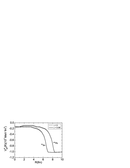
Figure 1: The Fermi average effective pairing interaction ${\cal V}^{\rm F}_{\rm eff}(R)$ for ¹²⁰Sn and ²⁰⁰Pb nuclei

The “experimental” gap value $\Delta_{\rm exp}$ for semi-magic nuclei is usually identified with a half of one of the following odd-even double mass differences (DMD):

$$D_{2n}^{+}(N,Z)=M(N+2,Z)+M(N,Z)-2M(N+1,Z),$$ (1)

$$D_{2n}^{-}(N,Z)=-M(N-2,Z)-M(N,Z)+2M(N-1,Z),$$ (2)

$$D_{2p}^{+}(N,Z)=M(N,Z+2)+M(N,Z)-2M(N,Z+1),$$ (3)

$$D_{2p}^{-}(N,Z)=-M(N,Z-2)-M(N,Z)+2M(N,Z-1).$$ (4)

The accuracy of such a prescription was estimated in Pankr2 as ${\simeq}0.1\div 0.2\;$MeV. Approximately the same accuracy holds for the “developed pairing” approximation in the gap equation, with conservation of the particle number only on average part-numb , used in all References on the pairing problem cited above.

There is one more physical quantity in semi-magic nuclei which can be evaluated in terms of the same effective interaction as the pairing gap. This is the set of the same double odd-even mass differences (1)–(4), but for the non-superfluid subsystems. Now $N$ is magic and $Z$ arbitrary in Eqs. (1),(2) and vice versa in Eqs. (3),(4). In non-superfluid nuclei, the mass differences, Eqs. (1),(2), coincide with poles in the total energy $E$ plane of the two-particle Green function $K(1,2,3,4)$ for normal systems AB in the $nn$-channel, and Eqs. (3),(4), in the $pp$-channel. The equation for $K$ in the channel $S=0,L=0$ could be expressed in terms of the same EPI ${\cal V}_{\rm eff}$ as the pairing gap. This point was marked in the old paper Sap-Tr , where these differences for double-magic nuclei were analyzed within the theory of finite Fermi systems (TFFS) AB . In that article, the density dependent EPI was introduced for the first time and arguments were found in favor of of the surface dominance in this interaction.

It is worth to stress that this calculation of mass difference for the non-superfluid subsystem within the mean field theory is a more rigorous operation than its identification with the double gap $\Delta$ of the BCS scheme in the superfluid one. The first such calculations with the use of the semi-microscopic model for the effective pairing interaction with the same value $\gamma=0.06$ of the phenomenological parameter of the model, found previously in the pairing problem, were carried out recently for several semi-magic chains Gnezd1 ; Gnezd2 ; Gnezd3 .

In this work, we analyze corrections to the mean field theory of double odd-even mass differences due to particle-phonon coupling (PC) effects. Three PC effects are taken into account, the phonon induced interaction, the renormalization of the “ends” due to the $Z$-factor corresponding to the pole PC contribution to the nucleon mass operator and the change of the single-particle energies. In the latter case, the non-pole (so-called “tadpole”) diagram for the mass operator is taken into account in addition to the usual pole one. We limit ourselves with the double-magic nuclei where the perturbation theory on the PC vertex $g_{L}$ is usually valid.

II Brief formalism

II.1 The semi-microscopic model of the effective pairing interaction

To begin with, we describe briefly the semi-microscopic model of the EPI which will be used for finding the double odd-even mass differences in non-superfluid nuclei. The general many-body form of the equation for the pairing gap is as follows AB ,

$$\Delta={\cal U}GG^{s}\Delta,$$ (5)

where ${\cal U}$ is the $NN$-interaction block irreducible in the two-particle channel, and $G$ ($G^{s}$) is the one-particle Green function without (with) pairing. We consider the singlet, $S=0$ and $L=0$, pairing only. The isospin indices are omitted for brevity. A symbolic multiplication denotes the integration over energy and intermediate coordinates and summation over spin variables as well. In the Brueckner theory, first, the block ${\cal U}$ should be replaced with the free $NN$-potential ${\cal V}$, which does not depend on the energy. Second, simple quasi-particle Green functions $G$ and $G^{s}$ are used, i.e. those without PC corrections and so on. In the result, Eq. (5) coincides with the one of the BCS approximation and can be reduced to the form usual for the Bogolyubov method,

$$\Delta=-{\cal V}\varkappa\,,$$ (6)

where

$$\varkappa=\int\frac{d\varepsilon}{2\pi i}GG^{s}\Delta$$ (7)

is the anomalous density matrix.

As it was discussed in Introduction, Eq. (5) converges very slowly due to the short-range character of $NN$ potential. To overcome this problem, a two-step renormalization method of solving the gap equation in nuclei was used in Refs. Pankr1 ; Pankr2 ; Sap1 . The complete Hilbert space of the pairing problem $S$ is split in the model subspace $S_{0}$, that includes the single-particle states with energies less than a separation energy $E_{0}$, and the complementary one, $S^{\prime}$. The gap equation is solved in the model space:

$$\Delta={\cal V}_{\rm eff}GG^{s}\Delta|_{S_{0}},$$ (8)

with the EPI ${\cal V}_{\rm eff}$ instead of the block ${\cal V}$ in the BCS version of the original gap equation (5). It obeys the Bethe–Goldstone type equation in the subsidiary space,

$${\cal V}_{\rm eff}={\cal V}+{\cal V}GG{\cal V}_{\rm eff}|_{S^{\prime}}.$$ (9)

In this equation, the pairing effects can be neglected provided the model space is sufficiently large, $E_{0}\gg\Delta$. That is why we replaced the Green function $G^{s}$ for the superfluid system with its counterpart $G$ for the normal system. The problem of slow convergence has passed now to Eq. (9) for the EPI ${\cal V}_{\rm eff}({\bf r}_{1},{\bf r}_{2},{\bf r}_{3},{\bf r}_{4})$. To solve it, the LPA method is used as it was discussed in the Introduction. It turned out Rep that, with a very high accuracy, at each value of the average c.m. coordinate ${\bf R}=({\bf r}_{1}+{\bf r}_{2}+{\bf r}_{3}+{\bf r}_{4})/4$, one can use in Eq. (9) the formulae of the infinite system embedded into a constant potential well $U=U({\bf R})$. This significantly simplifies the equation for ${\cal V}_{\rm eff}$, in comparison with the initial equation for $\Delta$. As a result, the subspace $S^{\prime}$ can be chosen as large as necessary to achieve the convergence. Accuracy of LPA depends on the separation energy $E_{0}$. For finite nuclei, the value of $E_{0}{=}40\;$MeV guarantees the accuracy better than 0.01 MeV for the gap $\Delta$.

To avoid uncertainties of explicit consideration of corrections to the BCS scheme discussed above, the semi-microscopic model was suggested in Refs.Pankr1 ; Pankr2 ; Sap1 . In this model, a small phenomenological addendum to the EPI is introduced which embodies in an effective way all these corrections. The simplest ansatz for it was used:

$${\cal V}_{\rm eff}({\bf r}_{1},{\bf r}_{2},{\bf r}_{3},{\bf r}_{4})=V^{\rm BCS}_{\rm eff}({\bf r}_{1},{\bf r}_{2},{\bf r}_{3},{\bf r}_{4})+$$

$$\gamma C_{0}\frac{\rho(r_{1})}{\bar{\rho}(0)}\prod_{i=2}^{4}\delta({\bf r}_{1}-{\bf r}_{i}).$$ (10)

Here $\rho(r)$ is the density of nucleons of the kind under consideration, and $\gamma$ are dimensionless phenomenological parameters. To avoid any influence of the shell fluctuations in the value of ${\rho}(0)$, the average central density ${\bar{\rho}(0)}$ is used in the denominator of the additional term. It is averaged over the interval of $r{<}2\;$fm. The first, ab initio, term in the r.h.s. of Eq. (10) is the solution of Eq. (9) in the framework of the LPA method described above, with $m^{*}{=}m$ in the subspace $S^{\prime}$.

II.2 Double mass differences in magic nuclei

As it is was discussed in Introduction, the double odd-even mass differences (1)–(4) in non-superfluid nuclei can be expressed in terms of the same EPI (9) as the gap (8). To derive the equation for this quantity, it is convenient to start from the Lehmann expansion for the two-particle Green function $K$ in a non-superfluid system. In the single-particle wave functions $|1\rangle{=}|n_{1},l_{1},j_{1},m_{1}\rangle$ representation, it reads AB :

$$K_{12}^{34}(E)=\sum_{s}\frac{\chi^{s}_{12}\chi^{s+}_{34}}{E-E_{s}^{+,-}\pm i\gamma},$$ (11)

where $E$ is the total energy in the two-particle channel and $E_{s}^{+,-}$ denote the eigen-energies of nuclei with two particles and two holes, respectively, added to the original nucleus. They are often interpreted as the “pair vibrations” BM2 . Instead of the Green function $K$, it is convenient to use the two-particle interaction amplitude $\Gamma$:

$$K=K_{0}+K_{0}\Gamma K_{0},$$ (12)

where $K_{0}=GG$. The amplitude $\Gamma$ obeys the following equation AB :

$$\Gamma={\cal U}+{\cal U}GG\Gamma,$$ (13)

where ${\cal U}$ is the same irreducible interaction block as in Eq. (5). Again, within the Brueckner theory, the block ${\cal U}$ should be replaced with the realistic $NN$-potential ${\cal V}$ which does not depend on the energy. Then the integration over the relative energy can be readily carried out in Eq. (13):

$$A_{12}{=}\int\frac{d\varepsilon}{2\pi i}G_{1}\left(\frac{E}{2}{+}\varepsilon\right)G_{2}\left(\frac{E}{2}{-}\varepsilon\right){=}\frac{1{-}n_{1}{-}n_{2}}{E{-}\varepsilon_{1}{-}\varepsilon_{2}},$$ (14)

where $\varepsilon_{1,2}$ are the single-particle energies and $n_{1,2}{=}(0;1)$, the corresponding occupation numbers. As the result, we obtain:

$$\Gamma={\cal V}+{\cal V}A\Gamma.$$ (15)

In vicinity of a pole $E{=}E_{s}$, one gets

$$\Gamma=\frac{d_{s}d_{s}^{+}}{E-E_{s}},$$ (16)

where $d_{s}^{+}\;(d_{s})$ are vertices of creation (anihillation) of the two-particle state $|s\rangle$, the non-homogeneous Eq. (15) reduces to the homogeneous one,

$$\Gamma={\cal V}A\Gamma,$$ (17)

which is, in fact, the in-medium Bethe-Salpeter equation, or equivalently

$$d_{s}={\cal V}Ad_{s},$$ (18)

.

It is more convenient to transform this equation to the one for the eigenfunctions $\chi^{s}=Ad_{s}$:

$$(E_{s}-\varepsilon_{1}-\varepsilon_{2})\chi^{s}_{12}=(1-n_{1}-n_{2})\sum_{34}{\cal V}_{12}^{34}\chi^{s}_{34}.$$ (19)

It is different from the Shrödinger equation for two interacting particles in an external field only with the factor $(1-n_{1}-n_{2})$ which reflects the many-body character of the problem, in particular, the Pauli principle. As in the pairing problem, the angular momenta of two-particle states $|12\rangle$, $|34\rangle$ are coupled to the total angular momentum $I{=}0$ ($S{=}0,L{=}0$).

The direct solution of this equation is complicated by the same reasons as for the ab initio BCS gap equation described above. The same two-step method is used in combination with LPA to overcome this difficulty. The usual renormalization of Eq. (19) transforms it into the analogous equation in the model space:

$$(E_{s}{-}\varepsilon_{1}{-}\varepsilon_{2})\chi^{s}_{12}{=}(1{-}n_{1}{-}n_{2}){\sum_{34}}^{0}\left({\cal V}_{\rm eff}\right)_{12}^{34}\;\chi^{s}_{34},$$ (20)

where the effective interaction ${\cal V}_{\rm eff}$ coincides with that of pairing problem, Eq. (9), provided the same value of the separation energy $E_{0}$ is used. It agrees with the well-known theorem by Thouless Thouless stating that the gap equation reduces to the in-medium Bethe-Salpeter equation provided the gap $\Delta$ vanishes. The next step consists in the use of the ansatz (10) to take into account corrections to the Brueckner theory with a phenomenological addendum ($\sim\gamma$).

The double mass differences (1)–(4) are identified with the two first solutions $E_{s}^{+,-}$ of Eq. (20), corresponding to the addition of two particles (holes) to the magic core into the state $\varepsilon_{1}=\varepsilon_{2}=\mu^{+,-}$, where the chemical potentials $\mu^{+,-}$ are defined in a usual way as mass differences, e.g., $\mu_{p}^{+}=E_{\rm B}(N,Z+1)-E_{\rm B}(N,Z)$. Then, the energy difference in the left-hand side of Eq. (20) is equal directly the quantity we need: $E_{s}^{+,-}-2\mu^{+,-}=D^{+,-}$.

In Refs. Gnezd1 ; Gnezd2 ; Gnezd3 this scheme of finding the DMD $D^{+,-}$ in non-superfluid systems within the semi-microscopic model was used for several chains of semi-magic nuclei. The proton subsystem should be considered for isotopic chains with magic $Z$ value and the neutron one, for isotonic chains where $N$ is magic. Reasonable results were obtained with the same value $\gamma{=}0.06$ which was previously found for the pairing gap Pankr2 . In this work, we study in an explicit form the PC effects in this problem and analyze possibility of modifying the optimal value of the parameter $\gamma$. This can be expected, since the PC effect was implicitly included in $\gamma$.

II.3 Particle-phonon coupling contributions to double mass differences

Introducing of the PC corrections to Eq. (20) consists, first, of the change of $\varepsilon_{\lambda}$ on the l.h.s. to $\widetilde{\varepsilon}_{\lambda}{=}\varepsilon_{\lambda}{+}\delta\varepsilon_{\lambda}^{\rm PC}$ and, second, a similar change of the ${\cal V}_{\rm eff}$ quantity on the r.h.s., to $\widetilde{\cal V}_{\rm eff}$, with the same meaning of the “tilde” symbol. Let us write down this PC corrected equation explicitly:

$$(E_{s}{-}\widetilde{\varepsilon}_{1}{-}\widetilde{\varepsilon}_{2})\chi^{s}_{12}{=}(1{-}n_{1}{-}n_{2}){\sum_{34}}^{0}\left(\widetilde{\cal V}_{\rm eff}\right)_{12}^{34}\;\chi^{s}_{34},$$ (21)

Let us begin with more transparent part of the problem concerning the single-particle energies. We follow here the method developed in levels . Note also that recently PC corrections to the single-particle energies within different self-consistent approaches were studied in Refs. Litv-Ring ; Bort ; Dobaczewski ; Baldo-PC .

To find the single-particle energies with account for the PC effects, we solve the following equation:

$$\left(\varepsilon-H_{0}-\delta\Sigma^{\rm PC}(\varepsilon)\right)\phi=0,$$ (22)

where $H_{0}$ is the quasiparticle Hamiltonian with the spectrum $\varepsilon_{\lambda}^{(0)}$ and $\delta\Sigma^{\rm PC}$ is the PC correction to the quasiparticle mass operator. After expanding this term in the vicinity of $\varepsilon=\varepsilon_{\lambda}^{(0)}$ one finds

$$\varepsilon_{\lambda}=\varepsilon_{\lambda}^{(0)}+Z_{\lambda}^{\rm PC}\delta\Sigma^{\rm PC}_{\lambda\lambda}(\varepsilon_{\lambda}^{(0)}),$$ (23)

with obvious notation. Here $Z^{\rm PC}$ denotes the $Z$-factor due to the PC effects,

$$Z_{\lambda}^{\rm PC}=\left({1-\left(\frac{\partial\delta\Sigma^{\rm PC}(\varepsilon)}{\partial\varepsilon}\right)_{\varepsilon=\varepsilon_{\lambda}^{(0)}}}\right)^{-1}.$$ (24)

Expression (23) corresponds to the perturbation theory in the $\delta\Sigma$ operator with respect to $H_{0}$. In this article, we limit ourselves to magic nuclei where the so-called $g_{L}^{2}$-approximation, $g_{L}$ being the $L$-phonon creation amplitude, is, as a rule, valid. It is worth mentioning that Eq. (23) is more general, including, say, $g_{L}^{4}$ terms. In the case when several $L$-phonons are taken into account, the total PC variation of the mass operator in Eqs. (22)–(24) is just the sum:

$$\delta\Sigma^{\rm PC}=\sum_{L}\Sigma^{\rm PC}_{L}.$$ (25)

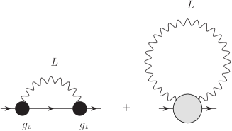
Figure 2: PC corrections to the mass operator. The gray blob denotes the “tadpole” term.

The diagrams for the $\delta\Sigma^{\rm PC}_{L}$ operator within the $g_{L}^{2}$-approximation are displayed in Fig. 2. The first one is the usual pole diagram, with obvious notation, whereas the second, “tadpole” diagram represents the sum of all non-pole diagrams of the $g_{L}^{2}$ order. For the pole term we are here neglecting the correction due to the one “bubble” diagram Baldo-PC . This can be justified provided only collective phonons are included. In the case of phonons of smaller collectivity, as e.g. positive parity states in ²⁰⁸Pb, this correction could be important.

In the obvious symbolic notation, the pole diagram corresponds to $\delta\Sigma^{\rm pole}=(g_{L},D_{L}Gg_{L})$ where $D_{L}(\omega)$ is the phonon $D$-function. Explicit expression for the pole term is well known, but we present it for completeness:

$$\delta\Sigma^{\rm pole}_{\lambda\lambda}(\epsilon) = \sum_{\lambda_{1}\,M}|\langle\lambda_{1}|g_{LM}|\lambda\rangle|^{2}$$ (26)

$$\times \left(\frac{n_{\lambda_{1}}}{\varepsilon+\omega_{L}-\varepsilon_{\lambda_{1}}}+\frac{1-n_{\lambda_{1}}}{\varepsilon-\omega_{L}-\varepsilon_{\lambda_{1}}}\right),$$

where $\omega_{L}$ is the excitation energy of the $L$-phonon. The $Z^{\rm PC}$-factor (24) can be easily found from (26) by finding the derivative over the energy $\varepsilon$.

The vertex $g_{L}$ obeys the TFFS RPA-like equation AB ,

$${g_{L}}(\omega)={{\cal F}}A_{\rm ph}(\omega){g_{L}}(\omega),$$ (27)

where ${\cal F}$ is the Landau–Migdal (LM) interaction amplitude, and $A_{\rm ph}(\omega)=\int G\left(\varepsilon+\omega/2\right)G\left(\varepsilon-\omega/2\right)d\varepsilon/(2\pi i)$ is the particle-hole propagator. It is normalized as follows AB :

$$\left(g_{L}^{+}\frac{dA_{\rm ph}}{d\omega}g_{L}\right)_{\omega=\omega_{L}}=-1,$$ (28)

with obvious notation.

We use the self-consistent scheme to solve Eq. (27) within the EDF method with the energy functional

$$E_{0}=\int{\cal E}[\rho_{n}({\bf r}),\rho_{p}({\bf r})]d^{3}r,$$ (29)

where ${\cal E}$ is the energy density. In this approach, the LM amplitude is found as the second variation derivative,

$${\cal F}_{\tau\tau^{\prime}}=\frac{\delta^{2}{E_{0}}}{\delta\rho_{\tau}\delta\rho_{\tau^{\prime}}},$$ (30)

$\tau{=}n,p$ being the isotopic index. The Fayans EDF we deal depends not only on the normal densities $\rho_{\tau}$ but on their anomalous counterparts $\nu_{\tau}$ as well. However, we deal now with magic nuclei where the anomalous densities vanish and we use therefore a simplified form (29) for $E_{0}$.

All the low-lying phonons we consider have natural parity. In this case, the vertex $g_{L}$ possesses even $T$-parity. It is a sum of two components with spins $S=0$ and $S=1$, respectively,

$$g_{L}=g_{L0}(r)T_{LL0}({\bf n,\alpha})+g_{L1}(r)T_{LL1}({\bf n,\alpha}),$$ (31)

where $T_{JLS}$ stand for the usual spin-angular tensor operators BM1 . The operators $T_{LL0}$ and $T_{LL1}$ have opposite $T$-parities, hence the spin component should be the odd function of the excitation energy, $g_{L1}\propto\omega_{L}$. This is the main reason why the $S=0$ component dominates in such states. It is demonstrated in Fig. 3 for $3^{-}_{1}$ state in ²⁰⁸Pb, where the $S=1$ components are multiplied by the factor 10 to be distinguishable.

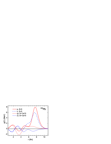
Figure 3: The vertex $g_{L}$ for the $3^{-}_{1}$ state in ²⁰⁸Pb.

A method to find the tadpole term for low-lying surface phonons was developed by Khodel Khod and is described in detail in KhS . It is equal to

$$\delta\Sigma^{\rm tad}=\int\frac{d\omega}{2\pi i}\delta_{L}{g_{L}}D_{L}(\omega),$$ (32)

where $\delta_{L}{g_{L}}$ can be found by variation of Eq. (27) in the field of the $L$-phonon:

$$\delta_{L}{g_{L}} = \delta_{L}{\cal F}A_{\rm ph}(\omega_{L}){g_{L}}+{\cal F}\delta_{L}A_{\rm ph}(\omega_{L}){g_{L}}$$ (33)

$$+ {\cal F}A_{\rm ph}(\omega_{L})\delta_{L}{g_{L}}.$$

The phonon $D$-function appears in Eq. (32) after connecting two wavy $L$-phonon ends in Eq. (33). This corresponds to averaging of the product of two boson (phonon) operators $B_{L}^{+}B_{L}$ over the ground state of the nucleus with no phonons.

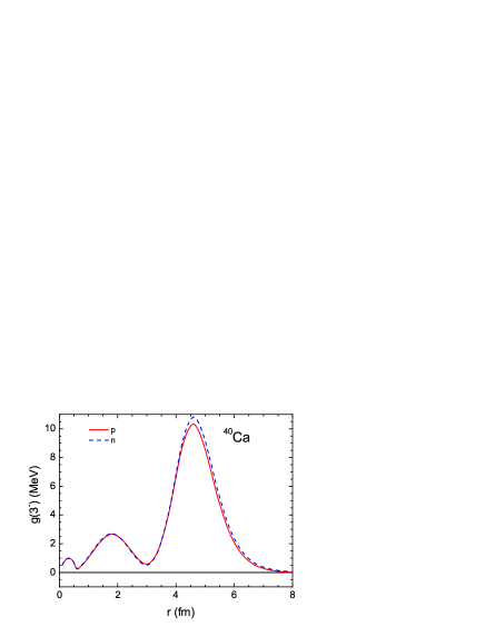
Figure 4: The vertex $g_{L}$ for the $3^{-}_{1}$ state in ⁴⁰Ca.

Following Ref. levels , we use an approximate way to solve Eq. (33) based on the surface dominance in the vertex $g_{L}({\bf r})$. Indeed, all the $L$-phonons we consider are the surface vibrations which belong to the Goldstone mode corresponding to the spontaneous breaking of the translation symmetry in nuclei Khod ; KhS . For the ghost phonon, $L{=}1,\omega_{1}{=}0$, which is the lowest energy member of this mode, Eq. (27), due to the TFFS self-consistency relation Fay-Khod , has the exact solution

$$g_{1}({\bf r})=\alpha_{1}\frac{dU(r)}{dr}Y_{1M}({\bf n}),$$ (34)

where $\alpha_{1}=1/\sqrt{2\omega B_{1}}$ , $B_{1}=3mA/4\pi$ is the Bohr–Mottelson (BM) mass coefficient BM2 and $U(r)$ is the central part of the mean-field potential generated by the energy functional.

In the general case, the coordinate form of the amplitude $g_{L}({\bf r})$ is very close to that of the ghost phonon:

$$g_{L}(r)=\alpha_{L}\frac{dU}{dr}+\chi_{L}(r),$$ (35)

where the in-volume correction $\chi_{L}(r)$ is rather small. The first, surface term on the right-hand sight. of Eq. (35) corresponds to the BM model for the surface vibrations BM2 , the amplitude $\alpha_{L}$ being related to the dimensionless BM amplitude $\beta_{L}$ as follows: $\alpha_{L}=R\beta_{L}/\sqrt{2L+1}$, where $R=r_{0}A^{1/3}$ is the nucleus radius, and $r_{0}=1.2\;$fm.

Fig. 3 demonstrates the smallness of the in-volume term of $g_{L}({\bf r})$ in the case of the $3^{-}_{1}$-state in ²⁰⁸Pb which is the most collective state in this nucleus. In more light nuclei, as ^40,48Ca, the surface dominance is not so pronounced but also persists. It is shown in Fig. 4 for the $3^{-}_{1}$ state in ⁴⁰Ca. If one neglects in-volume contributions, the tadpole PC term (32) can be reduced to a simple form:

$$\delta\Sigma^{\rm tad}_{L}=\frac{\alpha_{L}^{2}}{2}\frac{2L+1}{3}\triangle U(r).$$ (36)

It should be noted that this relation for the ghost phonon is exact. Below we neglect the in-volume corrections for all nuclei considered. To find the phonon amplitudes $\alpha_{L}$, we used the following definition

$$\alpha_{L}^{\tau}=\frac{g_{L}^{\tau,{\rm max}}}{\left(\frac{dU}{dr}\right)^{\tau,{\rm max}}},$$ (37)

with obvious notation.

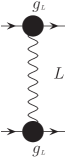
Figure 5: The phonon induced interaction.

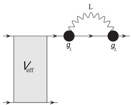
Figure 6: An example of the PC “end” correction.

Note that the above scheme for the ghost $L=1$ phonon results in an explicit expression for the “recoil effect”. Details can be found in levels .

Let us go to PC corrections to the r.h.s. of Eq. (20). They include the phonon induced interaction, Fig. 5, and the “end corrections”. An example of them is given in Fig. 6. Partial summing of such diagrams results in the “renormalization” of ends:

$$|\lambda\rangle\to|\widetilde{\lambda}\rangle=\sqrt{Z_{\lambda}^{\rm PC}}|\lambda\rangle.$$ (38)

In the result, we get

$$\langle 11^{\prime}|\widetilde{\cal V}_{\rm eff}|22^{\prime}\rangle = \sqrt{Z_{1}^{\rm PC}Z_{1^{\prime}}^{\rm PC}Z_{2}^{\rm PC}Z_{2^{\prime}}^{\rm PC}}$$ (39)

$$\times \langle 11^{\prime}|{\cal V}_{\rm eff}+{\cal V}_{\rm ind}|22^{\prime}\rangle.$$

Remind that we deal with the channel with $I{=0},S{=0},L{=0}$. Hence, the states $i,i^{\prime}$ in (39) possess the same single-particle angular momenta, $j_{1}{=}j_{1^{\prime}},l_{1}{=}l_{1^{\prime}};j_{2}{=}j_{2^{\prime}},l_{2}{=}l_{2^{\prime}}$. In this case, the explicit expression of the matrix element of ${\cal V}_{\rm ind}$ is as follows:

$$\langle 11^{\prime}|{\cal V}_{\rm ind}|22^{\prime}\rangle=-\frac{2\omega_{L}}{\sqrt{(2j_{1}+1)(2j_{2}+1)}}$$

$$\times\frac{\bigl{(}\langle j_{1}l_{1}||Y_{L}||j_{1}l_{1}\rangle(g_{L})_{11^{\prime}}\bigr{)}\bigl{(}\langle j_{2}l_{2}||Y_{L}||j_{2}l_{2}\rangle(g_{L})_{22^{\prime}}\bigr{)}^{*}}{\omega_{L}^{2}-(\varepsilon_{2}-\varepsilon_{1})^{2}},$$ (40)

where $\langle\;||Y_{L}||\;\rangle$ stands for the reduced matrix element BM1 , and $(g_{L})_{ii^{\prime}}$ are the radial matrix elements of the vertex $g_{L}(r)$. For brevity, we show here explicitly the contribution of the main term of Eq. (31) only, with $S{=}0$, $T_{LL0}=Y_{LM}({\bf n})\times\hat{1}$. In actual calculations, the component $S{=}1$ is also taken into account but its contribution is always small.

Table 1: Characteristics of the low-lying phonons in magic nuclei, $\omega_{L}$ (MeV) and $B(EL,{\rm up)}$(${\rm e^{2}fm}^{2L}$).

$L^{\pi}$	$\omega_{L}^{\rm th}$	$\omega_{L}^{\rm exp}$	$B(EL)^{\rm th}$	$B(EL)^{\rm exp}$
		$\qquad\qquad{}^{40}$Ca
$3^{-}$	3.335	3.73669 (5)	$1.52\times 10^{4}$	$1.24\times 10^{4}$
		$\qquad\qquad{}^{48}$Ca
$2^{+}$	3.576	3.83172 (6)	$0.55\times 10^{2}$	$0.86\times 10^{2}$
$3^{-}$	4.924	4.50678 (5)	$5.701\times 10^{3}$	$0.67\times 10^{4}$
		$\qquad\qquad{}^{56}$Ni
$2^{+}$	2.826	2.7006 (7)	$5.725\times 10^{2}$
$3^{-}$	8.108	4.932 (3)	$2.068\times 10^{4}$
		$\qquad\qquad{}^{78}$Ni
$2^{+}$	3.238	-	$3.309\times 10^{2}$
$3^{-}$	6.378	-	$1.549\times 10^{4}$
		$\qquad\qquad{}^{100}$Sn
$2^{+}$	3.978	-	$1.375\times 10^{3}$
$3^{-}$	5.621	-	$1.24\times 10^{5}$
		$\qquad\qquad{}^{132}$Sn
$2^{+}$	4.327	4.04120 (15)	$0.104\times 10^{4}$	$0.11(0.03)\times 10^{4}$
$3^{-}$	4.572	4.35194 (14)	$1.29\times 10^{5}$
		$\qquad\qquad{}^{208}$Pb
$3^{-}$	2.684	2.615	$7.093\times 10^{5}$	$6.12\times 10^{5}$
$5^{-}_{1}$	3.353	3.198	$3.003\times 10^{8}$	$4.47\times 10^{8}$
$5^{-}_{2}$	3.787	3.708	$1.785\times 10^{8}$	$2.41\times 10^{8}$
$2^{+}_{1}$	4.747	4.086	$1.886\times 10^{3}$	$3.18\times 10^{3}$
$2^{+}_{2}$	5.004	4.928	$1.148\times 10^{3}$	-
$4^{+}_{1}$	4.716	4.324	$3.007\times 10^{6}$	-
$4^{+}_{2}$	5.367	4.911(?)	$8.462\times 10^{6}$	-
$6^{+}_{1}$	4.735	-	$6.082\times 10^{9}$	-
$6^{+}_{2}$	5.429	-	$1.744\times 10^{10}$	-

Table 2: Different PC corrections to odd-even double mass differences of magic nuclei.

		$D_{2}^{(0)}$	$\delta D_{2}(Z^{\rm PC})$	$\delta D_{2}({\cal V}_{\rm ind}^{\rm PC})$	$\delta D_{2}(\delta\varepsilon^{\rm PC})$	$\delta D_{2}^{\rm PC}\;$	$D_{2}^{\rm PC}$	$D_{2}^{\rm exp}$
40Ca-pp	$D_{2}^{-}$	3.001	-0.427	-0.539	-0.206	-0.866	2.135	1.94683(19)
	$D_{2}^{+}$	-2.718	0.399	0.548	0.158	0.818	-1.900	-2.66622(28)
40Ca-nn	$D_{2}^{-}$	4.064	-0.911	-0.971	-0.357	-1.454	2.610	2.3395(9)
	$D_{2}^{+}$	-3.836	0.933	0.998	0.292	1.461	-2.375	-3.11785(15)
48Ca-pp	$D_{2}^{-}$	2.738	-0.762	0.071	0.184	-0.663	2.075	2.592(40)
	$D_{2}^{+}$	-3.047	0.908	-0.396	-0.280	0.449	-2.598	-2.5333(38)
48Ca-nn	$D_{2}^{-}$	3.079	-0.589	0.004	0.943	-0.286	2.793	2.6763(23)
	$D_{2}^{+}$	-1.715	0.344	0.096	-0.833	0.210	-1.505	-1.2141(16)
56Ni-pp	$D_{2}^{-}$	2.679	-0.577	0.245	0.148	-0.376	2.303	2.1022(4)
	$D_{2}^{+}$	-1.461	0.466	-0.512	-0.133	0.142	-1.319	-1.590(50)
56Ni-nn	$D_{2}^{-}$	3.092	-1.035	1.271	0.197	-0.787	2.305	2.5517(8)
	$D_{2}^{+}$	-1.931	0.617	-2.754	-0.201	0.413	-1.518	-1.9687(7)
78Ni-pp	$D_{2}^{-}$	4.161	-1.913	0.619	0.343	-1.558	2.603	-
	$D_{2}^{+}$	-3.525	1.873	-1.133	-0.120	1.415	-2.110	-1.980(980)#
78Ni-nn	$D_{2}^{-}$	2.330	-0.614	0.427	0.116	-0.221	2.109	2.240(1190)#
	$D_{2}^{+}$	-1.373	0.365	-0.305	-0.179	-0.012	-1.385	-
100Sn-pp	$D_{2}^{-}$	2.209	-0.595	0.338	0.035	-0.282	1.927	2.170(410)#
	$D_{2}^{+}$	-1.190	0.306	-0.133	0.022	0.188	-1.002	-
100Sn-nn	$D_{2}^{-}$	2.651	-0.737	0.363	0.075	-0.418	2.233	-
	$D_{2}^{+}$	-1.652	0.462	-0.138	-0.011	0.331	-1.321	-1.610(540)
132Sn-pp	$D_{2}^{-}$	3.184	-1.506	-0.015	-0.982	-1.198	1.986	2.027(160)
	$D_{2}^{+}$	-2.763	1.319	-0.250	1.710	1.494	-1.269	-1.234(6)
132Sn-nn	$D_{2}^{-}$	2.301	-0.396	0.369	-0.009	-0.161	2.140	2.132(9)
	$D_{2}^{+}$	-1.165	0.217	-0.102	-0.045	0.094	-1.071	-1.227(6)
208Pb-pp	$D_{2}^{-}$	1.680	-0.824	-0.083	0.569	-0.745	0.935	0.627(22)
	$D_{2}^{-}$	-2.286	1.049	-0.167	-0.329	0.830	-1.456	-1.1845(11)
208Pb-nn	$D_{2}^{-}$	0.778	-0.275	0.174	0.205	-0.113	0.665	0.63009(11)
	$D_{2}^{-}$	-1.156	0.443	-0.691	-0.021	0.165	-0.991	-1.2478(17)

Table 3: PC contributions to the SP characterisics of ground states $\lambda_{0}$ of odd neighbors of magic nuclei.

nucleus	$\lambda_{0}$	$\varepsilon^{(0)}_{\lambda_{0}}$	$\delta\varepsilon_{\lambda_{0}}^{\rm PC}$	$Z^{\rm PC}_{\lambda_{0}}$
40Ca	$1f_{7/2}^{p}$	-2.678	0.479	0.960
	$1d_{3/2}^{-p}$	-7.265	0.122	0.966
	$1f_{7/2}^{n}$	-9.593	0.270	0.947
	$1d_{3/2}^{-n}$	-14.257	0.076	0.965
48Ca	$1f_{7/2}^{p}$	-9.909	-0.031	0.899
	$2s_{1/2}^{-p}$	-15.098	0.575	0.916
	$2p_{3/2}^{n}$	-5.784	-0.062	0.940
	$1f_{7/2}^{-n}$	-9.488	0.357	0.966
56Ni	$2p_{3/2}^{p}$	-1.905	-0.151	0.913
	$1f_{7/2}^{-p}$	-6.276	0.530	0.963
	$2p_{3/2}^{n}$	-11.064	-0.074	0.934
	$1f_{7/2}^{-n}$	-15.588	0.486	0.945
78Ni	$2p_{3/2}^{p}$	-15.526	-0.154	0.882
	$1f_{7/2}^{-p}$	-20.245	0.491	0.943
	$2d_{5/2}^{n}$	-1.477	-0.137	0.916
	$1g_{9/2}^{-n}$	-5.481	0.460	0.918
100Sn	$2d_{5/2}^{p}$	2.812	-0.214	0.910
	$1g_{9/2}^{-p}$	-2.345	0.492	0.939
	$2d_{5/2}^{n}$	-11.180	-0.194	0.901
	$1g_{9/2}^{-n}$	-16.449	0.511	0.939
132Sn	$1g_{7/2}^{p}$	-9.892	0.227	0.967
	$1g_{9/2}^{-p}$	-14.842	0.363	0.963
	$2f_{7/2}^{n}$	-2.319	-0.131	0.939
	$1g_{9/2}^{-n}$	-7.472	0.376	0.948
208Pb	$1h_{9/2}^{p}$	-4.232	0.273	0.958
	$3s_{1/2}^{-p}$	-7.611	-0.023	0.930
	$2g_{9/2}^{n}$	-3.674	-0.251	0.885
	$3p_{1/2}^{-n}$	-7.506	-0.043	0.928

Table 4: Double odd-even mass differences of magic nuclei.

		$D_{2}^{(0)}$	$D_{2}(\gamma{=}0.06)$	$D_{2}^{\rm PC}$	$D_{2}^{\rm PC}(\gamma{=}0.06)$	$D_{2}^{\rm PC}(\gamma{=}0.03)$	$D_{2}^{\rm exp}$
40Ca-pp	$D_{2}^{-}$	3.001	2.391	2.424	2.038	2.217	1.94683(19)
	$D_{2}^{+}$	-2.718	-2.154	-2.202	-1.786	-1.987	-2.66622(28)
40Ca-nn	$D_{2}^{-}$	4.064	2.955	2.610	2.164	2.153	2.3395(9)
	$D_{2}^{+}$	-3.836	-2.773	-2.375	-1.959	-2.148	-3.11785(15)
48Ca-pp	$D_{2}^{-}$	2.738	2.109	2.075	1.708	1.879	2.592(40)
	$D_{2}^{+}$	-3.047	-2.394	-2.598	-2.203	-2.388	-2.5333(38)
48Ca-nn	$D_{2}^{-}$	3.079	2.441	2.793	2.282	2.518	2.6763(23)
	$D_{2}^{+}$	-1.715	-1.335	-1.505	-1.229	-1.353	-1.2141(16)
56Ni-pp	$D_{2}^{-}$	2.679	2.097	2.303	1.892	2.087	2.1022(4)
	$D_{2}^{+}$	-1.461	-1.107	-1.319	-1.098	-1.203	-1.590(50)
56Ni-nn	$D_{2}^{-}$	3.092	2.423	2.305	1.959	2.124	2.5517(8)
	$D_{2}^{+}$	-1.931	-1.484	-1.518	-1.278	-1.393	-1.9687(7)
78Ni-pp	$D_{2}^{-}$	4.161	2.835	2.603	2.120	2.341	-
	$D_{2}^{+}$	-3.525	-2.213	-2.110	-1.687	-1.878	-1.980(980)#
78Ni-nn	$D_{2}^{-}$	2.330	1.815	2.109	1.764	1.927	2.240(1190)#
	$D_{2}^{+}$	-1.373	-1.111	-1.385	-1.231	-1.302	-
100Sn-pp	$D_{2}^{-}$	2.209	1.710	1.927	1.599	1.754	2.170(410)#
	$D_{2}^{+}$	-1.190	-0.869	-1.002	-0.824	-0.907	-
100Sn-nn	$D_{2}^{-}$	2.651	2.032	2.233	1.837	2.023	-
	$D_{2}^{+}$	-1.652	-1.212	-1.321	-1.080	-1.191	-1.610(540)
132Sn-pp	$D_{2}^{-}$	3.184	2.281	1.986	1.812	1.905	2.027(160)
	$D_{2}^{+}$	-2.763	-1.875	-1.269	-1.444	-1.351	-1.234(6)
132Sn-nn	$D_{2}^{-}$	2.301	1.742	2.140	1.692	1.901	2.132(9)
	$D_{2}^{+}$	-1.165	-0.900	-1.071	-0.879	-0.967	-1.227(6)
208Pb-pp	$D_{2}^{-}$	1.680	1.000	0.935	0.718	0.815	0.627(22)
	$D_{2}^{+}$	-2.286	-1.467	-1.456	-1.120	-1.276	-1.1845(11)
208Pb-nn	$D_{2}^{-}$	0.778	0.530	0.665	0.494	0.570	0.63009(11)
	$D_{2}^{+}$	-1.156	-0.821	-0.991	-0.820	-0.899	-1.2478(17)

Table 5: Difference between theoretical and experimental values of DMD for different versions of the theory.

	$\gamma{=}0$	$\gamma{=}0.06$	$(\gamma{=}0)^{\rm PC}$	$(\gamma{=}0.06)^{\rm PC}$	$(\gamma{=}0.03)^{\rm PC}$	$D_{2}^{\rm exp}$
40Ca-pp	1.054	0.444	0.477	0.091	0.270	1.94683(19)
	-0.052	0.512	0.464	0.880	0.679	-2.66622(28)
40Ca-nn	1.724	0.615	0.270	-0.175	-0.187	2.3395(9)
	-0.718	0.345	0.743	1.159	0.970	-3.11785(15)
48Ca-pp	0.146	-0.483	-0.517	-0.884	-0.713	2.592(40)
	-0.514	0.139	-0.065	0.330	0.145	-2.5333(38)
48Ca-nn	0.403	-0.235	0.117	-0.394	-0.158	2.6763(23)
	-0.501	-0.121	-0.291	-0.015	-0.139	-1.2141(16)
56Ni-pp	0.577	-0.005	0.201	-0.210	-0.015	2.1022(4)
	0.129	0.483	0.271	0.492	0.387	-1.590(50)
56Ni-nn	0.540	-0.129	-0.247	-0.593	-0.428	2.5517(8)
	0.038	0.485	0.451	0.691	0.576	-1.9687(7)
132Sn-pp	-1.529	-0.641	-0.035	-0.210	-0.117	-1.234(6)
132Sn-nn	0.169	-0.390	0.008	-0.440	-0.231	2.132(9)
	0.062	0.327	0.156	0.348	0.260	-1.227(6)
208Pb-pp	1.053	0.373	0.308	0.091	0.188	0.627(22)
	-1.101	-0.282	-0.271	0.065	-0.091	-1.1845(11)
208Pb-nn	0.148	-0.100	0.035	-0.136	-0.060	0.63009(11)
	0.092	0.427	0.257	0.428	0.349	-1.2478(17)

III Calculation results

All calculations are carried out in a self-consistent way with the use of the Fayans EDF with the set DF3-a of the parameters Tol-Sap . We limit ourselves with seven double-magic nuclei, from ⁴⁰Ca till ²⁰⁸Pb. It should be noted that some of “new magic nuclei” are included into consideration just for completeness as corresponding experimental DMD are not known. Moreover, some nuclei necessary to find corresponding DMD from Eqs. (1)–(4) do not exist, being absolutely unstable; hence there is no hope that the corresponding experimental data will appear in future. This is so, e.g. with the ⁹⁸Sn nucleus which is a term of the DMD $D_{2}^{n-}(^{100}{\rm Sn})$ or ¹⁰¹Sb and ¹⁰²Te nuclei which are necessary to find the DMD $D_{2}^{n-}(^{100}{\rm Sn})$. Characteristics of the low-lying collective states in these nuclei are presented in Table 1. As one can see, the overall agreement of $\omega_{L}$ and $B(EL)$ values with known experimental data looks reasonable.

As it is well known, see e.g. levels , PC corrections are important mainly for single-particle states close to the Fermi surface. In practice, we solve the “PC corrected” equation (21) limiting ourselves with two shells nearby the Fermi level. In addition, we as a rule include into the calculation scheme the single-particle states of negative energy only. In Table 2, the effect of each PC correction to each DMD value is given separately. In this set of calculations we put $\gamma{=}0$ in Eq. (10) which determines the EPI of the semi-microscopic model, hence $D_{2}^{(0)}$ means the “ab initio” prediction for the DMD. The next columns present separate PC corrections to this quantity. So, the 2-nd column shows the result of application of Eq. (39) with ${\cal V}_{\rm ind}{=}0$, whereas the 3-rd one presents the effect of ${\cal V}_{\rm ind}$ itself with $Z_{1}^{\rm PC}{=}...{=}Z_{2^{\prime}}^{\rm PC}{=}1$. The column 4 shows the effect of PC corrections to the SP energies in Eq. (21) only. At last, column 5 presents the total PC effect $\delta D_{2}^{\rm PC}{=}D_{2}^{\rm PC}-D_{2}^{(0)}$, where $D_{2}^{\rm PC}$ (column 6) is the solution of Eq. (21) with all PC corrections included. As it should be, the value of $\delta D_{2}^{\rm PC}$ does not equal to the sum of the values in previous three columns because of an interference between different PC effects. Experimental DMD values are found from the mass table mass .

General impression from the analysis of Table 2 is that different PC corrections to DMD values are very non-regular, strongly depending on the nucleus under consideration and the two-particle channel as well. The $Z$-factor effect (column 2) always has the sign opposite to that of $D_{2}^{(0)}$ value thus suppressing the absolute value of $D_{2}^{(0)}$. This is a trivial consequence of the $Z^{\rm PC}<1$ condition. The scale of suppression varies from $\simeq 15$% (protons in ⁴⁰Ca) to $\simeq 50$% (protons in ¹³²Sn or ²⁰⁸Pb). The suppression value $\delta D_{2}({\cal V}_{\rm ind}^{\rm PC})$ is of the order of the product of $D_{2}^{(0)}(1{-}Z^{\rm PC}_{\lambda_{0}})^{2}$, where the $Z^{\rm PC}_{\lambda_{0}}$ value is given in Table 3. Here $\lambda_{0}$ denotes the single-particle state of a nucleon added to (or removed from) the magic nucleus under consideration. These two quantities should coincide if we use the “diagonal approximation” retaining in Eq. (21) the term $\lambda_{1}=\lambda_{2}=\lambda_{3}=\lambda_{4}=\lambda_{0}$ only. However, non-diagonal terms play some role in this equation making these two quantities equal only approximately.

The sign of the PC effect due to the induced interaction in the major part cases coincides with that of $D_{2}^{(0)}$, i.e. corresponds to an additional attraction. However, there are exceptions, e.g. ⁴⁰Ca nucleus, both proton and neutron modes. As a rule, the value of this effect is less than that of the $Z$-factors, but there are cases where it is rather big. This is so, e.g. in both neutron modes in ⁴⁰Ca. It occurs due to appearance of a small denominators in Eq. (40) corresponding to the states $\lambda_{2}{=}1f_{7/2}$ and $\lambda_{1}{=}1d_{2/2};2s_{1/2}$. This effect is even stronger in the neutron $D_{2}^{+}$ mode in ⁵⁶Ni due to the same SP states leading to small denominators in Eq. (40). Such cases of anomalously large value of the PC correction due to the induced interaction is a signal that the $g_{L}^{2}$ perturbation theory does not work sometimes even in magic nuclei and higher order $g_{L}^{2}$ terms should be taken into account. The use of the PC corrected single-particle energies in Eq. (40) is one of possible ways. Fortunately, this term in Eq. (39) for the neutron $D_{2}^{+}$ mode in ⁵⁶Ni is strongly suppressed with the $Z$-factors so that the resulting PC effect (column 5) turns out to be moderate. However, we are forced to interpret this result, just as those for the neutron modes in ⁴⁰Ca, as very approximate.

At last, go to the single-particle energy effect (column 4). In the “diagonal approximation” it should be equal to the double value of $\delta\varepsilon^{\rm PC}_{\lambda_{0}}$, see Table 3. As above $\lambda_{0}$ is the single-particle state of the odd nucleon, added to or removed from the double magic core. As it can be seen in the table, this quantity varies strongly depending on the nucleus and the state $\lambda_{0}$. However, again there is no complete coincidence between $\delta D_{2}(\delta\varepsilon^{\rm PC})$ and $\delta\varepsilon^{\rm PC}_{\lambda_{0}}$ values due to some effect of non-diagonal terms in Eq. (21). Moreover, sometimes these two quantities even have opposite signs, but always they are of the same order of magnitude. We did not show contributions to $\delta\varepsilon^{\rm PC}_{\lambda_{0}}$ of the pole and tadpole diagrams separately. It can be found in levels where it is shown that the tadpole term, as a rule, diminishes the value of $|\delta\varepsilon^{\rm PC}|$ at approximately $30-50$%. Partially due to this compensation, the single-particle energy effect is, as a rule, significantly less than two PC effects discussed previously. However, there is a case, both neutron modes in ⁴⁸Ca, where this PC effect dominates. Thus, all three PC effects under consideration should be taken into account on equal footing.

On average, account for PC effects makes agreement with experiment better, often significantly. However, there are several cases, the proton $D_{2}^{+}$ mode in ⁴⁰Ca and ⁵⁶Ni and the neutron $D_{2}^{+}$ mode in ⁵⁶Ni, where they make agreement worse.

In Table 4 we analyze together the PC effects considered above with the suppression of the EPI in the semi-microscopic model with non-zero value of the phenomenological parameter $\gamma$. Notation is similar to that in Table 2, i.e. the first two columns of Tables 2 and 4 coincide. Further, $D_{2}(\gamma{=}0.06)$ means the solution of Eq. (20) (i.e. that without PC effects) with $\gamma{=}0.06$ in Eq. (10). The column 3 of this table coincides with the column 6 of Table 2. Now, $D_{2}^{\rm PC}(\gamma{=}0.06)$ (column 4) and $D_{2}^{\rm PC}(\gamma{=}0.03)$ (column 5) mean the solutions of Eq. (21) with ${\cal V}_{\rm eff}$ in Eq. (39) found with $\gamma{=}0.06$ and $\gamma{=}0.03$, correspondingly. At first sight, PC corrections make agreement with the data better and the version of $D_{2}^{\rm PC}(\gamma{=}0.03)$ looks on average the best one among five theoretical columns. To make the comparison with experiment more transparent, we present in Table 5 differences between each of these theoretical prediction and the corresponding experimental value. 18 cases are chosen where the experimental data exist and possess sufficiently high accuracy. Let us concentrate mainly on comparison of the column of $(\gamma{=}0.03)^{\rm PC}$ with the one corresponding to $\gamma{=}0.06$ without PC corrections. The latter is a representative of the original semi-microscopic model without PC corrections with the optimal description of the pairing gap Pankr3; Sap1 and DMD of non-superfluid components of semi-magic nuclei Gnezd1 ; Gnezd2 ; Gnezd3 as well. The situation is essentially different for lighter nuclei, from ⁴⁰Ca till ⁵⁶Ni, and for heavier ones, beginning from ¹³²Sn. In the first case, the situation is “fifty-fifty”, i.e. approximately in a half of the cases PC corrections make agreement better and in a half, worse. Agreement typically becomes worse in the cases discussed above where the applicability of the perturbation theory for the induced interaction is questionable. Especially strong disagreement arises for the neutron $D_{2}^{+}$ mode in ⁴⁰Ca. Absolutely another situation takes place in the lower part of Table 5 for heavy nuclei. Here the PC corrections to DMD values taken into account make agreement better in all cases. Sometimes the improvement is significant, e.g. for the proton $D_{2}^{+}$ mode in ¹³²Sn and ²⁰⁸Pb nuclei.

IV Conclusion

A method is developed to account for the PC effects in the problem of finding odd-even DMD of magic nuclei within the ab initio approach starting from a realistic $NN$-potential. Recently, the semi-microscopic model of the EPI ${\cal V}_{\rm eff}$ developed first for the pairing problem Pankr1 ; Pankr2 ; Sap1 was applied to the odd-even DMD for non-superfluid subsystems of semi-magic nuclei Gnezd1 ; Gnezd2 ; Gnezd3 . The DMD values are found by solving the in-medium Bethe-Salpeter equation with the same EPI ${\cal V}_{\rm eff}$ as that in the pairing gap equation. The semi-microscopic model starts from the interaction ${\cal V}_{\rm eff}$ found in terms of a free $NN$-potential (Argonne $v_{18}$ in our case), the gap equation being solved in the basis with the bare mass $m^{*}{=}m$. Then the obtained EPI is supplemented with a phenomenological repulsive $\delta$-term proportional to a dimensionless parameter $\gamma$. The value of $\gamma{=}0.06$ found in Pankr2 to reproduce experimental gap values turned out to be also optimal for describing the DMD values in non-superfluid sub-systems Gnezd1 ; Gnezd2 ; Gnezd3 . The phenomenological addendum supposedly embodies on average three different corrections to the simple BCS scheme milan2 ; milan3 , the PC contribution, that from the effect of the effective mass $m^{*}{\neq}m$ and the one due to the high-lying excitations. The last two phenomena are presumably universal and their description with a universal parameter $\gamma$ looks reasonable. On the contrary, low-lying phonon characteristics vary significantly depending on the nucleus under consideration. Therefore, the PC contributions to the gap or the DMD values may fluctuate from nuclei to nuclei. In this work, we analyze the PC corrections to DMD values found within the semi-microscopic with possible change of the parameter $\gamma$.

We limit ourselves with seven magic nuclei, from ⁴⁰Ca till ²⁰⁸Pb. Three PC effects are taken into account, the phonon induced effective interaction, the “end” correction, and the change of the single-particle energies. The perturbation theory in $g^{2}_{L}$, where $g_{L}$ is the vertex of the $L$-phonon creation, is used. However, higher order in $g^{2}_{L}$ terms are included in the calculation scheme with partial summation of the end diagram. It results in a renormalization of the end single-particle wave functions, $|\lambda\rangle\to\sqrt{Z_{\lambda}^{\rm PC}}|\lambda\rangle$. PC corrections to single-particle energies are found self-consistently with an approximate account for the tadpole diagram. For lighter part of the set of magic nuclei, from ⁴⁰Ca till ⁵⁶Ni, the cases divide approximately in half between those where the PC corrections to DMD values make agreement with experiment better and the ones with the opposite result. In the major part of the “bad” cases, a poor applicability of the perturbation theory for the induced interaction, because of appearance of “dangerous” terms with small energy denominators, is the most probable reason of the disagreement. For intermediate nuclei, ⁷⁸Ni and ¹⁰⁰Sn, there is no sufficiently accurate data on their masses. Finally, for heavier nuclei, ¹³²Sn and ²⁰⁸Pb, PC corrections to DMD always make agreement with the experiment better. In this case, the optimal value of the phenomenological parameter of the semi-magic model reduces to $\gamma{=}0.03$. This result makes it promising a programme of systematic account for the PC corrections to the semi-microscopic model. There are two possible ways in this direction. The first one is consideration of a wider amount of nuclei, including semi-magic ones, but with more careful separation of cases with good applicability of the perturbation theory in $g^{2}_{L}$. The second one is an attempt to develop a more consistent theory with higher in $g^{2}_{L}$ terms for consideration of the dangerous terms. Both programs are now in progress.

- (1) F. Barranco, R. A. Broglia, H. Esbensen, and E. Vigezzi, Phys. Lett. B390, 13 (1997).
- (2) F. Barranco, R. A. Broglia, G. Colo, et al., Eur. Phys. J. A 21, 57 (2004).
- (3) A. Pastore, F. Barranco, R. A. Broglia, and E. Vigezzi, Phys. Rev. C 78, 024315 (2008).
- (4) E. Chabanat, P. Bonche, P. Haensel, J. Meyer, and R. Schaeffer, Nucl. Phys. A627, 710 (1997).
- (5) M. Baldo, U. Lombardo, S. S. Pankratov, E. E. Saperstein. J. Phys. G: Nucl. Phys., 37, 064016 (2010).
- (6) E. E. Saperstein, M. Baldo, in 50 Years of Nuclear BCS, World Scientific Review Volume, Editors R. Broglia and V. Zelevinsky (Singapure), Chapter 19 (p. 263-273) (2012).
- (7) T. Duguet and T. Lesinski, Eur. Phys. J. Special Topics 156, 207 (2008).
- (8) K. Hebeler, T. Duguet, T. Lesinski, and A. Schwenk, Phys. Rev. C 80, 044321 (2009).
- (9) S. K. Bogner, T. T. S. Kuo, and A. Schwenk, Phys. Rep. 386, 1 (2003).
- (10) L.-W. Siu, J. W. Holt, T. T. S. Kuo, and G. E. Brown, Phys. Rev. C 79, 054004 (2009).
- (11) S. S. Pankratov, M. Baldo, M. V. Zverev, U. Lombardo, E. E. Saperstein, S. V. Tolokonnikov, JETP Lett., 90, 612 (2009).
- (12) T. Duguet, in 50 Years of Nuclear BCS, World Scientific Review Volume, Editors R. Broglia and V. Zelevinsky (Singapure), Chapter 17 (p. 229-242) (2012).
- (13) E. Epelbaum, H.-W. Hammer and U.-G. Meissner, Rev. Mod. Phys. 81, 1773 (2009).
- (14) S. S. Pankratov, M. V. Zverev, M. Baldo, U. Lombardo, E. E. Saperstein, Phys. Rev. C 84, 014321 (2011).
- (15) E. E. Saperstein, M. Baldo, U. Lombardo, S. S. Pankratov, M. V. Zverev, Phys. Atom. Nucl., 74, 1644 (2011).
- (16) A. V. Smirnov, S. V. Tolokonnikov, S. A. Fayans, Sov. J. Nucl. Phys. 48, 995 (1988).
- (17) I. N. Borzov, S. A. Fayans, E. Krmer, and D. Zawischa, Z. Phys. A 335,117 (1996).
- (18) S. A. Fayans, JETP Lett. 68, 169 (1998).
- (19) S. A. Fayans, S.V. Tolokonnikov, E. L. Trykov, and D. Zawischa, Nucl. Phys. A676, 49 (2000).
- (20) S.V. Tolokonnikov and E. E. Saperstein, Phys. At. Nucl. 73, 1684 (2010).
- (21) S.V. Tolokonnikov, S. Kamerdzhiev, D. Voytenkov, S. Krewald, and E.E. Saperstein, arXiv:1107.2432v2[nucl-th], Phys. Rev. C 84, 064324 (2011).
- (22) M. Baldo, U. Lombardo, E.E. Saperstein, and M.V. Zverev Phys. Rep. 391, 261 (2004).
- (23) Abhishek Mukherjee, Y. Alhassid, and G. F. Bertsch, Phys. Rev. C 83, 014319 (2011).
- (24) A. B. Migdal Theory of finite Fermi systems and applications to atomic nuclei (Wiley, New York, 1967).
- (25) E. E. Saperstein, M. A. Troitsky, Yad. Fiz. 1, 400 (1965).
- (26) N. V. Gnezdilov, E. E. Saperstein, JETP Lett, 95, 603 (2012).
- (27) E. E. Saperstein, M. Baldo, N. V. Gnezdilov, U. Lombardo and S. S. Pankratov EPJ Web of Conferences 38, 05002 (2012).
- (28) N. V. Gnezdilov, E. E. Saperstein, Phys. At. Nucl. 77, 185 (2014).
- (29) A. Bohr and B. R. Mottelson, Nuclear Structure (Benjamin, New York, Amsterdam, 1974.), Vol. 2.
- (30) D. J. Thouless, Ann. Phys. 10, 553 (1960).
- (31) N. V. Gnezdilov, I. N. Borzov, E. E. Saperstein, and S. V. Tolokonnikov, Phys. Rev. C 89, 034304 (2014).
- (32) E. Litvinova and P. Ring, Phys. Rev. C 73, 044328 (2006).
- (33) Li-Gang Cao, G. Colò, H. Sagawa, and P. F. Bortignon, Phys. Rev. C 89, 044314 (2014).
- (34) D. Tarpanov, J. Dobaczewski, J. Toivanen, and B. G. Carlsson, Phys. Rev. Lett. 113, 252501 (2014).
- (35) M. Baldo, P. F. Bortignon, G. Coló, D. Rizzo, and L. Sciacchitano, J. Phys. G: Nucl. Phys. 42, 085109 (2015).
- (36) A. Bohr and B.R. Mottelson, Nuclear Structure (Benjamin, New York, Amsterdam, 1969.), Vol. 1.
- (37) V. A. Khodel, JETP Lett. 16, 291 (1972)]; ,18, 126 (1973); Sov. J. Nucl. Phys. 19, 376 (1974).
- (38) V. A. Khodel and E. E. Saperstein, Phys. Rep. 92, 183 (1982).
- (39) S. A. Fayans and V. A. Khodel, JETP Lett. 17, 444 (1973).
- (40) M. Wang, G. Audi, A. H. Wapstra, F. G. Kondev, M. MacCormick, X. Xu, and B. Pfeiffer, Chinese Physics C, 36, 1603 (2012).