A sufficient set of experimentally implementable thermal operations

Abstract

Recent work using tools from quantum information theory has shown that at the nanoscale where quantum effects become prevalent, there is not one thermodynamical second law but many. Derivations of these laws assume that an experimenter has very precise control of the system and heat bath. Here we show that these multitude of laws can be saturated using two very simple operations: changing the energy levels of the system and thermalizing over any two system energy levels. Using these two operations, one can distill the optimal amount of work from a system, as well as perform the reverse formation process. Even more surprisingly, using only these two operations and one ancilla qubit in a thermal state, one can transform any state into any other state allowable by the second laws. We thus have the remarkable result that the second laws hold for fine-grained manipulation of system and bath, but can be achieved using very coarse control. This brings the full array of thermal operations into a regime accessible by experiment, and establishes the physical relevance of these second laws.

I Introduction

Thermodynamics and statistical physics are one of the most successful areas of physics, owing to its broad applicability. One can make statements which do not depend on the particulars of the dynamics, and such laws govern much of the world around us. Thermodynamics puts limitations on the efficiency of our cars’ engines, determines the weather, can be used to predict many phenomena in particle accelerators, and even plays a central role in areas of fundamental physics, providing one of the only clues we have to a quantum theory of gravity through the laws of black hole thermodynamics. However, traditional thermodynamics, as derived from statistical mechanics, generally concerns itself with the average behavior of large systems, composed of many particles. Here the experimenter is only able to manipulate macroscopic quantities of the material such as its pressure and volume, and does not have access to the microscopic degrees of freedom of the system, much less the heat bath. The basic operations are limited to very crude control of the system-bath – isotherms, adiabats, isochors etc.

However, as our abilities to manipulate and control small thermodynamical systems improve, we are able to control the microscopic degrees of freedom of smaller and smaller systems Scovil and Schulz-DuBois (1959); Scully (2002); Rousselet et al. (1994); Faucheux et al. (1995); Baugh et al. (2005). It thus seems natural to consider the thermodynamical behavior of small, finite sized systems or heat engines composed of just a few molecules.

For a $d$-level system interacting with a heat bath, one can imagine an experimenter manipulating the system, who has control over each of the levels and can interact the system in any way they want with the heat bath. From a practical point of view, needing to perform such arbitrary interactions is undesirable as they require very precise control over and be able to keep track of the entirety of the heat bath. Simpler interactions would be much more appealing. See Figure 1 for a schematic of this comparison.

However, even if one allows for such fine-grained control, the most experimentally unfeasible scenario, the second law of thermodynamics still holds (provided one computes the entropy of the system in terms of its microstates rather than using a course grained entropy). In fact, not only does the traditional second law hold, but additional second laws emerge at the nano-scale such as the so-called thermo-majorization criteria Ruch and Mead (1976); Horodecki and Oppenheim (2013), and those given by a family of generalized free energies Brandao et al. (2015) . These constrain the set of states it is possible to transition to from a given starting state and converge to the familiar second law in the thermodynamic limit.

However, such precise control will be impossible to implement as it could require accurately manipulating all of the $10^{20}$ molecules contained in a typical heat bath. As such, it may seem what an experimenter can achieve without such incredibly fine-grained control must be very far from what is allowed by the second laws Wilming et al. (2014). This contrasts sharply with traditional, macroscopic thermodynamics. There, those transformations allowed by the standard second law can easily be achieved by controlling macroscopic, coarse-grained parameters such as a system’s volume or an external field. If the same level of control was needed macroscopically as seems necessary at the nano-scale, then running a car efficiently would require control of all of the molecules in the exploding fuel and cooler. Clearly this would be an undesirable feature - must it exist at the nano-scale? The existence of a large gap between what is allowed by the most general class of operations, and what is achievable without detailed control of the heat bath, would make it hard to decide what the science of thermodynamics of microscopic systems should actually be about and how applicable the recently derived second laws are.

Surprisingly, here we show that any state transformation permitted by the additional second laws can be achieved using three simple operations. These operations, which we term Crude Operations, are experimentally feasible and do not require fine control of bath degrees of freedom to implement, only weak coupling to the bath. All allowed transformations can be implemented by applying thermalizations, raising and lowering energy levels and rotations within energy subspaces to the system and a single thermal qubit taken from the heat bath. This serves to place the microscopic laws of thermodynamics on the same footing as their macroscopic counterpart: saturating them does not require unfeasibly precise levels of control.

As a by-product, our simple operations can be viewed analogously to a universal gate set in quantum computing: they provide building blocks for the construction of more elaborate protocols.

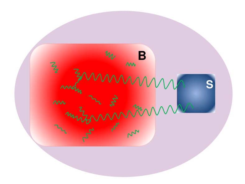
(a) Global interactions

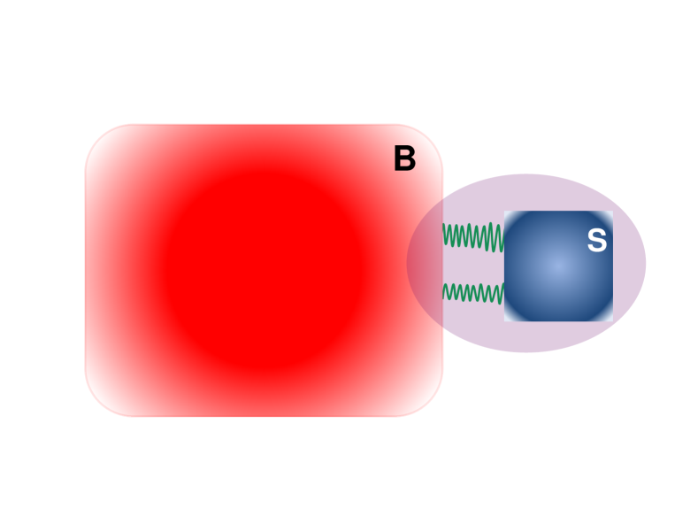
(b) Simple interactions

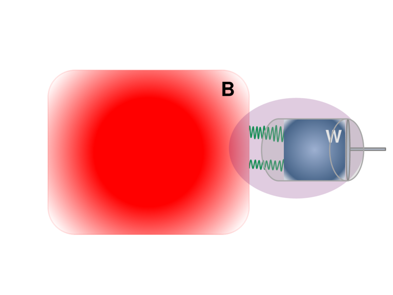
(b’) Classical thermodynamics - piston

Figure 1: Thermal operations vs. crude operations vs. classical operations. We consider a heat bath $B$ together with a system $S$ or working body $W$ and illustrate the different levels of control an experimenter can have on the setup and interactions. Figure (a): The most detailed, experimentally unfeasible control where the experimenter keeps a record of every microstate of the system and bath (the area contained within the purple oval) and controls interactions between the system and the entirety of the heat bath (illustrated by green stings). Figure (b): The desired level of control where the experimenter keeps track of the system and a small portion of the bath (purple oval) and performs some simple interactions between these regions (green strings). Figure (b’): The previous case can be regarded as analogous to the set up in traditional thermodynamics where one has a working body $W$ of which some parameters can be changed using simple processes such as moving a piston and weak couplings to the heat bath.

II Thermal Operations and Thermo-majorization

The thermo-majorization constraints were derived Horodecki and Oppenheim (2013) under the largest class of operations one is allowed to implement under thermodynamics - Thermal Operations Janzing et al. (2000); Streater (1995); Horodecki and Oppenheim (2013). These are presented in full detail in Section A.1 of the Appendix  but in particular they allow an experimenter to perform any energy conserving unitary between system and bath. Energy conservation does not pose a constraint on what is allowed since it can be enforced by incorporating a work storage device into the system to account for any energy excess of deficit. Rather, imposing energy conservation allows us to account for all sources of energy as is necessary for thermodynamics in the micro-regime. Clearly needing to apply all such unitaries to realize all possible transformations would require an enormous amount of control.

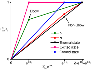
For a system in state $\rho$ and associated Hamiltonian $H_{S}$ with energy eigenstates $|i\rangle$, thermo-majorization assigns to each state a curve determined by the state’s energy levels $E_{i}$ and occupation probabilities $p_{i}=\mathop{\mathsf{tr}}\nolimits\left[\rho|i\rangle\langle i|\right]$. The construction of these curves is detailed and illustrated in Figure 2 (see also Section A.2 of the Appendix).

Figure 2: Thermo-majorization curves. The thermo-majorization curve for $\rho$ is defined by plotting the points: $\left\{\sum_{i=1}^{k}e^{-\beta E_{i}^{\left(\rho\right)}},\sum_{i=1}^{k}p_{i}^{\left(\rho\right)}\right\}_{k=1}^{n}$. The superscript $\left(\rho\right)$ indicates that the occupation probabilities and their associated energy levels have been ordered such that $p_{i}^{\left(\rho\right)}e^{\beta E_{i}^{\left(\rho\right)}}$ is non-increasing in $i$. This is called $\beta$-ordering. Note that states associated with the same Hamiltonian may have different $\beta$-orderings, as illustrated by $\rho$ and $\sigma$ here. We say that $\rho$ thermo-majorizes $\sigma$ as the thermo-majorization curve of $\rho$ is never below the thermo-majorization curve of $\sigma$. The thermo-majorization curve of a Gibbs state is given by a straight line between $\left(0,0\right)$ and $\left(Z,1\right)$. All other states thermo-majorize it. The pure state corresponding to the highest energy level of an $n$-level system thermo-majorizes all other states associated with that Hamiltonian. We call a point on a curve an elbow, if the gradient of the curve changes as it passes through the point. Otherwise, it is a non-elbow.

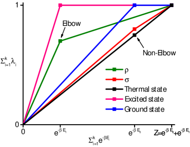
A system in state $\rho$ can be transformed into state $\sigma$ using at heat bath at inverse temperature $\beta=\frac{1}{kT}$ (here $k$ is Boltzmann’s constant) under thermal operations only if the thermo-majorization curve of $\rho$ is above that of $\sigma$. If $\sigma$ is block-diagonal in the energy eigenbasis or we have access to a source of coherence Brandão et al. (2013); Åberg (2014); Lostaglio et al. (2015); Ćwikliński et al. (2015), then they are sufficient too. In the thermodynamic limit, the thermo-majorization criteria collapses to the familiar second law: a transformation from $\rho$ to $\sigma$ is possible if and only if

$$F\left(\rho,H_{1}\right)\geq F\left(\sigma,H_{2}\right)$$

where $F\left(\rho,H\right)=\mathop{\mathsf{tr}}\nolimits\left[H\rho\right]-kTS\left(\rho\right)$ with $S\left(\rho\right)=-\mathop{\mathsf{tr}}\nolimits\left[\rho\log\rho\right]$ is the free energy. For the thermal state of the system $\tau_{\beta}$, $F\left(\tau_{\beta},H\right)=-kT\log Z$ where $Z=\sum_{i=1}^{d}e^{-\beta E_{i}}$ is the partition function. When the initial and final states are thermal states of their respective Hamiltonians, the difference in free energy equates to the optimal amount of work required (or gained) when transforming between the two states. For more general, nanoscopic states, thermo-majorization curves can be used to calculate the work required for a state transformation and we discuss this in Appendix A.3.

III Crude Operations

The first of our three basic operations are Partial Level Thermalizations (PLT). A thermalization essentially changes the state of the system into a thermal state and is usually achieved by putting the system in thermal contact with the reservoir until it equilibrates or by swapping the system with one from the reservoir. Thermalizations have no work cost or gain associated with it. A partial thermalization generalizes this, allowing one to thermalize with some probability $p$, implementing

$$\rho\rightarrow p\rho+\left(1-p\right)\tau_{\beta},$$

with $\tau_{\beta}$ being the thermal state at inverse temperature $\beta$. The probability $p$ can be determined by using the ambient heat bath as a source of noise or by putting the system in contact with it for a time shorter than the equilibration time.

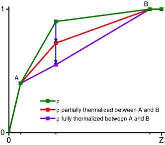
With Partial Level Thermalizations we go one step further and allow for the partial thermalization to act on any pair of energy levels. In order to implement them, one needs to be able to either perform the SWAP gate between any two levels of the system and of the thermal bath or to selectively put system energy levels in contact with the reservoir, for example by making use of an optical cavity or intermediate system which acts as a filter to restrict what energy levels are being addressed by the thermal contact. The action of PLTs on a state is illustrated in terms of thermo-majorization curves in Figure 3.

Figure 3: Action of Partial Level Thermalization. Here we illustrate the action of PLTs applied to a state $\rho$ over the two energy levels between points $A$ and $B$ for various degrees of thermalization $p$. Note, that as we apply the PLTs to adjacent energy levels with respect to the $\beta$-ordering of $\rho$, the final states maintain this $\beta$-order.

Our second type of operation are Level Transformations (LT), namely the raising and lowering of any subset of energy levels of the system’s Hamiltonian. This type of transformation is common within thermodynamics and the work cost of implementing them is given by the change in energy of the level (when the level is populated). Their effect on thermo-majorization is shown in Figure 4.

Figure 4: Action of Level Transformations. Here we illustrate the action of LTs applied to a system with a thermodynamical configuration $\left(\rho,H\right)$. Note that LTs leave the occupation probabilities of $\rho$ unchanged but may alter the $\beta$ ordering as discussed in the Appendix.

Finally, in the case where the system has degenerate energy levels, one may need to implement an energy conserving unitary acting within the degenerate subspace of the system. We will call this operation a Subspace Rotation (SR). It is only ever needed if the initial and final energy eigenstates are rotated with respect to each other and, in most examples we consider, it will not be needed and it does not effect the thermo-majorization curve of a state.

These operations are detailed with greater specificity in Section B of the Appendix, where it is also shown that they are a subset of Thermal Operations. Here, we shall contrast them with operations that have appeared in other resource theoretic approaches to thermodynamics. In Åberg (2013) it was shown that full thermalizations and Level Transformations suffice for extracting the optimal amount of work from a given state under Thermal Operations as evaluated in Horodecki and Oppenheim (2013). Similarly they can be used to form a given state from the thermal state at the same work cost as under TO.

In Egloff et al. (2015) it was shown, that for transitions between two diagonal states, perhaps with the expenditure or gain of work, it is enough to make thermal operations on the bath and the system, and instead of the work system used in Horodecki and Oppenheim (2013) just use level transformations. Still however, the system-bath coupling term used in Egloff et al. (2015) requires being able to implement an arbitrary Thermal Operations (see Renes (2014) and Renes (2015), where it is shown that the operations used in Egloff et al. (2015) are the subset of Thermal Operations) and thus requires in principle unlimited control.

Finally, in Skrzypczyk et al. (2014), a subset of Thermal Operations were considered which involved interacting with a designer heat bath which contained an arbitrarily large number of systems in a series of states that interpolated between the input state and the target state. Again, this would require an unfeasible amount of control in preparing the states of the heat bath.

As we shall see in the next Section, Crude Operations allow all transformations allowed by Thermal Operations to be implemented without the need for unreasonable levels of control.

IV Transformations using Crude Operations

In this paper, our goal is to consider the thermo-majorization curves of any two states in which the curve of $\rho$ lies above that of $\sigma$, and show that Level Transformations  Partial Level Thermalizations  and in some cases a Subspace Rotation, together with access to a single thermal qubit, are all that is needed to transform one curve into another.

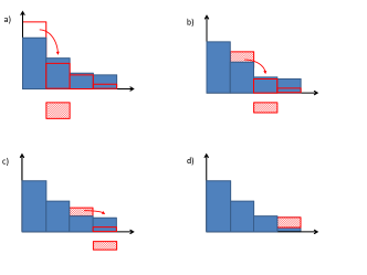
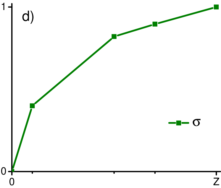
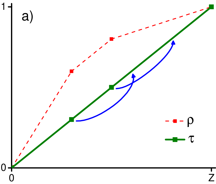
For the case where the Hamiltonian of the system is trivial, $H=0$, the thermo-majorization criteria is equivalent to the majorization criteria and any state $\rho$ can be transformed into any state $\sigma$ if and only if its eigenvalues majorize the eigenvalues of $\sigma$ Horodecki et al. (2003). That is, for respective sets of eigenvalues $\left\{p_{1},\dots,p_{d}\right\}$ and $\left\{q_{1},\dots,q_{d}\right\}$ written in non-decreasing order, $\rho\rightarrow\sigma$ is possible if and only if $\sum_{i=1}^{k}p_{i}\geq\sum_{i=1}^{k}q_{i}$, $\forall k$. In such a case, Muirhead Muirhead (1902) and Hardy, Littlewood, and Polya Hardy et al. (1952) showed that for states of dimension $d$ one can perform the transformation, using at most $d-1$ T-transforms. For $H=0$, where the thermal state is a maximally mixes state, these are just Partial Level Thermalizations. This is depicted in Figure 5 and discussed in the context of thermodynamics in Gour et al. (2015).

Figure 5: The heights of each column above are given by the probability of being in a particular eigenstate. The action of T-transforms transforms an initial state represented by red columns into the state represented by blue columns. The probabilities (column heights) of the red state majorizes those of the blue state. We work our way from left to right, moving probability mass from the red histogram to the right until it matches the blue histogram. In each step we move some probability mass from a column of the histogram of the initial state and move it to the right until it either matches the probability required of the target state, or until the left column of the initial state matches the right column of the final state. Red dashed rectangles represent the part of the column that is added to the next one due to the action of the T-transform.

However, in general such a protocol for $H=0$ does not extract any work during the state transformation. We show in Section F of the Appendix that by alternating Level Transformations and Partial Level Thermalizations one can make the transformation $\rho\rightarrow\sigma$ while extracting the optimal amount of work. We also show there how this can be accomplished in a physical set up involving a molecule in a box (a so called Szilard engine).

For an arbitrary Hamiltonian, the situation turns out to be much more complicated, as we will soon see. In fact, we will find that for an arbitrary state transformations, it is not enough to perform COs on the system alone, but that we need to perform COs on the system and an extra qubit in the thermal state.

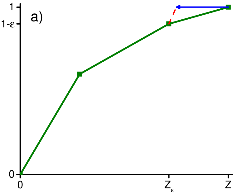
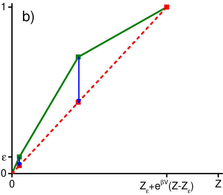
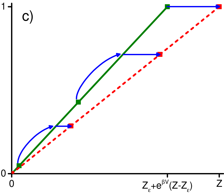
In the case where we want to extract the maximum amount of work from some state $\rho$ (i.e. transform $\rho$ into $\tau_{\beta}$), this can be achieved using Level Transformations and alternating Partial Level Thermalizations and Level Transformations. We term this alternating sequence a Partial Isothermal Reversible Process (PITR) in reference to the isothermal reversible processes defined in Åberg (2013) where Level Transformations are interlaced with full thermalizations to distil work. We discuss this work extraction protocol in Section E.1 of the Appendix and analyze the trade-off between the work extracted in the case where the protocol succeeds and the cost if it fails.

The reverse process to work extraction is that of formation. There one starts with the thermal state $\tau_{\beta}$ and uses work to form the state $\rho$. For the case where $\rho$ does not contain coherences, we construct a process to do this using Crude Operations in Section E.2 of the Appendix. The work cost of this protocol is optimal, requiring the same amount of work to be expended as under Thermal Operations.

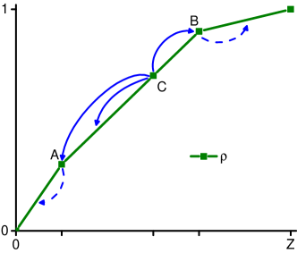
Both work extraction and formation make use of PITRs and these, and their associated work cost, are discussed more fully in Section B.3 of the Appendix. There we show that they provide a method to move non-elbows (as defined in Figure 2) to different segments of a thermo-majorization curve, without altering the curves shape and without expending any work. This is illustrated in Figure 6. Such a transformation will prove vital when we come to consider more general transformations.

Figure 6: Action of Partial Isothermal Reversible Processes. Here we illustrate the action of alternating Level Transformations and Partial Level Thermalizations (so-called, PITRs) applied to a system with state-Hamiltonian pair $\left(\rho,H\right)$. Using PITRs, the point at $C$ can be moved such that it lies anywhere on the line-segment between $A$ and $B$ and without changing the shape of the overall thermo-majorization curve. By performing this process sufficiently slowly, this can be done with no deterministic work cost. If one moves the point $C$ to coincide with point $A$ (respectively $B$), one can then use a second PITR to move point $A$ ($B$) as illustrated by the dashed arrows. Again, this does not alter the shape of the thermo-majorization curve.

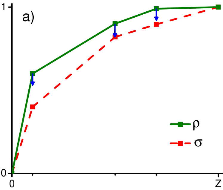
Transformations involving trivial Hamiltonian, and of distillation and formation in general, are straightforward because the initial and final states can be taken to be such that the elbows on their thermo-majorization curves are, respectively, vertically or horizontally aligned. For trivial Hamiltonians, all states have the same $\beta$-ordering and as such the points on the thermo-majorization diagrams for the initial and final states are vertically aligned. Building upon the results of Muirhead (1902) and Hardy et al. (1952), transformations between states with the same $\beta$-order can be performed by moving points vertically downwards using Partial Level Thermalizations. The protocol for achieving this is illustrated in Figure 7 and discussed in Section C of the Appendix. For work extraction and formation processes, the protocol is also simpler, since one of states is thermal and hence PITRs can be used to horizontally align its points with those of the other state for free. Transformations then just involve shifting points horizontally through Level Transformations.

(a) First PLT

(b) Second PLT

(c) Final PLT

(d) Final state, $\sigma$

Figure 7: Crude Operations protocol for transforming between states with the same $\beta$-order. If two states, $\rho$ and $\sigma$, have the same $\beta$-order and are such that $\rho$ thermo-majorizes $\sigma$, then $\rho$ can be converted into $\sigma$ using Partial Level Thermalizations. First a PLT is applied to $\rho$ across the complete set of energy levels, Figure (a), lowering the thermo-majorization of $\rho$ until it meets that of $\sigma$, Figure (b). Next, a second PLT is applied to those energy levels to the left of this meeting point, again lowering the curve until it meets that of $\sigma$ at a second point, Figure (c). By iterating this process, $\rho$ is transformed into $\sigma$, Figure (d).

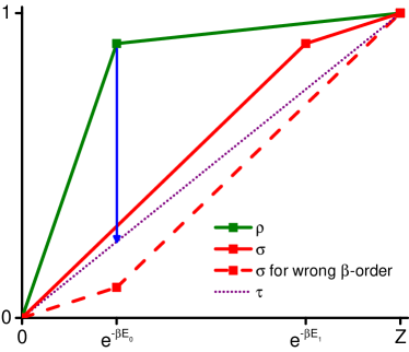
On the other hand, if the $\beta$-ordering between the initial and final state is different, then no method is known to transform $\rho$ into $\sigma$ using only Crude Operations acting on the system alone. The essential reason for this can be seen by looking at a qubit transformation where the initial and final state have different $\beta$-ordering as depicted in Figure 8. Essentially, we cannot write $\sigma=p\rho+(1-p)\tau_{\beta}$, and therefore, a Partial Level Thermalization cannot make $\rho\rightarrow\sigma$, nor can using any combination of LTs and PLTs.

Figure 8: Partial Level Thermalizations are not enough. Note that PLTs alone cannot implement all transitions possible under thermal operations. More specifically, they cannot implement changes of $\beta$-order on qubits. In the above example, we see that a PLT cannot take the initial state $\rho$ depicted in green to $\sigma$ depicted in red, because it first passes through the thermal state before it reaches $\sigma$ (which we have depicted in both its $\beta$-ordered, and non-$\beta$-ordered from). Because of this, work is required to go from $\rho$ to $\sigma$ even though the optimal process does not require work.

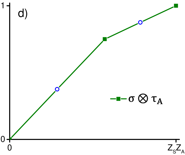
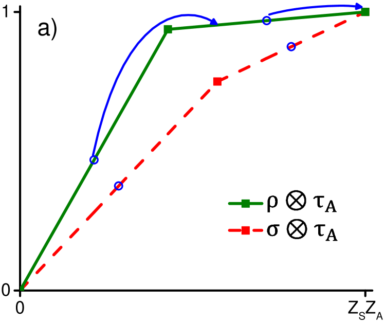
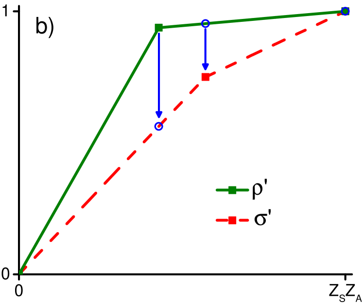
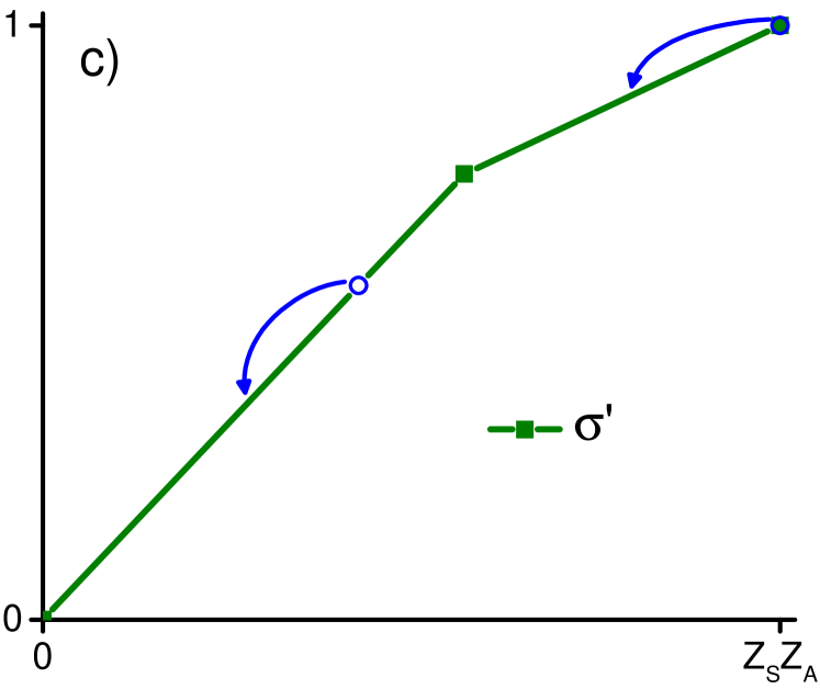
However, if we are able to perform Crude Operations, not just on the system, but on the system and a single qubit, $\tau_{A}$, from the thermal bath, then we show that one can transform $\rho$ into $\sigma$ even if the $\beta$-ordering is different. The protocol is given and explained in Section D and depicted in Figure 9. The idea is to convert this scenario back into one where the states under consideration have the same $\beta$-order. Appending $\tau_{A}$ adds additional non-elbow points to the thermo-majorization curve associated with $\rho$ and, by using PITRs, these can be moved so that they are vertically aligned with the elbows of the curve of $\sigma\otimes\tau_{A}$. Applying the protocol given in Figure 7 and a final round of PITRs to properly align the resulting non-elbow points, produces $\sigma\otimes\tau_{A}$. To the best of our knowledge, such a thermodynamical state transformation has never been performed in the lab.

(a) PITRs and PFs

(b) Same $\beta$-order protocol applied

(c) PITRs and PFs

(d) $\sigma\otimes\tau_{A}$

Figure 9: Crude Operations protocol for transforming between states with different $\beta$-orders. If $\rho$ thermo-majorizes $\sigma$, then it is possible to transform $\rho$ into $\sigma$ using Crude Operations. First, a thermal qubit, $\tau_{A}$, with known Hamiltonian is appended, Figure (a). Using Partial Isothermal Reversible Processes  the blue circles on the thermo-majorization curve of $\rho\otimes\tau_{A}$ can be moved to be vertically aligned with the ‘elbows’ on the curve for $\sigma\otimes\tau_{A}$. This forms the state $\rho^{\prime}$, Figure (b), that has a thermo-majorization curve overlapping that of $\rho\otimes\tau_{A}$. Using the previously defined protocol for states with the same $\beta$-order, $\rho^{\prime}$ can be converted into $\sigma^{\prime}$, Figure (c), that has a thermo-majorization curve overlapping that of $\sigma\otimes\tau_{A}$. A final round of PITRs converts $\sigma^{\prime}$ into $\sigma\otimes\tau_{A}$, Figure (d), and upon discarding $\tau_{A}$ we obtain $\sigma$.

V Conclusion

We have shown that Thermal Operations can be simulated by Crude Operations, a class of physical operations which can be implemented in the laboratory using current technology. This ought to bring thermodynamics of microscopic systems further into the experimental domain, and make the exploration of some of the results in the field Geusic et al. (1967); Alicki (1979); Gelbwaser-Klimovsky et al. (2013); Howard (1997); Geva and Kosloff (1992); Hänggi and Marchesoni (2009); Allahverdyan and Nieuwenhuizen (2000); Horodecki et al. (2003); Feldmann and Kosloff (2006); Linden et al. (2010); Dahlsten et al. (2011); Del Rio et al. (2011); Horodecki and Oppenheim (2013); Åberg (2013); Faist et al. (2012); Skrzypczyk et al. (2014); Brandao et al. (2015); Halpern and Renes (2014); Anders and Giovannetti (2013); Wilming et al. (2014); Mueller and Pastena (2015); Huber et al. (2015); Narasimhachar and Gour (2015); Alhambra et al. (2015); Woods et al. (2015) more feasible. From a conceptual point of view, this shows that the paradigm of thermodynamics which allows for the maximum amount of control of the system and bath, is in some sense equivalent to one which allows only very crude control of the system and bath. The second laws of thermodynamics, since they are fundamental limitations on state transitions, need to be derived assuming the experimenter has as much control and technology as would be allowed by nature (i.e. Thermal Operations). Yet remarkably, the fundamental limitation of thermo-majorization and generalized free energies, which are derived assuming maximal control, can be achieved with very little control, namely by COs. Control over bath degrees of freedom, with the exception of one qubit, is not needed.

There are additional second laws, which place constraints not only on the diagonal elements of the density matrix if written in the energy eigenbasis, but also place restrictions on the coherences over energy levels Brandao et al. (2015); Lostaglio et al. (2015); Ćwikliński et al. (2015); Lostaglio et al. (2015). While we expect Crude Operations are also sufficient for the control of quantum coherences, we do not yet know what the necessary conditions are for coherence manipulation, so verifying this is an important open question.

Acknowledgments Part of this work was carried out during the program ”Mathematical Challenges in Quantum Information” (2013) at the Isaac Newton Institute for Mathematical Sciences in the University of Cambridge and we thank them for their hospitality. J.O. is supported by an EPSRC Established Career Fellowship, the Royal Society, and FQXi. M.H. and P.Ć. thank EU grant RAQUEL. M.H. is also supported by Foundation for Polish Science TEAM project co-financed by the EU European Regional Development Fund. P.Ć. also acknowledges the support from the grant PRELUDIUM 2015/17/N/ST2/04047 from National Science Centre.

In this Appendix, we provide detailed protocols for simulating Thermal Operations with Crude Operations. We begin in Section A with a review of Thermal Operations, and the criteria for state transformations – thermo-majorization. Next, in B we introduce Crude Operations, describe each of the basic operations and show that they are a subset of Thermal Operations. We then consider the simpler case of transformations between states with the same $\beta$-ordering in Section C, showing that they can be performed using Crude Operations. In Section D we consider transitions between states where the $\beta$-ordering is different, and show that they can be achieved using Crude Operations. Quantifying the amount of work used in these processes is done in E. Finally, Section F, contains some very simple examples of state transitions in the case $H=0$, described using Szilard boxes. It serves an illustrative purpose, but also describes simple examples for extracting work while making a state transition. These were previously presented at Oppenheim (2013).

Appendix A Preliminaries

In this appendix, we recall and define relevant concepts and results from the resource theory of thermal operations (TO).

A.1 Thermal Operations

The resource theory of thermal operations Streater (1995); Janzing et al. (2000); Horodecki and Oppenheim (2013) is a way of more rigorously defining thermodynamics, and allows us to account for all sources of work and heat, something which needs to be done precisely when investigating the thermodynamics of a small system in the presence of a large heat bath. It is equivalent to other well studied paradigms of thermodynamics as shown in Brandão et al. (2013). Given a system in state $\rho$ with Hamiltonian $H$ and such a heat bath at temperature $T$, the following operations can be applied:

1. Since heat baths are a free resource, an ancillary system with any Hamiltonian, in the Gibbs state of that Hamiltonian at temperature $T$, can be appended as an ancilla. For the Hamiltonian $H_{B}=\sum_{i=1}^{n}E_{i}|i\rangle\langle i|$, the corresponding Gibbs state at temperature $T$ is defined as:

   $$\tau_{B}=\frac{1}{Z_{B}}\sum_{i=1}^{n}e^{-\beta E_{i}}|i\rangle\langle i|,$$ (1)

   where $\beta$ is the inverse temperature and $Z_{B}=\sum_{i=1}^{n}e^{-\beta E_{i}}$ is the partition function.

2. Any energy-conserving unitary, i.e. those unitaries that commute with the total Hamiltonian, can be applied to the global system. This is not a restriction, since any non-energy conserving unitary can be implemented using a work system and performing an energy conserving unitary on the work system and the original one. It does however allow us to properly account for work.

3. Any subsystem can be discarded through tracing out.

Given these, the action of a thermal operation on the state $\rho$ of a state-Hamiltonian pair $\left(\rho,H_{S}\right)$ at temperature $T$ can be written:

$$\rho\stackrel{{\scriptstyle\textrm{TO}}}{{\longrightarrow}}\mathop{\mathsf{tr}}\nolimits_{A}\left[U\left(\rho\otimes\tau_{B}\right)U^{\dagger}\right],$$ (2)

where $\tau_{B}$ is the Gibbs state of a Hamiltonian $H_{B}$, $A$ is the subsystem to be discarded and $U$ is a unitary such that:

$$\left[U,H_{S}+H_{B}\right]=0,$$ (3)

and we have used the shorthand notation $H_{S}+H_{B}=H_{S}\otimes\mathbb{I}_{B}+\mathbb{I}_{S}\otimes H_{B}$.

A.2 Thermo-majorization

Suppose we have a system $\left(\rho,H_{S}\right)$. Determining whether it can be transformed into the system $\left(\sigma,H_{S}\right)$ using thermal operations, can be formulated using thermo-majorization diagrams Horodecki and Oppenheim (2013).

Definition 1 (Thermo-majorization diagrams).

Given an $n$-level system, let $H_{S}=\sum_{i=1}^{n}E_{i}|i\rangle\langle i|$ be the system’s Hamiltonian and let us consider the energy occupation probabilities $\eta_{i}=\mathop{\mathsf{tr}}\nolimits{\rho|i\rangle\langle i|}$ To define the thermo-majorization curve of $\rho$, we first $\beta$-order the probabilities $\eta_{i}$ and energy levels, listing them such that $\eta_{i}e^{\beta E_{i}}$ is in non-increasing order.

The thermo-majorization curve of $\rho$ is then formed by plotting the $\beta$-ordered points:

$$\left\{\sum_{i=1}^{k}e^{-\beta E^{\left(\rho\right)}_{i}},\sum_{i=1}^{k}\eta_{i}^{\left(\rho\right)}\right\}_{k=1}^{n},$$ (4)

together with $\left(0,0\right)$, and connecting them piecewise linearly to form a concave curve. Here, the superscript $\left(\rho\right)$ on $E_{i}$ and $\eta_{i}$ indicate that they have been $\beta$-ordered and that this ordering depends on $\rho$.

An example of thermo-majorization diagrams is shown in Figure 10. We say that a state, thermo-majorizes another if its thermo-majorization curve never lies below that of the other.

Figure 10: Thermo-majorization curves. a) The thermo-majorization curve for $\rho$, is defined by plotting the points: $\left\{\sum_{i=1}^{k}e^{-\beta E_{i}^{\left(\rho\right)}},\sum_{i=1}^{k}\eta_{i}^{\left(\rho\right)}\right\}_{k=1}^{n}$. The superscript $\left(\rho\right)$ indicates that the occupation probabilities and their associated energy levels have been ordered such that $\eta_{i}^{\left(\rho\right)}e^{\beta E_{i}^{\left(\rho\right)}}$ is non-increasing in $i$. This is called $\beta$-ordering. Note that states associated with the same Hamiltonian may have different $\beta$-orderings, as illustrated by $\rho$ and $\sigma$ here. b) Here, we say that $\rho$ thermo-majorizes $\sigma$ as the thermo-majorization curve of $\rho$ is never below the thermo-majorization curve of $\sigma$. c) The thermo-majorization curve of a Gibbs state is given by a straight line between $\left(0,0\right)$ and $\left(Z,1\right)$. All other states thermo-majorize it. d) The pure state corresponding to the highest energy level of an $n$-level system thermo-majorizes all other states associated with that Hamiltonian. e) We call a point on a curve an elbow, if the gradient of the curve changes as it passes through the point. Otherwise, it is a non-elbow.

With these definitions in place, we can give the result of Horodecki and Oppenheim (2013):

Theorem 2 (Thermo-majorization).

Given two states $\rho$ and $\sigma$ of an $n$-level system with Hamiltonian $H_{S}$:

1. If $\sigma$ is block-diagonal in the energy eigenbasis, then $\rho\stackrel{{\scriptstyle\textrm{TO}}}{{\longrightarrow}}\sigma$, if and only if $\rho$ thermo-majorizes $\sigma$.

2. In general, $\rho\stackrel{{\scriptstyle\textrm{TO}}}{{\longrightarrow}}\sigma$, only if $\rho$ thermo-majorizes $\sigma$.

Thus, for states which are block diagonal in the energy basis, we have necessary and sufficient conditions to determine possible transitions between $\rho$ and $\sigma$. For quantum states with off-diagonal elements - coherences, the full set of constrains is only known in the case of a single qubit Ćwikliński et al. (2015), although various necessary conditions are known Brandao et al. (2015); Lostaglio et al. (2015); Ćwikliński et al. (2015); Lostaglio et al. (2015). On the other hand, if the experimenter is allowed access to a reference frame, then thermo-majorization is a necessary and sufficient condition for all state transformations Brandão et al. (2013); Åberg (2014); Lostaglio et al. (2015).

A.3 Wits and switch qubits

A.3.1 Work

In general, if we want a transition from $\rho$ to $\sigma$ to be possible, work may have to be added. Alternatively, if a transition can be achieved with certainty, it can be possible to extract work. Within the thermal operations framework, the optimal amount of work that must be added or can be gained, the work of transition, can be quantified using a continuous system, or for example the energy gap $W$ of a 2-level system, a wit Horodecki and Oppenheim (2013), with zero energy state $|0\rangle$ and an additional state $|1\rangle$. The associated Hamiltonian is:

$$H_{W}=W|1\rangle\langle 1|.$$ (5)

The deterministic work of transition, denoted $W_{\rho\rightarrow\sigma}$, is then defined to be the greatest value of $W$ such that the following holds:

$$\left(\rho\otimes|0\rangle\langle 0|,H_{S}+H_{W}\right)\stackrel{{\scriptstyle\textrm{TO}}}{{\longrightarrow}}\left(\sigma\otimes|1\rangle\langle 1|,H_{S}+H_{W}\right).$$ (6)

If $W_{\rho\rightarrow\sigma}$ is negative, to convert $\rho$ into $\sigma$ work has been taken from the work storage system to enable the transition to take place. On the other hand, if $W_{\rho\rightarrow\sigma}$ is positive, in converting $\rho$ into $\sigma$ it has been possible to store some extracted work in the work system.

Defining work in such a way enables the quantification of the worst-case work of a process. When $W_{\rho\rightarrow\sigma}$ is negative, it can be interpreted as the smallest amount of work that must be supplied to guarantee the transition. If it is positive, it is the largest amount of work we are guaranteed to extract in the process. As the work system is both initially and finally in a pure state, no entropy is stored in it and its energy change must be completely due to work being exchanged with the system. One can also quantify average work and consider fluctuations of the work system, however this does not change the considerations given here.

A.3.2 Changes of Hamiltonian

Thermodynamics is not just concerned with a system with Hamiltonian $H$ and whether it is possible to transform $\rho$ into $\sigma$ whilst keeping the $H$ fixed. One also wants to be able to consider transitions where the Hamiltonian changes, i.e.:

$$\left(\rho,H_{1}\right)\longrightarrow\left(\sigma,H_{2}\right),$$ (7)

and to determine the work cost or yield of performing such a change. Following Horodecki and Oppenheim (2013), this scenario can be mapped to one with identical initial and final Hamiltonian using the switch qubit construction. Here, we instead consider the transition between $\left(\rho\otimes|0\rangle\langle 0|\right)$ and $\left(\sigma\otimes|1\rangle\langle 1|\right)$ with Hamiltonian:

$$H=H_{1}\otimes|0\rangle\langle 0|+H_{2}\otimes|1\rangle\langle 1|.$$ (8)

Note that the partition function associated with $H$ is $Z=Z_{1}+Z_{2}$, where $Z_{1}$ and $Z_{2}$ are the partition functions of $H_{1}$ and $H_{2}$ respectively.

To model the work of transition in such a process, we combine this with Eq. (6) to give:

$$\left(\rho\otimes|0\rangle\langle 0|\otimes|0\rangle\langle 0|,H+H_{W}\right)\stackrel{{\scriptstyle\textrm{TO}}}{{\longrightarrow}}\left(\sigma\otimes|1\rangle\langle 1|\otimes|1\rangle\langle 1|,H+H_{W}\right),$$ (9)

and maximize over $W$.

Appendix B Crude Operations as thermal operations

In this appendix, we show how Crude Operations (CO) which we will now introduce are a subset of thermal operations.

Under Crude Operations the following operations can be applied:

1. A single 2-level system with known Hamiltonian, in the Gibbs state of that Hamiltonian at temperature $T$, can be appended as an ancilla.

2. Partial Level Thermalization (PLT) over any subset of energy levels.

3. Level Transformations (LT), provided the work cost is accounted for.

4. The ancilla system may be discarded.

5. Subspace Rotations (SR). Any energy conserving unitary $U$ such that $\left[U,H_{S}\right]=0$ may be applied to the system alone.

Operation 1 can obviously be realized using Operation 1 of thermal operations as described in Appendix A.1 but as we restrict to one ancillary system, the converse does not hold. As we shall see, Operation 2 can be realized using thermal operations whilst in general, Operation 3 may cost work to perform. Operation 5 is only ever used in the case of a degenerate energy eigenbasis and when the eigenbasis of the initial state does not match the energy eigenbasis of the target state. Let us now consider these operations in detail.

B.1 Partial Level Thermalizations

Partial Level Thermalizations act on a subset of a system’s energy levels, partially thermalizing the state supported on those levels. More formally:

Definition 3 (Partial Level Thermalization).

Given an $n$-level system with Hamiltonian $H_{S}=\sum_{i=1}^{n}E_{i}|i\rangle\langle i|$, a Partial Level Thermalization is parametrized by $\lambda\in\left[0,1\right]$ and acts on some subset of the system’s energy levels. Denote this subset of energy levels by $\mathcal{P}$ and the Partial Level Thermalization by $\textrm{PLT}_{\mathcal{P}}\left(\lambda\right)$.

The action of $\textrm{{PLT}}_{\mathcal{P}}\left(\lambda\right)$ on $\rho=\sum_{i=1}^{n}\eta_{i}|i\rangle\langle i|$, is defined by:

$$\rho\stackrel{{\scriptstyle\textrm{{PLT}}_{\mathcal{P}}\left(\lambda\right)}}{{\longrightarrow}}\rho^{\prime},$$ (10)

where $\rho^{\prime}=\sum_{i=1}^{n}\eta^{\prime}_{i}|i\rangle\langle i|$ and the $\eta^{\prime}_{i}$ are such that for $i\in\mathcal{P}$:

$$\eta^{\prime}_{i}=\left(1-\lambda\right)\eta_{i}+\frac{\lambda e^{-\beta E_{i}}}{\sum_{i\in\mathcal{P}}e^{-\beta E_{i}}}\sum_{i\in\mathcal{P}}\eta_{i},$$ (11)

and $\eta^{\prime}_{i}=\eta_{i}$ otherwise. The action of a Partial Level Thermalization, is illustrated in terms of thermo-majorization curves in Figure 11.

Figure 11: Action of Partial Level Thermalization. Here we illustrate the action of PLTs applied to a state $\rho$ over the two energy levels between points $A$ and $B$ for various degrees of thermalization. Note, that as we apply the PLTs to adjacent energy levels with respect to the $\beta$-ordering of $\rho$, the final states maintain this $\beta$-order.

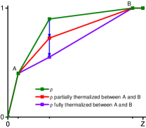
Note that such an operation preserves the $\beta$-ordering of the levels in $\mathcal{P}$ as, for $i,j\in\mathcal{P}$, if $\eta_{i}e^{\beta E_{i}}\geq\eta_{j}e^{\beta E_{j}}$, then $\eta^{\prime}_{i}e^{\beta E_{i}}\geq\eta^{\prime}_{j}e^{\beta E_{j}}$. In particular, if for some $d$, $\mathcal{P}=\left\{i^{\left(\rho\right)}\right\}_{i=k}^{k+d-1}$ (with the superscript $\left(\rho\right)$ denoting that the energy levels are $\beta$-ordered with respect to $\rho$), then $\rho^{\prime}$ will have the same $\beta$-ordering as $\rho$.

That Partial Level Thermalization form a subset of thermal operations, is captured in the following Lemma.

Lemma 4.

The map $\textrm{{PLT}}_{\mathcal{P}}\left(\lambda\right)$ can be implemented using thermal operations.

Proof.

To show this, we give an explicit protocol implementing a Partial Level Thermalization. For simplicity, we assume $\lambda$ is a positive rational of the form $\frac{a}{b}$ (if $\lambda$ is irrational, then $a$ and $b$ should be chosen such that the Partial Level Thermalization is implemented to the desired accuracy). Let the state of the system be $\rho=\sum_{i=1}^{n}\eta_{i}|i\rangle\langle i|$ and the associated Hamiltonian, $H_{S}=\sum_{i=1}^{n}E_{i}|i\rangle\langle i|$. The protocol then runs as follows:

• Step 1. Using Operation 1 of thermal operations:

  $$\left(\rho,H_{S}\right)\rightarrow\left(\rho\otimes\tau_{A}\otimes\mathbb{I}_{b},H_{S}+H_{A}+H_{M}\right),$$

  where $\tau_{A}$ is the Gibbs state of a $|\mathcal{P}|$-level system with Hamiltonian:

  $$H_{A}=\sum_{j\in\mathcal{P}}E_{j}|j\rangle\langle j|,$$

  and $\mathbb{I}_{b}$ is the maximally mixed state of dimension $b$. This is a Gibbs state of the $b$-level system with Hamiltonian $H_{M}=0$.

• Step 2. Let $\left\{|r_{S},s_{A},t_{M}\rangle\right\}$ be the set of orthonormal eigenvectors of $H_{S}+H_{A}+H_{M}$, each with associated energy level $E_{r}+E_{s}$. The eigenvalue of $\rho\otimes\tau_{A}\otimes\mathbb{I}_{b}$ associated with each energy level is $\frac{1}{bZ_{A}}\eta_{r}e^{-\beta E_{s}}$. Let $U$ be a unitary acting on the global system such that for $r\in\mathcal{P}$, $\forall s$, $t\in\left\{1,\dots,a\right\}$:

  $$U|r_{S},s_{A},t_{M}\rangle=|s_{S},r_{A},t_{M}\rangle,$$

  and $U|r_{S},s_{A},t_{M}\rangle=|r_{S},s_{A},t_{M}\rangle$ otherwise. By construction, $U$ is an energy conserving unitary that commutes with the total Hamiltonian.

• Step 3. Discard the two ancilla systems.

After applying this protocol, the population of energy level $E_{j}$ for $j\in\mathcal{P}$ is:

$$\eta_{j}-\frac{a}{bZ_{A}}\sum_{i\in\mathcal{P}}e^{-\beta E_{i}}\eta_{j}+\frac{a}{bZ_{A}}\sum_{i\in\mathcal{P}}e^{-\beta E_{j}}\eta_{i},$$

$$= \left(1-\frac{a}{b}\right)\eta_{j}+\frac{a}{b}\frac{e^{-\beta E_{j}}}{\sum_{i\in\mathcal{P}}e^{-\beta E_{i}}}\sum_{i\in\mathcal{P}}\eta_{i},$$

and $\eta_{j}$ otherwise. Comparing this with Eq. (11), we see that we have implemented the Partial Level Thermalization as required. ∎

B.2 Level Transformation

Level Transformations adjust the energy levels of a system’s Hamiltonian while keeping the state of the system fixed.

Definition 5 (Level Transformation).

Given an $n$-level system with Hamiltonian $H_{S}=\sum_{i=1}^{n}E_{i}|i\rangle\langle i|$ in the state $\rho=\sum_{i=1}^{n}\eta_{i}|i\rangle\langle i|$, a Level Transformation is parametrized by a set of real numbers $\mathcal{E}=\left\{h_{i}\right\}_{i=1}^{n}$ and denoted by $\textrm{LT}_{\mathcal{E}}$.

The action of $\textrm{LT}_{\mathcal{E}}$ on $\left(\rho,H_{S}\right)$ is:

$$\left(\rho,H_{S}\right)\stackrel{{\scriptstyle\textrm{LT}_{\mathcal{E}}}}{{\longrightarrow}}\left(\rho,H^{\prime}_{S}\right),$$ (12)

where:

$$H^{\prime}_{S}=\sum_{i=1}^{n}\left(E_{i}+h_{i}\right)|i\rangle\langle i|.$$ (13)

The single-shot, worst-case, work cost/yield of $\textrm{LT}_{\mathcal{E}}$ is defined by:

$$W_{\textrm{LT}_{\mathcal{E}}}=-\max_{i:\eta_{i}>0}h_{i}.$$ (14)

If $W_{\textrm{LT}_{\mathcal{E}}}$ is negative, work must be added for the transformation to happen deterministically while if it is positive, it may be possible to extract some work.

The action of a Level Transformation, is illustrated in terms of thermo-majorization curves in Figure 12.

Figure 12: Action of Level Transformations. Here we illustrate the action of LTs applied to a system with state-Hamiltonian pair $\left(\rho,H\right)$. Note that LTs leave the occupation probabilities of $\rho$ unchanged but may alter the $\beta$ ordering.

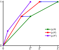
Level Transformation can be modeled within thermal operations using the wit and switch qubit discussed in Appendix A.3.

Lemma 6.

The map $\textrm{LT}_{\mathcal{E}}$ can be implemented using thermal operations with work cost at most $W_{\textrm{LT}_{\mathcal{E}}}$.

Proof.

Let $H=\sum_{i=1}^{n}E_{i}|i\rangle\langle i|$ be the initial Hamiltonian and $H^{\prime}=\sum_{i=1}^{n}E^{\prime}_{i}|i\rangle\langle i|$ be the final Hamiltonian after the application of $\textrm{LT}_{\mathcal{E}}$. Let $\mathcal{E}=\left\{h_{i}\right\}_{i=1}^{n}$ so $E^{\prime}_{i}=E_{i}+h_{i}$.

Consider modeling this transformation using the switch qubit construction:

$$H_{T}=H\otimes|0\rangle\langle 0|+H^{\prime}\otimes|1\rangle\langle 1|.$$

Let $H_{W}=W|1\rangle\langle 1|$ be the Hamiltonian for the wit. The work require to implement the Level Transformation  and convert the system $\left(\rho,H\right)$ into $\left(\rho,H^{\prime}\right)$ under thermal operations $W_{H\rightarrow H^{\prime}}$ is then given by the largest value of $W$ such that:

$$\left(\rho\otimes|0\rangle\langle 0|\otimes|0\rangle\langle 0|,H_{T}+H_{W}\right)\stackrel{{\scriptstyle\textrm{TO}}}{{\longrightarrow}}\left(\rho\otimes|1\rangle\langle 1|\otimes|1\rangle\langle 1|,H_{T}+H_{W}\right).$$

To see that $W_{H\rightarrow H^{\prime}}\geq W_{\textrm{LT}_{\mathcal{E}}}$, consider the Level Transformation parametrized by $\tilde{\mathcal{E}}=\left\{\tilde{h}_{i}\right\}_{i=1}^{n}$ where $\tilde{h}_{i}=W_{\textrm{LT}_{\mathcal{E}}}$, $\forall i$. Let $\tilde{H}$ denote the Hamiltonian obtained by applying $\textrm{LT}_{\tilde{\mathcal{E}}}$ to $H$ and note that the Level Transformation is such that $W_{\textrm{LT}_{\mathcal{E}}}=W_{\textrm{LT}_{\tilde{\mathcal{E}}}}$. To model this Level Transformation using thermal operations let:

$$\tilde{H}_{T}=H\otimes|0\rangle\langle 0|+\tilde{H}\otimes|1\rangle\langle 1|,$$

and its work cost under thermal operations $W_{H\rightarrow\tilde{H}}$ is given by the largest value of $W$ such that:

$$\left(\rho\otimes|0\rangle\langle 0|\otimes|0\rangle\langle 0|,\tilde{H}_{T}+H_{W}\right)\stackrel{{\scriptstyle\textrm{TO}}}{{\longrightarrow}}\left(\rho\otimes|1\rangle\langle 1|\otimes|1\rangle\langle 1|,\tilde{H}_{T}+H_{W}\right).$$

It can easily be seen that $W_{H\rightarrow\tilde{H}}=W_{\textrm{LT}_{\tilde{\mathcal{E}}}}$ and $W_{H\rightarrow\tilde{H}}\leq W_{H\rightarrow H^{\prime}}$. Hence the result follow. ∎

Note that this result implies that implementing the effect of a Level Transformation using a switch qubit and thermal operations, can be more cost-effective (in terms of work required to make the transformation deterministically) then performing a Level Transformation itself.

B.3 Partial Isothermal Reversible Processes and Points Flows

We can combine sequences of Level Transformations and (full) Partial Level Thermalizations (ie, with $\lambda=1$) in such a way to form a useful protocol, termed an Partial Isothermal Reversible Process as they are similar in construction to the Isothermal Reversible Processes considered in Åberg (2013) but require Partial Level Thermalizations rather than full thermalizations. Note, that a similar protocol to that of Partial Isothermal Reversible Processes was developed in Egloff et al. (2015) and termed an Isothermal shift of boundary. In terms of thermo-majorization curves, Partial Isothermal Reversible Processes will enable us to move non-elbow points along the segments on which they exist, without changing the shape and structure of the rest of the curve. More formally:

Definition 7 (Partial Isothermal Reversible Process).

Given an $n$-level system with Hamiltonian $H_{S}=\sum_{i=1}^{n}E_{i}|i\rangle\langle i|$, an Partial Isothermal Reversible Process is parametrized by a positive constant $\kappa$ and acts on some pair of the system’s energy levels, indexed by $j$ and $k$. Denote the Partial Isothermal Reversible Process by $\textrm{PITR}_{j,k}\left(\kappa\right)$.

The action of $\textrm{PITR}_{j,k}\left(\kappa\right)$ on $\left(\rho,H_{S}\right)$ where $\rho=\sum_{i=1}^{n}\eta_{i}|i\rangle\langle i|$, is defined by:

$$\left(\rho,H_{S}\right)\stackrel{{\scriptstyle\textrm{PITR}_{j,k}\left(\kappa\right)}}{{\longrightarrow}}\left(\rho^{\prime},H^{\prime}_{S}\right),$$ (15)

where $\rho^{\prime}=\sum_{i=1}^{n}\eta^{\prime}_{i}$ and $H^{\prime}_{S}=\sum_{i=1}^{n}E_{i}^{\prime}|i\rangle\langle i|$. Defining $\tilde{\eta}_{j}=\frac{e^{-\beta E_{j}}}{e^{-\beta E_{j}}+e^{-\beta E_{k}}}\left(\eta_{j}+\eta_{k}\right)$ and $\tilde{\eta}_{k}=\frac{e^{-\beta E_{k}}}{e^{-\beta E_{j}}+e^{-\beta E_{k}}}\left(\eta_{j}+\eta_{k}\right)$, the components of $\left(\rho^{\prime},H^{\prime}_{S}\right)$ in terms of $\kappa$ are then:

$$\begin{split}\eta^{\prime}_{j}&=\tilde{\eta}_{j}e^{-\beta\kappa},\\ \eta^{\prime}_{k}&=\tilde{\eta}_{k}+\left(1-e^{-\beta\kappa}\right)\tilde{\eta}_{j},\\ E^{\prime}_{j}&=E_{j}+\kappa,\\ E^{\prime}_{k}&=-\frac{1}{\beta}\ln\left[e^{-\beta E_{k}}+e^{-\beta E_{j}}\left(1-e^{-\beta\kappa}\right)\right],\end{split}$$ (16)

with $\eta^{\prime}_{i}=\eta_{i}$ and $E_{i}=E^{\prime}_{i}$ for $i\notin\left\{j,k\right\}$.

The action of an Partial Isothermal Reversible Process in terms of therm-majorization diagrams is illustrated in Figure 13.

Figure 13: Action of Partial Isothermal Reversible Processes. Here we illustrate the action of PITRs applied to a system with state-Hamiltonian pair $\left(\rho,H\right)$. Using PITRs, the point at $C$ can be moved such that it lies anywhere on the line-segment between $A$ and $B$ and without changing the shape of the overall thermo-majorization curve. By performing this process sufficiently slowly, this can be done with no deterministic work cost. If one moves the point $C$ to coincide with point $A$ (respectively $B$), one can then use a second PITR to move point $A$ ($B$) as illustrated by the dashed arrows. Again, this does not alter the shape of the thermo-majorization curve.

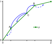
Note that in such a process, $Z_{S}=Z^{\prime}_{S}$ and that for all $\kappa$:

$$\eta^{\prime}_{j}e^{\beta E^{\prime}_{j}}=C=\eta^{\prime}_{k}e^{\beta E^{\prime}_{k}},$$ (17)

where $C$ is some constant.

The work cost of an Partial Isothermal Reversible Process is captured in the following Lemma which is similar in construction to that of (Egloff et al., 2015, Lemma 7.):

Lemma 8.

The operation $\textrm{PITR}_{j,k}\left(\kappa\right)$ does not cost any work.

Proof.

To show this, we define a $t$-step procedure that implements $\textrm{PITR}_{j,k}\left(\kappa\right)$ with each step consisting of a Level Transformation and a Partial Level Thermalization. Let $\left(\rho,H_{S}\right)$ and $\left(\rho^{\prime},H^{\prime}_{S}\right)$ be defined as per Definition 7. Without loss of generality, assume that:

$$\eta_{j}e^{\beta E_{j}}=C=\eta_{k}e^{\beta E_{k}}.$$

for some constant $C$ (if not, we can always perform $\textrm{{PLT}}_{\left\{j,k\right\}}\left(\lambda=1\right)$ to make it so and as by Lemma 4 this is a thermal operation, this costs no work). Hence in the language of Definition 7, $\eta_{j}=\tilde{\eta}_{j}$ and $\eta_{k}=\tilde{\eta}_{k}$.

Define $\epsilon=\frac{E^{\prime}_{j}-E_{j}}{t}$. Let the Hamiltonian after step $r$ be $H^{\left(r\right)}_{S}=\sum_{i=1}^{n}E^{\left(r\right)}_{i}|i\rangle\langle i|$ and the state of the system be $\rho^{\left(r\right)}=\sum_{i=1}^{n}\eta^{\left(r\right)}|i\rangle\langle i|$. In step $r$, we perform the level transformation such that:

$$E^{\left(r\right)}_{j} =E_{j}+r\epsilon,$$

$$E^{\left(r\right)}_{k} =-\frac{1}{\beta}\ln\left[e^{-\beta E_{k}}+e^{-\beta E_{j}}\left(1-e^{-\beta r\epsilon}\right)\right]$$

and fully thermalize over energy levels $j$ and $k$ so that:

$$\eta^{\left(r\right)}_{j} =\eta_{j}e^{-\beta r\epsilon},$$

$$\eta^{\left(r\right)}_{k} =\eta_{k}+\left(1-e^{-\beta r\epsilon}\right)\eta_{j}.$$

All other energy levels and occupation probabilities remain unchanged. It can readily be verified that $Z^{\left(r\right)}_{S}=Z_{S}$ and that:

$$\eta^{\left(r\right)}_{j}e^{\beta E^{\left(r\right)}_{j}}=C=\eta^{\left(r\right)}_{k}e^{\beta E^{\left(r\right)}_{k}}.$$

Hence, this protocol produces the desired $\left(\rho^{\prime},H_{S^{\prime}}\right)$ after $t$ steps.

Such a protocol alters the state and Hamiltonian of the system but does not change the shape of the system’s thermo-majorization curve. Following the proof of (Åberg, 2013, Supplementary Lemma 1.) regarding Isothermal Reversible Processes, we shall now show that the work cost of this protocol becomes increasingly peaked around zero as the number of steps taken tends to infinity.

Let $W^{\left(r\right)}$ denote the random variable for the work distribution in step $r$ of the PITR. The work distribution for the whole $t$-step PITR process is then:

$$W^{\textrm{PITR}}=\sum_{r=1}^{t}W^{\left(r\right)}.$$

Using Eqs. (16) and (17), $W^{\left(r\right)}$ is such that with probability:

$$Ce^{-\beta E_{j}^{\left(r\right)}}, \quad W^{\left(r\right)}=\epsilon,$$

$$Ce^{-\beta E_{k}^{\left(r\right)}}, \quad W^{\left(r\right)}=-\frac{1}{\beta}\ln\left[e^{-\beta E^{\left(r\right)}_{k}}+e^{-\beta E^{\left(r\right)}_{j}}\left(1-e^{-\beta\epsilon}\right)\right]-E^{\left(r\right)}_{k},$$

$$\textrm{otherwise}, \quad W^{\left(r\right)}=0.$$

Now, for large $t$, small $\epsilon$, this becomes such that with probability:

$$Ce^{-\beta E_{j}^{\left(r\right)}}, \quad W^{\left(r\right)}=\epsilon,$$

$$Ce^{-\beta E_{k}^{\left(r\right)}}, \quad W^{\left(r\right)}=-\epsilon e^{\beta\left(E^{\left(r\right)}_{k}-E^{\left(r\right)}_{j}\right)}+O(\epsilon^{2}),$$

$$\textrm{otherwise}, \quad W^{\left(r\right)}=0.$$

Hence as $t\rightarrow\infty$, $\left\langle W^{\left(r\right)}\right\rangle\rightarrow 0$, for all $r$. As $t=\frac{E^{(t)}_{j}-E^{(0)}_{j}}{\epsilon}=\frac{E^{\prime}_{j}-E_{j}}{\epsilon}$, we have that:

$$\left\langle W^{\textrm{PITR}}\right\rangle=\sum_{r=1}^{t}\left\langle W^{\left(r\right)}\right\rangle\rightarrow 0,\quad\textrm{as }t\rightarrow\infty.$$

Now consider the variance of $W^{\textrm{PITR}}$. For large $t$, hence small $\epsilon$:

$$\left\langle{W^{\left(r\right)}}^{2}\right\rangle =Ce^{-\beta E^{\left(r\right)}_{j}}\epsilon^{2}+Ce^{-\beta E^{\left(r\right)}_{k}}\epsilon^{2}e^{2\beta\left(E^{\left(r\right)}_{k}-E^{\left(r\right)}_{j}\right)}+O(\epsilon^{4})$$

$$=Ce^{-\beta E^{\left(r\right)}_{j}}\epsilon^{2}\left(1+e^{\beta\left(E^{\left(r\right)}_{k}-E^{\left(r\right)}_{j}\right)}\right)+O(\epsilon^{4})$$

$$\rightarrow 0\quad\textrm{as }\epsilon\rightarrow 0.$$

Hence, $\textrm{Var}\left(W^{\left(r\right)}\right)\rightarrow 0$ as $t\rightarrow\infty$. As the $W^{\left(r\right)}$ are independent:

$$\textrm{Var}\left(W^{\textrm{PITR}}\right) =\sum_{r=1}^{t}\textrm{Var}\left(W^{\left(r\right)}\right)$$

$$\rightarrow 0\quad\textrm{as }\epsilon\rightarrow 0.$$

Note that this analysis extends to the case where $E^{\prime}_{j}\rightarrow\infty$. If we parametrize $E^{\prime}_{j}$ in terms of the number of steps taken in the PITR protocol so that $E^{\prime}_{j}=\ln t$, then in the limit $t\rightarrow\infty$, $E^{\prime}_{j}\rightarrow\infty$, $\left\langle W^{\textrm{PITR}}\right\rangle\rightarrow 0$ and $\textrm{Var}\left(W^{\textrm{PITR}}\right)\rightarrow 0$.

Now, Chebyshev’s inequality gives us that:

$$P\left(\left|W^{\textrm{PITR}}\right|\geq k\sqrt{\textrm{Var}\left(W^{\textrm{PITR}}\right)}\right)\leq\frac{1}{k^{2}},$$

so by taking $t$ and $k$ to be large, we obtain that the work distribution for the PITR becomes increasingly peaked around 0. ∎

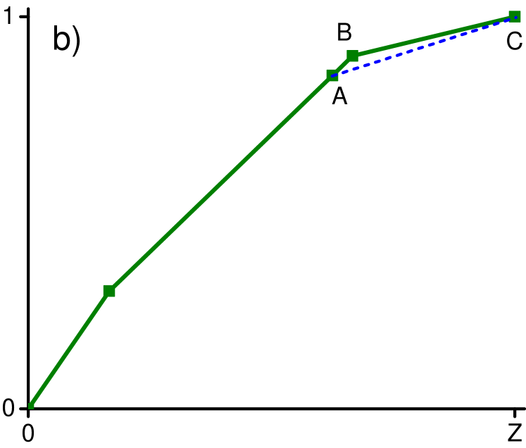
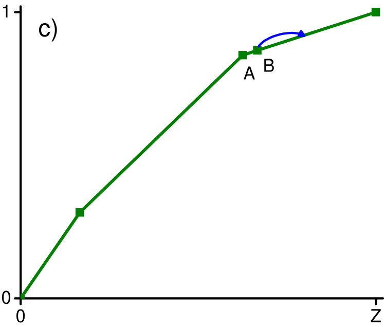
Hence, Partial Isothermal Reversible Processes can be used to move non-elbow points along straight-line segments of a thermo-majorization curve, using Crude Operations and without expending any work. By combining two PITRs, it is possible to commute non-elbow points with elbows, meaning that non-elbows can be moved to any point of the thermo-majorization curve for free. We term this operation Exact Points Flow.

Definition 9 (Exact Points Flow (EPF)).

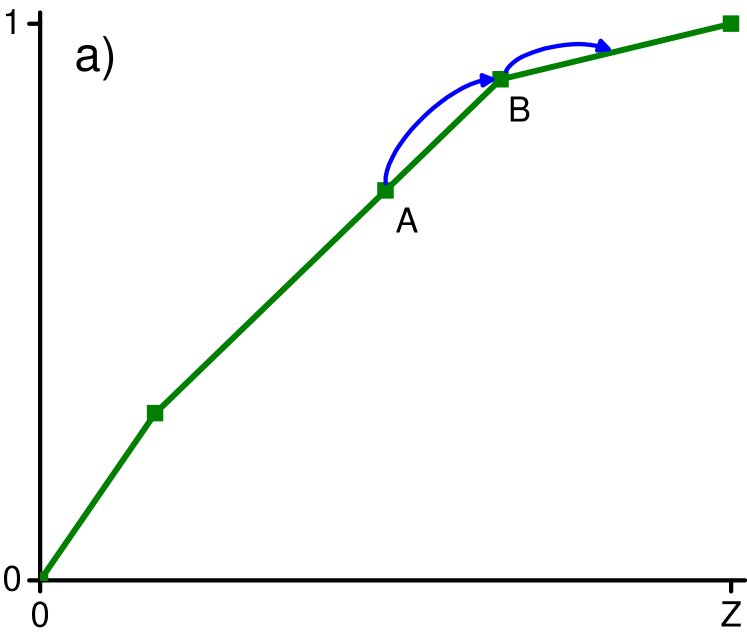
Exact Points Flow is illustrated in Figure 14. Given an $n$-level system with Hamiltonian $H_{S}=\sum_{i=1}^{n}E_{i}|i\rangle\langle i|$ and state $\rho=\sum_{i=1}^{n}\eta_{i}|i\rangle\langle i|$ such that:

$$\eta_{j}e^{\beta E_{j}}=\eta_{k}e^{\beta E_{k}},$$ (18)

for some $j,k$ (i.e. there is a non-elbow point on the thermo-majorization curve), an Exact Points Flow moves this non-elbow to another part of the thermo-majorization curve whilst keeping the shape of the curve fixed.

To implement EPF, we first apply a PITR that sends $E_{j}\rightarrow\infty$. This lowers the energy of $E_{k}$ and does not alter the shape of the thermo-majorization curve. Next, to move the non-elbow to another part of the curve, we apply another PITR to $j$ and a third level labeled by $l$, bringing the energy level associated with $j$ back down from infinity to some $E^{\prime}_{j}$. This leaves us with a system $\left(\rho^{\prime},H^{\prime}_{S}\right)$ with thermo-majorization curve identical to that of $\left(\rho,H_{S}\right)$ and such that:

$$\eta^{\prime}_{j}e^{\beta E^{\prime}_{j}}=\eta^{\prime}_{l}e^{\beta E^{\prime}_{l}},$$ (19)

(i.e. the elbow defined in Eq. (18) has moved to another part of the curve).

(a) Initial state.

(b) Final state.

Figure 14: Exact Points Flow. Here we illustrate how to move a non-elbow point through an elbow. First, we perform a PITR that sends the non-elbow, $A$, towards the elbow, $B$. As the appropriate energy level is raised to infinity during the protocol, $A$ tends towards $B$ until they coincide. Next, a second PITR lowers the energy level from infinity, keeping it in partial thermal equilibrium with respect to another line-segment. This moves $B$, now a non-elbow, to this new line-segment.

We also present an example of Exact Points Flow showing what happens with energy levels and how the points are moved with respect to Gibbs weights in Figure 15.

$\begin{array}[]{ccccc}\includegraphics[width=173.44534pt,height=157.33412pt]{supplementary_figures/flow_ex}&\qquad\includegraphics[width=173.44534pt,height=157.33412pt]{supplementary_figures/flow_example_1}\\ \includegraphics[width=173.44534pt,height=157.33412pt]{supplementary_figures/flow_example_2}\end{array}$

Figure 15: Points Flow - example with infinity

Exact Points Flow requires that an energy level is raised to infinity during a Partial Isothermal Reversible Process. If it is not possible, or undesirable, to raise an energy level to infinity, a similar effect to an Exact Points Flow can be achieved while altering the shape of the thermo-majorization curve slightly in a process we call Approximate Points Flow.

Definition 10 (Approximate Points Flow (APF)).

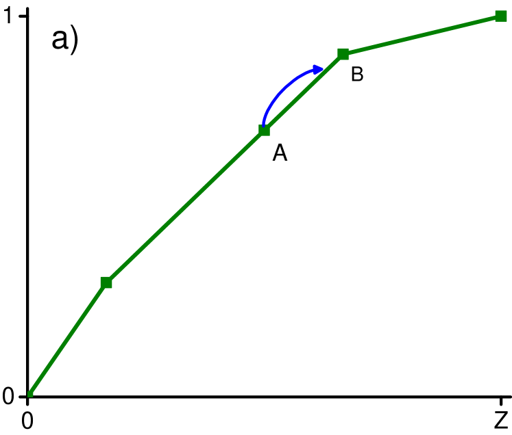
Approximate Points Flow is illustrated in Figure 16. Given an $n$-level system with Hamiltonian $H_{S}=\sum_{i=1}^{n}E_{i}|i\rangle\langle i|$ and state $\rho=\sum_{i=1}^{n}\eta_{i}|i\rangle\langle i|$ such that:

$$\eta_{j}e^{\beta E_{j}}=\eta_{k}e^{\beta E_{k}},$$ (20)

for some $j,k$ (i.e. there is a non-elbow point on the thermo-majorization curve), an Approximate Points Flow moves this non-elbow to an adjacent segment of the thermo-majorization curve whilst modifying the shape of the thermo-majorization curve by an arbitrarily small amount and without sending an energy level to infinity.

To implement it, without loss of generality, assume that the set $\left\{i\right\}_{i=1}^{n}$ has been $\beta$-ordered, we wish to move the non-elbow point to the right and take $j=k+1$. To do this, we:

1. Apply a PITR that raises the energy level of $E_{j}$ to some fixed, large but finite amount. This lowers the energy of $E_{k}$ and does not alter the shape of the thermo-majorization curve.

2. We now apply:

   $$\textrm{{PLT}}_{\left\{j,j+1\right\}}\left(\lambda=1\right),$$ (21)

   to the system. This turns the non-elbow associated with $j$ and $k$ into an elbow and the elbow associated with $j$ and $j+1$ into a non-elbow.

3. Using a PITR, we can now move the new non-elbow point without altering the shape of the thermo-majorization curve.

(i.e. the elbow defined in Eq. (18) has moved to another part of the curve). By adjusting the height to which $E_{j}$ is raised in Step 1, we can tune the extent to which the thermo-majorization curve is altered.

(a) Initial State

(b) After first PITR.

(c) After PLT.

(d) After second PITR.

Figure 16: Approximate Points Flow. Here we illustrate the protocol of Approximate Points Flow using thermo-majorization diagrams. Initially the system is as per Figure (a). Using a PITR, the non-elbow point, $A$, is moved towards the elbow at point $B$. This results in Figure (b). Next, a PLT is applied between points $A$ and $C$, leading to Figure (c). Point $B$ is now a non-elbow and can be moved using a PITR, giving Figure (d).

B.4 Subspace Rotation

Subspace Rotations are only needed in the case when the eigenbasis of the initial state or target state are not diagonal in the energy eigenbasis. Since the thermo-majorization criteria is about transitions between energy eigenstates, we want to consider transitions to and from energy eigenstates. Since we are only considering such transitions, we can, as described in Horodecki and Oppenheim (2013), take the target state to be block-diagonal in the energy eigenbasis $\sigma=\sum\eta_{i}^{(\sigma)}|i\rangle\langle i|$, which one can also show allows one to consider only initial states which are block-diagonal. However, the eigenbasis of the initial and final state, even if block diagonal in the energy eigenbasis, may not be the same. In such a case we use a Subspace Rotation to rotate the state, either initially, or at the end of the protocol. Note also that if an SR is applied at random, then it also serves to decohere in the energy eigenbasis of the system if that is desired. As the unitary is applied only to the system under consideration, it is much easier to implement experimentally than a more general thermal operation. We will henceforth assume that if needed, an SR has been applied to the initial state, or will be applied at the end of the protocol, such that we need only consider transitions between states which are both diagonal in the energy eigenbasis.

Appendix C Transformations for states with same $\beta$-order

In this appendix, we show that for two states with the same $\beta$-ordering, if one thermo-majorizes the other, then the transition can be made using a finite number of Partial Level Thermalizations. Furthermore, these Partial Level Thermalizations need only act on two energy levels at a time.

We say that two states $\rho$ and $\sigma$, associated with the same Hamiltonian $H_{S}=\sum_{i=1}^{n}E_{i}|i\rangle\langle i|$, have the same $\beta$-ordering if:

$$\sum_{i=1}^{k}e^{-\beta E^{\left(\rho\right)}_{i}}=\sum_{i=1}^{k}e^{-\beta E^{\left(\sigma\right)}_{i}},\quad\forall k.$$ (22)

Theorem 11.

Suppose that $\rho$ and $\sigma$ are states of an $n$-level system with Hamiltonian $H_{S}=\sum_{i=1}^{n}E_{i}|i\rangle\langle i|$ such that:

1. $\sigma$ is block-diagonal in the energy eigenbasis.

2. $\rho$ and $\sigma$ have the same $\beta$-order.

3. $\rho\stackrel{{\scriptstyle\textrm{TO}}}{{\longrightarrow}}\sigma$.

Then $\rho$ can be converted into $\sigma$ using at most $n-1$ Partial Level Thermalizations.

Proof.

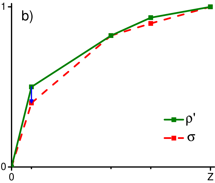
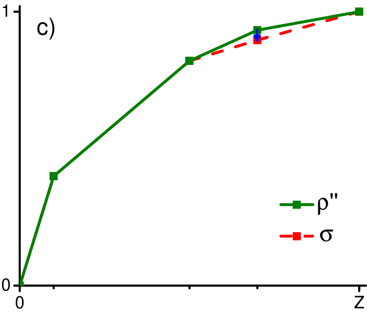
To prove this, we give a protocol consisting only of Partial Level Thermalizations that converts $\rho$ into $\sigma$. An illustrative outline for the protocol is given in Figure 17. As we can perform any energy conserving unitary on the system, we can assume that both $\rho$ and $\sigma$ are diagonal in the energy eigenbasis (by decohering $\rho$ if necessary).

Let $\left\{\eta_{i}\right\}_{i=1}^{n}$ be the $\beta$-ordered eigenvalues of $\rho$, $\left\{\zeta_{i}\right\}_{i=1}^{n}$ be the $\beta$-ordered eigenvalues of $\sigma$ and $\left\{E_{i}\right\}_{i=1}^{n}$ be the $\beta$-ordered energy-eigenvalues of $H_{S}$.

Given that $\rho$ and $\sigma$ have the same $\beta$-order, $\rho$ majorizes $\sigma$ if and only if:

$$\sum_{i=1}^{m}\eta_{i}\geq\sum_{i=1}^{m}\zeta_{i},\quad\forall m.$$ (23)

Let $\mathcal{M}$ be the set of $m$ for which equality occurs in Eq. (23). Suppose that are $r$ of them, and label them in ascending order by $\left\{t_{s}\right\}_{s=1}^{r}$. Note that $t_{r}=n$ and for convenience, define $t_{0}=0$.

We now proceed to perform a PLT on each set of energy levels $\mathcal{P}^{s}\equiv\left\{t_{s-1}+1,\dots,t_{s}-1\right\}$ for $1\leq s\leq r$. For each $m\in\mathcal{P}^{s}$, let $\lambda^{s}_{m}$ be defined as the solution to:

$$\sum_{j=t_{s-1}+1}^{m}\left[\left(1-\lambda^{s}_{m}\right)\eta_{j}+\frac{\lambda^{s}_{m}e^{-\beta E_{j}}}{\sum_{l\in\mathcal{P}^{s}}e^{-\beta E_{l}}}\sum_{l\in\mathcal{P}^{s}}\eta_{l}\right]=\sum_{j=t_{s-1}+1}^{m}\zeta_{j},$$ (24)

i.e. $\lambda^{s}_{m}$ is such that if one were to apply $\textrm{PT}_{\mathcal{P}^{s}}\left(\lambda^{s}_{m}\right)$ to $\rho$, the thermo-majorization curve of the resultant state would touch or cross the thermo-majorization curve of $\sigma$ at $m$. To ensure the resultant state thermo-majorizes $\sigma$, we actually apply the transformation $\textrm{PT}_{\mathcal{P}^{s}}\left(\lambda^{s}_{\textrm{min}}\right)$ for each $s$ where:

$$\lambda^{s}_{\textrm{min}}=\min_{m\in\left\{t_{s-1}+1,\dots,t_{s}-1\right\}}\lambda^{s}_{m}.$$ (25)

This leaves us with a state $\rho^{\prime}$ that has the same $\beta$-ordering as $\rho$ and $\sigma$ and thermo-majorizes $\sigma$.

Let $\left\{\eta^{\prime}_{i}\right\}_{i=1}^{n}$ be the $\beta$-ordered eigenvalues of $\rho^{\prime}$. Then $r^{\prime}$, the number of $m$ such that:

$$\sum_{i=1}^{m}\eta^{\prime}_{i}=\sum_{i=1}^{m}\zeta_{i},$$ (26)

is greater than or equal to $r$ with equality if and only if $r=n$. Hence by iterating the above procedure at most $n-1$ times, we transform $\rho$ into $\sigma$ using Partial Level Thermalizations. ∎

(a) First PLT

(b) Second PLT

(c) Final PLT

(d) Final state, $\sigma$

Figure 17: Crude Operations protocol for transforming between states with the same $\beta$-order. If two states, $\rho$ and $\sigma$, have the same $\beta$-order and are such that $\rho$ thermo-majorizes $\sigma$, then $\rho$ can be converted into $\sigma$ using Partial Level Thermalizations. First a PLT is applied to $\rho$ across the complete set of the energy levels, Figure (a), lowering the thermo-majorization of $\rho$ until it meets that of $\sigma$, Figure (b). Next, a second PLT is applied to those energy levels to the left of this meeting point, again lowering the curve until it meets that of $\sigma$ at a second point, Figure (c). By iterating this process, $\rho$ is transformed into $\sigma$, Figure (d).

Partial Level Thermalizations that act on 2 energy levels at a time are analogous to the concept of $T$-transforms (see, for example, (Marshall et al., 2010, Chapter 2, Section B)) in majorization theory. Within majorization theory, it is know that if the vector $\vec{v}$ majorizes $\vec{u}$, then $\vec{v}$ can be converted into $\vec{u}$ using a finite number of $T$-transforms Muirhead (1902); Hardy et al. (1952). The equivalent result for thermo-majorization is captured in the following theorem:

Theorem 12.

Suppose that $\rho$ and $\sigma$ are states of an $n$-level system with Hamiltonian $H_{S}=\sum_{i=1}^{n}E_{i}|i\rangle\langle i|$ such that:

1. $\sigma$ is block-diagonal in the energy eigenbasis.

2. $\rho$ and $\sigma$ have the same $\beta$-order.

3. $\rho\stackrel{{\scriptstyle\textrm{TO}}}{{\longrightarrow}}\sigma$.

Then $\rho$ can be converted into $\sigma$ using at most $n-1$ Partial Level Thermalizations that each act on 2 energy levels.

Proof.

The aim is to construct a protocol consisting of such PLTs that converts $\rho$ into $\sigma$. To do this, we perform a sequence of PLTs. Each PLT adjusts the gradients of two line-segments of the thermo-majorization curve of $\rho$ until one of them matches the gradient of the corresponding segment on $\sigma$. By picking the segments of $\rho$ such that one has gradient strictly greater than the corresponding segment on $\sigma$ and one has gradient strictly less than the corresponding segment on $\sigma$ this can always be done. Once all of the gradients have been matched, $\rho$ has been converted into $\sigma$. The full details of the protocol are below. Again, by first imagining that we have decohered $\rho$ in the energy eigenbasis if necessary, we can assume that $\rho$ and $\sigma$ are diagonal in the energy eigenbasis.

Let $\left\{\eta_{i}\right\}_{i=1}^{n}$ be the $\beta$-ordered eigenvalues of $\rho$, $\left\{\zeta_{i}\right\}_{i=1}^{n}$ be the $\beta$-ordered eigenvalues of $\sigma$ and $\left\{E_{i}\right\}_{i=1}^{n}$ be the $\beta$-ordered energy-eigenvalues of $H_{S}$. Hence we have:

$$\eta_{1}e^{\beta E_{1}}\geq\dots\geq\eta_{n}e^{\beta E_{n}},$$ (27)

and

$$\zeta_{1}e^{\beta E_{1}}\geq\dots\geq\zeta_{n}e^{\beta E_{n}}.$$ (28)

Given that $\rho$ and $\sigma$ have the same $\beta$-order, $\rho$ majorizes $\sigma$ if and only if:

$$\sum_{i=1}^{m}\eta_{i}\geq\sum_{i=1}^{m}\zeta_{i},\quad\forall m.$$ (29)

Let $j$ be the largest index such that $\eta_{j}e^{\beta E_{j}}>\zeta_{j}e^{\beta E_{j}}$ and $k$ be the smallest index larger than $j$ such that $\eta_{k}e^{\beta E_{k}}<\zeta_{k}e^{\beta E_{k}}$. This picks the segments we shall apply the PLT to. Then:

$$\eta_{j}e^{\beta E_{j}}>\zeta_{j}e^{\beta E_{j}}\geq\zeta_{k}e^{\beta E_{k}}>\eta_{k}e^{\beta E_{k}},$$ (30)

and note that $\eta_{i}=\zeta_{i}$ for $j<i<k$.

We now determine the amount that we need to thermalize by in order to transform the gradient of one of the segments of $\rho$ to that of $\sigma$. Define $\lambda_{1}$ to be the value of $\lambda$ such that:

$$\left(1-\lambda_{1}\right)\eta_{j}e^{\beta E_{j}}+\frac{\lambda_{1}\left(\eta_{j}+\eta_{k}\right)}{e^{-\beta E_{j}}+e^{-\beta E_{k}}}=\zeta_{j}e^{\beta E_{j}},$$ (31)

and $\lambda_{2}$ to be such that:

$$\left(1-\lambda_{2}\right)\eta_{k}e^{\beta E_{k}}+\frac{\lambda_{2}\left(\eta_{j}+\eta_{k}\right)}{e^{-\beta E_{j}}+e^{-\beta E_{k}}}=\zeta_{k}e^{\beta E_{k}}.$$ (32)

Note that:

$$\eta_{j}e^{\beta E_{j}}\geq\frac{\eta_{j}+\eta_{k}}{e^{-\beta E_{j}}+e^{-\beta E_{k}}}\geq\eta_{k}e^{\beta E_{k}},$$ (33)

and hence $\lambda_{1},\lambda_{2}\geq 0$. Also, at least one of $\frac{\left(\eta_{j}+\eta_{k}\right)}{e^{-\beta E_{j}}+e^{-\beta E_{k}}}\leq\zeta_{j}e^{\beta E_{j}}$ or $\frac{\left(\eta_{j}+\eta_{k}\right)}{e^{-\beta E_{j}}+e^{-\beta E_{k}}}\geq\zeta_{k}e^{\beta E_{k}}$ holds as $\zeta_{j}e^{\beta E_{j}}\geq\zeta_{k}e^{\beta E_{k}}$. Hence at least one of $\lambda_{1}$ and $\lambda_{2}$ must lie in the interval $\left[0,1\right]$. Let:

$$\lambda=\min\left\{\lambda_{1},\lambda_{2}\right\}.$$ (34)

Let $\rho^{\prime}$ be the state formed by applying the 2-level Partial Level Thermalization $\textrm{{PLT}}_{\left\{j,k\right\}}\left(\lambda\right)$ to $\rho$. Note that $\rho^{\prime}$ has the same $\beta$-order as $\rho$ and $\sigma$. To see this, let $\left\{\eta^{\prime}_{i}\right\}_{i=1}^{n}$ be the eigenvalues of $\rho^{\prime}$ listed according to the $\beta$ ordering of $\rho$. Then:

$$\eta^{\prime}_{i} =\eta_{i},\quad\textrm{for }1\leq i<j,$$

$$\eta^{\prime}_{i} =\zeta_{i},\quad\textrm{for }j<i<k,$$

$$\eta^{\prime}_{i} =\eta_{i},\quad\textrm{for }k<i<n,$$

as the Partial Level Thermalization does not change the occupation probabilities associated with $i\notin\left\{j,k\right\}$. Without loss of generality, suppose $\lambda=\lambda_{1}$ . Then $\eta^{\prime}_{j}=\zeta_{j}$ and using Eq. (30) where appropriate, it is easy to see that:

$$\eta^{\prime}_{i}e^{\beta E_{i}}\geq\eta^{\prime}_{i+1}e^{\beta E_{i+1}},\quad\textrm{for both }i\in\left\{1,\dots,k-2\right\}\textrm{ and }i\in\left\{k,\dots,n\right\}.$$ (35)

To see that $\eta^{\prime}_{k-1}e^{\beta E_{k-1}}\geq\eta^{\prime}_{k}e^{\beta E_{k}}$, note that:

$$\eta^{\prime}_{k}e^{\beta E_{k}}=\left(1-\lambda_{1}\right)\eta_{k}e^{\beta E_{k}}+\frac{\lambda_{1}\left(\eta_{j}+\eta_{k}\right)}{e^{-\beta E_{j}}+e^{-\beta E_{k}}}\leq\zeta_{k}e^{\beta E_{k}}\leq\zeta_{k-1}e^{\beta E_{k-1}}=\eta^{\prime}_{k-1}e^{\beta E_{k-1}}.$$ (36)

Hence the $\beta$-order of $\rho^{\prime}$ is the same as $\rho$.

As Partial Level Thermalization is a thermal operation, $\rho$ thermo-majorizes $\rho^{\prime}$. Similarly, $\rho^{\prime}$ thermo-majorizes $\sigma$. To see this, it suffices to show that Eq. (29) still holds if we replace $\rho$ with $\rho^{\prime}$. As $\eta_{j}+\eta_{k}=\eta^{\prime}_{j}+\eta^{\prime}_{k}$, this obviously holds for $m<j$ and $m\geq k$. By observing that $\eta^{\prime}_{j}\geq\zeta_{j}$ the remaining cases follow.

Applying the procedure once, sets at least one of the occupation probabilities to that of $\sigma$. Hence, by repeating the procedure at most $n-1$ times, starting each iteration with the output of the previous Partial Level Thermalization, we obtain $\sigma$. ∎

Appendix D States with different $\beta$-order

In this appendix, we show that using the full set of Crude Operations enables one to perform all transformations to block-diagonal states allowed under thermal operations.

Combining Partial Level Thermalizations and Level Transformations with the ability to append a single ancillary, qubit system with known Hamiltonian in the Gibbs state, makes them more powerful. Indeed, they can be used to perform any transition between block-diagonal states allowed under thermal operations without the need to expend any work. This is captured and proven in the following theorem:

Theorem 13.

Suppose that $\rho$ and $\sigma$ are states of an $n$-level system with Hamiltonian $H_{S}=\sum_{i=1}^{n}E_{i}|i\rangle\langle i|$ such that:

1. $\sigma$ is block-diagonal in the energy eigenbasis.

2. $\rho\stackrel{{\scriptstyle\textrm{TO}}}{{\longrightarrow}}\sigma$.

Then $\rho$ can be converted into $\sigma$ using Crude Operations without expending any work.

Proof.

To prove this we give a protocol consisting only of: adding (and eventually discarding) an ancilla qubit, Exact Points Flow protocols (as introduced in Definition 9) and Partial Level Thermalizations. None of these operations cost work. By first decohering $\rho$ in the energy eigenbasis if necessary and using an energy conserving unitary to rotate $\sigma$, we can assume that both $\rho$ and $\sigma$ are diagonal in the energy eigenbasis.

Let $\left(\tau_{A},H_{A}\right)$ denote the known ancilla qubit allowed under Operation 1 of Crude Operations. The protocol then runs as follows:

$$\left(\rho,H_{S}\right) \longrightarrow\left(\rho\otimes\tau_{A},H_{S}+H_{A}\right)$$

$$\stackrel{{\scriptstyle\textrm{E}\textrm{PF}}}{{\longrightarrow}}\left(\rho^{\prime},H^{\prime}_{SA}\right)$$

$$\stackrel{{\scriptstyle\textrm{PLT}}}{{\longrightarrow}}\left(\sigma^{\prime},H^{\prime}_{SA}\right)$$

$$\stackrel{{\scriptstyle\textrm{E}\textrm{PF}}}{{\longrightarrow}}\left(\sigma\otimes\tau_{A},H_{S}+H_{A}\right)$$

$$\longrightarrow\left(\sigma,H_{S}\right).$$

Here $\left(\rho^{\prime},H^{\prime}_{SA}\right)$ is a system with the same thermo-majorization curve as $\left(\rho\otimes\tau_{A},H_{S}+H_{A}\right)$. However, the non-elbow points have been moved (potentially while sending energy levels to infinity) so that on the thermo-majorization diagram, they are vertically in line with the elbows (including the point $(Z,1)$) of $\left(\sigma\otimes\tau_{A},H_{S}+H_{A}\right)$. This transformation can be performed using EPFs and PITRs.

Similarly, $\left(\sigma^{\prime},H^{\prime}_{SA}\right)$ is a system with the same thermo-majorization curve as $\left(\sigma\otimes\tau_{A},H_{S}+H_{A}\right)$ but with the non-elbow points moved to lie vertically inline with the elbows of $\left(\rho\otimes\tau_{A},H_{S}+H_{A}\right)$ and at $(Z,1)$. Again, this transformation can be performed (and reversed) using the Points Flow protocol.

Note that by construction, $\left(\rho^{\prime},H^{\prime}_{SA}\right)$ has the same $\beta$-ordering as $\left(\sigma^{\prime},H^{\prime}_{SA}\right)$ and as $\rho$ thermo-majorizes $\sigma$, $\left(\rho^{\prime},H^{\prime}_{SA}\right)$ thermo-majorizes $\left(\sigma^{\prime},H^{\prime}_{SA}\right)$. Hence, by Theorem 11 it is possible to transform $\left(\rho^{\prime},H^{\prime}_{SA}\right)$ into $\left(\sigma^{\prime},H^{\prime}_{SA}\right)$ using Partial Level Thermalizations.

The overall protocol is illustrated in Figure 18. ∎

(a) PITRs and PFs

(b) Same $\beta$-order protocol applied

(c) PITRs and PFs

(d) Upon discarding $\tau_{A}$, the final state is $\sigma$

Figure 18: Crude Operations protocol for transforming between states with different $\beta$-orders. If $\rho$ thermo-majorizes $\sigma$, then it is possible to transform $\rho$ into $\sigma$ using Crude Operations. First, a thermal qubit, $\tau_{A}$, with known Hamiltonian is appended, Figure (a). Using Partial Isothermal Reversible Processes  the blue circles on the thermo-majorization curve of $\rho\otimes\tau_{A}$ can be moved to be vertically aligned with the ‘elbows’ on the curve for $\sigma\otimes\tau_{A}$. This forms the state $\rho^{\prime}$, Figure (b), that has a thermo-majorization curve overlapping that of $\rho\otimes\tau_{A}$. Using the previously defined protocol for states with the same $\beta$-order, $\rho^{\prime}$ can be converted into $\sigma^{\prime}$, Figure (c), that has a thermo-majorization curve overlapping that of $\sigma\otimes\tau_{A}$. A final round of PITRs converts $\sigma^{\prime}$ into $\sigma\otimes\tau_{A}$, Figure (d), and upon discarding $\tau_{A}$ we obtain $\sigma$.

The protocol described in the above theorem potentially requires that an energy level be raised to infinite energy. While this can be done at no work cost (provided it is performed infinitely slowly during the Points Flow protocol), note that such a transition is not required if the thermo-majorization curves of $\rho$ and $\sigma$ do not touch on the interval $\left(0,Z\right)$.

Theorem 14.

Suppose that $\rho$ and $\sigma$ are states of an $n$-level system with Hamiltonian $H_{S}=\sum_{i=1}^{n}E_{i}|i\rangle\langle i|$ such that:

1. $\sigma$ is block-diagonal in the energy eigenbasis.

2. $\rho\stackrel{{\scriptstyle\textrm{TO}}}{{\longrightarrow}}\sigma$.

3. The thermo-majorization curves of $\rho$ and $\sigma$ meet only at $\left(0,0\right)$ and $\left(Z_{S},1\right)$.

Then $\rho$ can be converted into $\sigma$ using Crude Operations, without expending any work and without the need to raise an energy level to infinity.

Proof.

Here we sketch how to modify the protocol given in Theorem 13 to avoid needing to raise an energy level to infinity. Again we can assume that $\rho$ and $\sigma$ are diagonal in the energy eigenbasis. The new protocol runs as follows:

$$\left(\rho,H_{S}\right)\longrightarrow \left(\rho\otimes\tau_{A},H_{S}+H_{A}\right)$$

$$\stackrel{{\scriptstyle\stackrel{{\scriptstyle\textrm{A}\textrm{PF}}}{{\textrm{PLT}}}}}{{\longrightarrow}} \left(\tilde{\rho},H_{S}+H_{A}\right)$$

$$\stackrel{{\scriptstyle\textrm{PLT}}}{{\longrightarrow}} \left(\sigma\otimes\tau_{A},H_{S}+H_{A}\right)$$

$$\longrightarrow \left(\sigma,H_{S}\right).$$

Here $\left(\tilde{\rho},H_{S}+H_{A}\right)$ is a system with a thermo-majorization curve such that each one of its points (both elbows and non-elbows) are vertically aligned with the points of $\left(\sigma\otimes\tau_{A},H_{S}+H_{A}\right)$.

To create $\left(\tilde{\rho},H_{S}+H_{A}\right)$, we use the following process, illustrated in Figure 18:

1. Using Approximate Points Flows, adjust the points of $\rho\otimes\tau_{A}$ to form $\rho^{\prime}$ which has non-elbow points vertically aligned with the elbows of $\sigma\otimes\tau_{A}$. There are $n-1$ such points. As the thermo-majorization curves of $\rho\otimes\tau_{A}$ and $\sigma\otimes\tau_{A}$ touch only at $(0,0)$ and at $\left(Z_{S}Z_{A},1\right)$, the APF can be chosen such that $\rho^{\prime}$ has the desired alignment, thermo-majorizes $\sigma\otimes\tau_{A}$ and such that the thermo-majorization curves of $\rho^{\prime}$ inherits these properties.

2. For each vertically aligned point $i\in\left\{1,\dots n-1\right\}$ on $\rho^{\prime}$, consider the number of points (both elbows and non-elbows) to the left of it on its thermo-majorization curve. Call this number $r_{i}$. Compare this quantity to the number of points to the left of the associated vertically aligned point on the thermo-majorization curve of $\sigma\otimes\tau_{A}$. Call this number $s_{i}$. If:

   1. $r_{i}<s_{i}$: Move the point slightly to the right of its aligned location using a PITR.

   2. $r_{i}>s_{i}$: Move the point slightly to the left of its aligned location using a PITR.

   3. $r_{i}=s_{i}$: Leave the point where it is.

   These PITRs result in a state $\rho^{\prime\prime}$ with the same thermo-majorization curve as $\rho^{\prime}$.

3. Defining $i=0$ to be the point $(0,0)$ and $i=n$ to be the point $\left(Z_{S}Z_{A},1\right)$, for each $i\in\left\{1,\dots n\right\}$ thermalize $\rho^{\prime\prime}$ over the the interval between points $i-1$ and $i$ using PLTs. This results in a state $\rho^{\prime\prime\prime}$ which has elbows almost vertically aligned with the elbows of $\sigma\otimes\tau_{A}$. Provided the movements due to PITRs in Step 2 were chosen to be sufficiently small, as $\rho^{\prime\prime}$ thermo-majorizes $\sigma\otimes\tau_{A}$ and their thermo-majorization curves touch only at $(0,0)$ and $\left(Z_{S}Z_{A},1\right)$, $\rho^{\prime\prime\prime}$ inherits the same properties.

4. Using Approximate Points Flows, adjust the points of $\rho^{\prime\prime\prime}$ to form $\tilde{\rho}$ as defined above. The last time an APF is applied to an elbow, it should be done in such a way that after the operation, the elbow is precisely vertically aligned with that of $\sigma\otimes\tau_{A}$. The displacements applied in Step 2 enable this to take place. As $\rho^{\prime\prime\prime}$ thermo-majorizes $\sigma\otimes\tau_{A}$ and their thermo-majorization curves touch only at (0,0) and $\left(Z_{S}Z_{A},1\right)$, $\tilde{\rho}$ again inherits these properties.

Due to the fact that the protocol uses Approximate Points Flows rather than Exact Points Flows, there is no need to raise an energy level to infinity.

As $\left(\tilde{\rho},H_{S}+H_{A}\right)$ thermo-majorizes $\sigma\otimes\tau_{A}$ and they have the same $\beta$-ordering, the transformation can now be completed using Partial Level Thermalizations as described in Theorem 11. ∎

Note that there are scenarios in which the restriction that the curves touch only at $\left(0,0\right)$ and $\left(Z_{S},1\right)$ in the above theorem can be relaxed slightly to demanding that the curves touch only at $\left(0,0\right)$ and on the line $y=1$. For example, this is the case if $\left|W_{\rho\rightarrow\tau_{S}}\right|>\left|W_{\sigma\rightarrow\tau_{S}}\right|$, where $\tau_{S}$ is the Gibbs state of the system’s Hamiltonian, i.e. it is possible to extract strictly more work deterministically from $\rho$ than from $\sigma$. In general, allowing the curves to touch at $y=1$ makes the theorem more relevant for situations where we wish to model a change of Hamiltonian or include a work storage system as per Appendix A.3.

(a) Initial state. Step 1: APFs.

(b) Step 2: PITRs.

(c) Step 3: PLTs.

(d) Step 4: APFs.

(e) Step 4: APFs continued.

(f) Step 4: APFs continued.

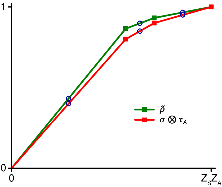
(g) Final state with the same $\beta$-ordering as $\sigma\otimes\tau_{A}$.

Figure 18: $\beta$-order change with Approximate Points Flows. In Step 1 of the protocol, APFs are performed so that the non-elbows of $\rho\otimes\tau_{A}$ can be horizontally aligned with the elbows of $\sigma\otimes\tau_{A}$. This transforms Figure (a) into Figure (b). In Step 2, PITRs are used to slightly misaligned the points in anticipation of Step 4. In this example they are misaligned to the right resulting in Figure (c). Next, PLTs are used in Step 3 to generate elbows (almost) horizontally aligned with those of $\sigma\otimes\tau_{A}$. This leads to Figure (d). Finally, in Step 4 APFs are applied to exactly match the elbows together with the non-elbow points. This is detailed in Figures (e) and (f). The result of the protocol is shown in Figure (g).

Appendix E Quantifying worst-case work costs with Crude Operations

Instead of using the wit construction summarized in Section A.3 to analyze the work value of a transformation, under Crude Operations one can consider the work value of the Level Transformations used during a process as defined in Eq. (14). In this section, we shall show that using this approach reproduces the results regarding worst-case work obtained under thermal operations in Horodecki and Oppenheim (2013); Åberg (2013).

E.1 Extractable work

By setting the final state to be $\tau_{S}$, the thermal state of the system, in Eq. (6), one can define the single-shot distillable work - the amount of work that can be obtained from a state. One can also consider the smoothed distillable work, where one allows the possibility of failing to distil positive work with some probability $\epsilon$. Denoting this quantity for a given state $\rho$ by $W^{\epsilon}_{\textrm{distil}}\left(\rho\right)$, in Horodecki and Oppenheim (2013); Åberg (2013) it was shown to be given by:

$$\begin{split}W^{\epsilon}_{\textrm{distil}}\left(\rho\right)&=F_{\textrm{min}}^{\epsilon}\left(\rho\right)+\frac{1}{\beta}\ln Z\\ &=-\frac{1}{\beta}\left[\ln\left(\tilde{L}_{1-\epsilon}\left(\rho\right)\right)-\ln Z\right],\end{split}$$ (37)

where $\tilde{L}_{y}$ denotes the horizontal distance between a state’s thermo-majorization curve and the $y$-axis at $y$, a quantity discussed more fully in Alhambra et al. (2015).

In Figure 19 we represent using thermo-majorization diagrams the protocol from Åberg (2013) that distills the amount of work given in Eq. (37). This protocol consists solely of Crude Operations. Note that as decohering is a Crude Operation which commutes with all other thermal operations Brandão et al. (2013), we can first decohere $\rho$ in the energy eigenbasis without altering the amount of work we can extract. Let $Z_{\epsilon}=\tilde{L}_{1-\epsilon}\left(\rho\right)$ denote the point on the $x$-axis such that those energy levels to the left of it on the thermo-majorization curve of $\rho$ have cumulative population given by $1-\epsilon$ and those energy levels to the right have total weight $\epsilon$. Without loss of generality, we can assume that $\left(Z_{\epsilon},1-\epsilon\right)$ is either an elbow or non-elbow on the thermo-majorization curve of $\rho$ as we can always make it so. To do this, we append a thermal qubit ancilla, $\tau_{A}$, consider the thermo-majorization curve of $\rho\otimes\tau_{A}$ and precede the extraction protocol with a Partial Isothermal Reversible Process to move a non-elbow to the desired location.

The protocol then runs as follows:

1. Raise the energy levels to the right of $Z_{\epsilon}$ to infinity using Level Transformations.

2. Fully thermalize the system.

3. Perform Partial Isothermal Reversible Processes to horizontally align the points on the system’s thermo-majorization curve with those of the target thermal state.

4. Perform a Level Transformation to transform the system into the thermal state of the initial Hamiltonian.

Two stages of this protocol have non-zero work value. The Level Transformation that takes Figure 19(a) to Figure 19(b) costs an infinitely large amount of work with probability $\epsilon$ and no work with probability $1-\epsilon$. The second Level Transformation that takes Figure 19(c) to Figure 19(d), has deterministic work yield $\frac{1}{\beta}\ln\left(\frac{Z}{Z_{\epsilon}}\right)$. Hence the overall protocol achieves the work value given in Eq. (37).

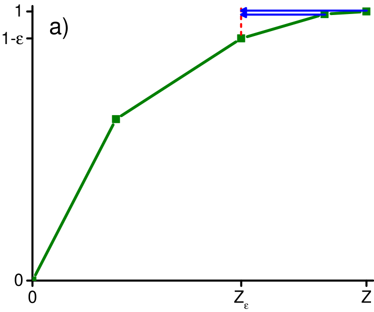
(a) LTs

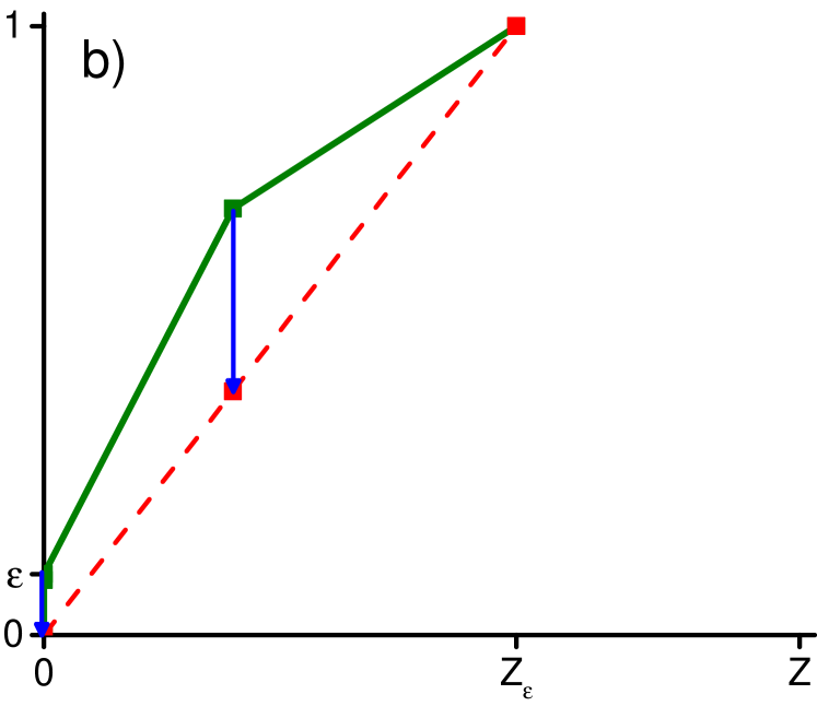
(b) PLTs

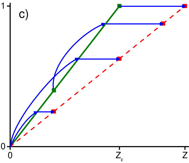
(c) PITRs and LTs

(d) Final state, $\tau$

Figure 19: Crude Operations protocol for $\epsilon$-deterministic work extraction. Here we illustrate the protocol for $\epsilon$-deterministic work extraction from Åberg (2013) in terms of thermo-majorization diagrams. First, the energy levels to the right of $Z_{\epsilon}$ are raised to infinity, transforming Figure (a) into Figure (b). Next, the system is fully thermalized, resulting in Figure (c). Finally, by applying PITRs and a deterministic LT, the system is transformed into the thermal state of the original Hamiltonian, Figure (d). Note that the first step, transforming Figure (a) into Figure (b), involves raising energy levels to infinity. This costs an infinitely large amount of work with probability $\epsilon$ and no work with probability $1-\epsilon$.

However, when this protocol fails, it fails spectacularly and costs an infinitely large amount of work. As discussed in Åberg (2013), this can be avoided if, rather than raising energy levels to infinity during the first Level Transformation, we instead raise them to a large but finite amount. However, this reduces the amount of work that is extracted when the protocol succeeds. The tradeoff between the cost of failure and the benefit of success is analyzed through the following protocol, illustrated in Figure 20.

Let $V$ denote the amount that we are willing to raise the energy levels to the right of $Z_{\epsilon}$ by (as we are raising energy levels, this will cost work). The protocol then runs as follows:

1. Raise the unoccupied energy levels to the right of $Z_{\epsilon}$ to infinity using Level Transformations.

2. Raise the occupied energy levels to the right of $Z_{\epsilon}$ by the amount $V$ using Level Transformations.

3. Fully thermalize the entire system.

4. Perform Partial Isothermal Reversible Processes to horizontally align the points on the system’s thermo-majorization curve with those of the target thermal state.

5. Perform a Level Transformation to transform the system into the thermal state of the initial Hamiltonian.

Again, two stages of this protocol have non-zero work value. The Level Transformation that takes Figure 20(a) to Figure 20(b) has work value $-V$ with probability $\epsilon$ and zero with probability $1-\epsilon$. The second Level Transformation that takes Figure 20(c) to Figure 20(d), has deterministic work yield $\frac{1}{\beta}\ln\left(\frac{Z}{Z_{\epsilon}+e^{-\beta V}\left(\tilde{L}_{1}\left(\rho\right)-Z_{\epsilon}\right)}\right)$. Hence, with probability $1-\epsilon$ the protocol produces a work value of:

$$\frac{1}{\beta}\ln\left(\frac{Z}{Z_{\epsilon}+e^{-\beta V}\left(\tilde{L}_{1}\left(\rho\right)-Z_{\epsilon}\right)}\right),$$ (38)

while with probability $\epsilon$ the work value is:

$$\frac{1}{\beta}\ln\left(\frac{Z}{Z_{\epsilon}+e^{\beta V}\left(\tilde{L}_{1}\left(\rho\right)-Z_{\epsilon}\right)}\right)-V.$$ (39)

As $V$ tends to infinity, we recover Eq. (37) while when $V=0$, the amount of work extracted is equal to $W^{0}_{\textrm{distil}}\left(\rho\right)$.

(a) LTs

(b) PLTs

(c) PITRs and LTs

(d) Final state, $\tau$

Figure 20: Crude Operations protocol for $\epsilon$-deterministic work extraction without infinite cost upon failure. Here we illustrate the protocol for $\epsilon$-deterministic work extraction without infinite work cost upon failure. First the energy levels to the right of $Z_{\epsilon}$ are raised by an amount $V$. The dotted red line in Figure (a) illustrates the effect of the Level Transformation on the thermo-majorization diagram and the higher the energy levels are raised, the steeper this line will be. In Figure (b), the resultant curve has been $\beta$-ordered, and this segment now lies between $y=0$ and $y=\epsilon$. Next the system is fully thermalized, resulting in Figure (c). Finally, by applying PITRs and a deterministic LT, the system is transformed into the thermal state of the original Hamiltonian, Figure (d). Note that this protocol produces less work when it succeeds than that described in Figure 19.

E.2 Work of formation

By setting the initial state to be $\tau_{S}$, the thermal state of the system, in Eq. (6), one can define the single-shot work of formation - the amount of work required to form a state without coherences. Denoting the work of formation for block-diagonal $\rho$ by $W_{\textrm{form}}\left(\rho\right)$, in Horodecki and Oppenheim (2013) it was shown to be given by:

$$\begin{split}W_{\textrm{form}}\left(\rho\right)&=-F_{\textrm{max}}\left(\rho\right)-\frac{1}{\beta}\ln Z_{S},\\ &=-\frac{1}{\beta}\left[\ln\left(\eta^{\left(\rho\right)}_{1}e^{\beta E_{1}^{\left(\rho\right)}}\right)+\ln Z_{S}\right],\end{split}$$ (40)

where the superscript $\left(\rho\right)$ again denotes that the occupation probabilities of $\rho$ and the associated energy levels of $H_{S}$ have been $\beta$-ordered.

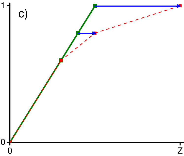
The protocol to form $\rho$ is illustrated in Figure 21 and runs as follows:

1. Partial Isothermal Reversible Processes are performed to transform $(\tau_{S},H_{S})$ into $(\rho,H^{\prime})$ where $H^{\prime}$ is such that $Z^{\prime}=Z_{S}$ and $\tau^{\prime}=\rho$.

2. All energy levels are raised by the same amount using a Level Transformation to form a curve that just thermo-majorizes that of the target state.

3. A second Level Transformation is performed to lower energy levels so as to match the energy levels of $H_{S}$.

As the first step consists of Partial Isothermal Reversible Processes, by Lemma 8 the work value of this step can be taken to be zero. Let the first Level Transformation be parametrized by $\mathcal{E}=\left\{h_{i}\right\}_{i=1}^{n}$ and the second Level Transformation by $\mathcal{E}^{\prime}=\left\{h^{\prime}_{i}\right\}_{i=1}^{n}$. Here:

$$h_{i} =\frac{1}{\beta}\left[\ln\left(\eta^{\left(\rho\right)}_{1}e^{\beta E_{1}^{\left(\rho\right)}}\right)+\ln Z_{S}\right],\quad\forall i,$$ (41)

$$h^{\prime}_{i} \leq 0,\quad\forall i.$$ (42)

Hence, using Eq. (14):

$$W_{\textrm{LT}_{\mathcal{E}}} =-\frac{1}{\beta}\left[\ln\left(\eta^{\left(\rho\right)}_{1}e^{\beta E_{1}^{\left(\rho\right)}}\right)+\ln Z_{S}\right],$$ (43)

$$W_{\textrm{LT}_{\mathcal{E}^{\prime}}} =0,$$ (44)

and the overall formation protocol has work cost given by Eq. (40).

(a) PITRs

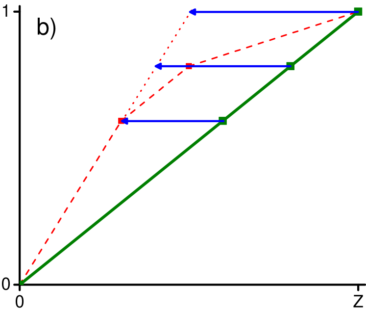
(b) LTs

(c) LTs

(d) Final state, $\rho$

Figure 21: Crude Operations protocol for state formation. Here we illustrate the protocol for state formation. First PITRs are applied to horizontally align the points of the initial state with those of $\rho$. This results in Figure (b). Next a LT is performed to raise the system’s energy levels and produce a curve that just thermo-majorizes the curve of $\rho$ as shown in Figure (c). This step costs work. Finally, energy levels are lowered where necessary using a LT to produce the final state, Figure (d). As energy levels are lowered, this final step does not cost work.

E.3 Work of transformation

Given two states, $\rho$ and $\sigma$, recall from Section A.3.1 that $W_{\rho\rightarrow\sigma}$ denotes the deterministic work required (if $W_{\rho\rightarrow\sigma}$ is negative) or gained (if $W_{\rho\rightarrow\sigma}$ is positive) in converting $\rho$ into $\sigma$ using thermal operations. This quantity can readily be obtained under Crude Operations. If one first performs the Level Transformation, $\textrm{LT}_{\mathcal{E}}$ with $\mathcal{E}=\left\{h_{i}=W_{\rho\rightarrow\sigma}\right\}_{i=1}^{n}$ to $\left(\rho,H_{S}\right)$ by definition, one is left with a system that thermo-majorizes $\left(\sigma,H_{S}\right)$. This system can now be converted into $\left(\sigma,H_{S}\right)$ using the protocol given in Theorem 13 and the work cost of the Level Transformation used is $W_{\rho\rightarrow\sigma}$.

Appendix F Crude Operations in the spirit of Szilard boxes

In this section we consider the case where the Hamiltonian is trivial, $H=0$, and we show how state-to-state transformations under Thermal Operation can be realized in the spirit of Szilard boxes with partitions (see, Figure 22). This provides a illustrative physical realization of $T$-transforms, while allowing one to quantify the work extracted in any process. This may give some readers a physical insight into previous sections. We will consider an arbitrary transformation, as well as work distillation and the work of formation.

The setup is as follows: we consider $d$ boxes (representing a $d$-level system), where each of the boxes has some probability $p_{i}$ ($i\in\left\{1,\ldots,d\right\}$) of finding a molecule in it. This is a realization of a density matrix $\rho=\sum p_{i}|i\rangle\langle i|$ and is general, since $H=0$. We can change the parameters of the boxes like volume and pressure, by adding a piston and letting it move in either directions or by temporarily removing and changing the placing of the walls of the boxes. We also assume we are able to shuffle the boxes to arrange the corresponding probabilities at no work cost.

Figure 22: A molecule in a box which is in contact with a thermal reservoir at temperature $T$. When we have many boxes, some probability of finding molecule in each of them is assigned. A piston can be added to change the pressure/volume or a wall can be moved to perform state transitions. The box can be used to describe the Szilard engine and the Maxwell demon thought experiment, where a piston is added to the box so that it is always pushed out by the molecule.

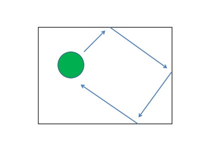
F.1 Work of distillation

Figure 23: Distillation with Szilard boxes. The probability of finding the molecule in one of the boxes marked with a green ball is at least $1-\epsilon$, which the empty boxes have a vanishingly small chance of being occupied. To distil work we first rearrange the boxes so that the unoccupied boxes are on the left, next we put in a piston and let it be pushed out to the right.

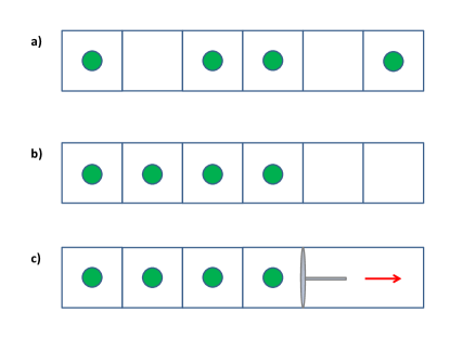
To distill work with probability at least $1-\epsilon$ as in Dahlsten et al. (2011), we first re-order of boxes, so they are arranged according to non-increasing probabilities of finding a molecule in it, $p_{i}$. Consider a situation when we have $d$ boxes, but most of the time, the molecule is found in one of $R$ of them (so that the probability of being in one of these $R$ boxes is at least $1-\epsilon$). The re-ordering ensures that the boxes which only have total probability at most $\epsilon$ of being occupied are on one side (let’s imagine it’s the right side). We then add a piston and let it be pushed out to the right thought the unoccupied boxes (for those $\sum p_{j}\leq\epsilon$). The work gain is due to the change of volume and is equal to $W=kT\operatorname{log\frac{V_{i}}{V_{f}}}=kT(\operatorname{log}d-\operatorname{log}R)$, where $kT$ is the product of the Boltzmann constant, $k$, and the temperature, $T$, and $V_{i}$, $V_{f}$, respectively the initial and final volume. In principle, the expression for work in proportion to the entropy change. We see, that it is non zero iff we have some ”unoccupied” boxes. Note that this extracts work with almost certainty (probability greater than $1-\epsilon$). One can obtain probabilistic work by inserting the piston between the first and second box, then the second and third, etc. Since once the boxes are re-ordered, the largest probabilities of being occupied are always on the left, the piston will be more likely to be pushed to the right, than to the left (which represents the loss of one bit of work).

F.2 Work of formation

Figure 24: State formation with Szilard boxes. In this example, we want to create the state which has probability $2/3$ of the molecule being on the left hand side, and $1/3$ of it being on the right, from a state where the molecule is uniformly distributed (the maximally mixed state). To do so, we push a piston in from the right, so that the volume available in the right hand partition is $1/3$ that of the left hand partition. We then insert a partition into the center and let the piston be pushed back out (which recovers the initial spent work with probability $1/3$.

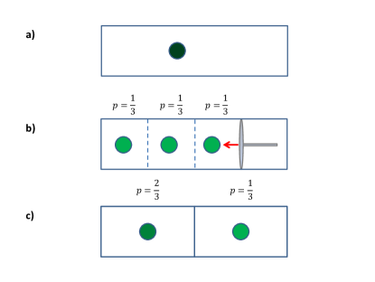
In Figure 24 we show how to form a state from the maximally mixed state with $d=2$. The larger the largest eigenvalue $\lambda$, the more the piston has to be pushed in, and it’s easy to see that the work required is $W=kT\operatorname{log\frac{V_{i}}{V_{f}}}=-kT\operatorname{log}\lambda$. This holds in higher dimension, since once the piston has been pushed in to create the largest eigenvalue, the majorization condition ensures that it can just be pushed back out, extracting work probabilistically in each step.

Note that we have irreversibility here. If we have no vacancies, i.e. unoccupied boxes, then the work of distillation is equal to 0, while the work of formation can be large, which means that we need to put energy in the system yet cannot get any from it.

F.3 Arbitrary transformations

An arbitrary transformation can be carried out much in the way of the cascade of T-transforms depicted in Figure 5. However, the method of moving probability mass is to insert a piston in place of the partition between two boxes, let the piston be moved out, and then replace the partitions. Namely, we once again arrange the boxes in non-increasing order, i.e. $p_{1}\geq p_{2}\geq p_{3}\geq\ldots\geq p_{d}$. We want to transform them into boxes with probabilities $q_{i}$ that are also in non-increasing order $q_{1}\geq q_{2}\geq q_{3}\geq\ldots\geq q_{d}$, assuming that p majorizes q. Then, initially, we have $p_{1}>q_{1}$. To adjust this probability we take the box with probability $p_{1}$, and replace it’s right partition wall with a piston. We then let the piston be pushed into the direction of the box with $p_{2}$ lowering the probability from $p_{1}$ to $q_{1}$ (if possible). The probability in the second box is now equal to $p_{1}+p_{2}-q_{1}>q_{2}$, which can be written as $p_{1}+p_{2}>q_{1}+q_{2}$, but it is already the majorization condition. We can repeat this process to arrange all boxes to transform the initial system into the final one.

References

- Scovil and Schulz-DuBois (1959) H. E. D. Scovil and E. O. Schulz-DuBois, Phys. Rev. Lett. 2, 262 (1959).
- Scully (2002) M. O. Scully, Phys. Rev. Lett. 88, 050602 (2002).
- Rousselet et al. (1994) J. Rousselet, L. Salome, A. Ajdari, and J. Prost, Nature 370, 446 (1994).
- Faucheux et al. (1995) L. P. Faucheux, L. S. Bourdieu, P. D. Kaplan, and A. J. Libchaber, Phys. Rev. Lett. 74, 1504 (1995).
- Baugh et al. (2005) J. Baugh, O. Moussa, C. Ryan, A. Nayak, and R. Laflamme, Nature 438, 470 (2005).
- Ruch and Mead (1976) E. Ruch and A. Mead, Theoretical Chemistry Accounts: Theory, Computation, and Modeling (Theoretica Chimica Acta) 41, 95 (1976).
- Horodecki and Oppenheim (2013) M. Horodecki and J. Oppenheim, Nature communications 4 (2013).
- Brandao et al. (2015) F. G. S. L. Brandao, M. Horodecki, N. H. Y. Ng, J. Oppenheim, and S. Wehner, Proc. Natl. Acad. Sci. 112, 3275 (2015).
- Note (1) Note that these generalized free energy constraints can be obtained from the thermo-majorization criteria provided one is allowed to use an ancillary system which is returned in its initial state at the end of protocol. As such, we can restrict ourselves to considering the thermo-majorization criteria here.
- Wilming et al. (2014) H. Wilming, R. Gallego, and J. Eisert, arXiv preprint arXiv:1411.3754 (2014).
- Janzing et al. (2000) D. Janzing, P. Wocjan, R. Zeier, R. Geiss, and T. Beth, International Journal of Theoretical Physics 39, 2717 (2000).
- Streater (1995) R. F. Streater, Statistical Dynamics: A Stochastic Approach to nonequilibrium Thermodynamics (Imperial College Press, London, UK, 1995).
- Brandão et al. (2013) F. G. S. L. Brandão, M. Horodecki, J. Oppenheim, J. M. Renes, and R. W. Spekkens, Phys. Rev. Lett. 111, 250404 (2013).
- Åberg (2014) J. Åberg, Phys. Rev. Lett. 113, 150402 (2014).
- Lostaglio et al. (2015) M. Lostaglio, K. Korzekwa, D. Jennings, and T. Rudolph, Phys. Rev. X 5, 021001 (2015).
- Ćwikliński et al. (2015) P. Ćwikliński, M. Studziński, M. Horodecki, and J. Oppenheim, Phys. Rev. Lett. 115, 210403 (2015).
- Åberg (2013) J. Åberg, Nature communications 4 (2013).
- Egloff et al. (2015) D. Egloff, O. Dahlsten, R. Renner, and V. Vedral, New Journal of Physics 17, 073001 (2015).
- Renes (2014) J. M. Renes, The European Physical Journal Plus 129, 1 (2014).
- Renes (2015) J. M. Renes, ArXiv e-prints (2015), arXiv:1510.03695 .
- Skrzypczyk et al. (2014) P. Skrzypczyk, A. J. Short, and S. Popescu, Nat. Commun. 5, 4185 (2014).
- Horodecki et al. (2003) M. Horodecki, P. Horodecki, and J. Oppenheim, Phys. Rev. A 67, 062104 (2003), quant-ph/0212019 .
- Muirhead (1902) R. F. Muirhead, Proceedings of the Edinburgh Mathematical Society 21, 144 (1902).
- Hardy et al. (1952) G. H. Hardy, J. E. Littlewood, and G. Pólya, Inequalities (Cambridge university press, 1952).
- Gour et al. (2015) G. Gour, M. P. Müller, V. Narasimhachar, R. W. Spekkens, and N. Yunger Halpern, Phys. Rep. 583, 1 (2015).
- Geusic et al. (1967) J. E. Geusic, E. O. Schulz-DuBios, and H. E. D. Scovil, Phys. Rev. 156, 343 (1967).
- Alicki (1979) R. Alicki, J. Phys. A: Math. Theor. 12, 0305 (1979).
- Gelbwaser-Klimovsky et al. (2013) D. Gelbwaser-Klimovsky, R. Alicki, and G. Kurizki, Phys. Rev. E 87, 012140 (2013).
- Howard (1997) J. Howard, Nature 389, 561 (1997).
- Geva and Kosloff (1992) E. Geva and R. Kosloff, The Journal of chemical physics 97, 4398 (1992).
- Hänggi and Marchesoni (2009) P. Hänggi and F. Marchesoni, Rev. Mod. Phys. 81, 387 (2009).
- Allahverdyan and Nieuwenhuizen (2000) A. E. Allahverdyan and T. M. Nieuwenhuizen, Phys. Rev. Lett. 85, 1799 (2000).
- Feldmann and Kosloff (2006) T. Feldmann and R. Kosloff, Phys. Rev. E 73, 025107 (2006).
- Linden et al. (2010) N. Linden, S. Popescu, and P. Skrzypczyk, Physical review letters 105, 130401 (2010).
- Dahlsten et al. (2011) O. Dahlsten, R. Renner, E. Rieper, and V. Vedral, New Journal of Physics 13, 053015 (2011).
- Del Rio et al. (2011) L. Del Rio, J. Åberg, R. Renner, O. Dahlsten, and V. Vedral, Nature 474, 61 (2011).
- Faist et al. (2012) P. Faist, F. Dupuis, J. Oppenheim, and R. Renner, arXiv preprint arXiv:1211.1037 (2012).
- Halpern and Renes (2014) N. Y. Halpern and J. M. Renes, arXiv preprint arXiv:1409.3998 (2014).
- Anders and Giovannetti (2013) J. Anders and V. Giovannetti, New Journal of Physics 15, 033022 (2013).
- Mueller and Pastena (2015) M. P. Mueller and M. Pastena, Phys. Rev. Lett. 115, 150402 (2015).
- Huber et al. (2015) M. Huber, M. Perarnau-Llobet, K. V. Hovhannisyan, P. Skrzypczyk, C. Klockl, N. Brunner, and A. Acin, New Journal of Physics 17, 065008 (2015).
- Narasimhachar and Gour (2015) V. Narasimhachar and G. Gour, Nature Communications 6, 7689 (2015).
- Alhambra et al. (2015) Á. M. Alhambra, J. Oppenheim, and C. Perry, arXiv preprint arXiv:1504.00020 (2015).
- Woods et al. (2015) M. P. Woods, N. Ng, and S. Wehner, ArXiv e-prints (2015), arXiv:1506.02322 .
- Lostaglio et al. (2015) M. Lostaglio, D. Jennings, and T. Rudolph, Nat. Commun. 6, 6383 (2015).
- Oppenheim (2013) J. Oppenheim, “Fundamental limitations for quantum and nano thermodynamics,” (2013), QIP talk.
- Marshall et al. (2010) A. W. Marshall, I. Olkin, and B. Arnold, Inequalities: theory of majorization and its applications (Springer Science & Business Media, 2010).