Effects of the tempered aging and its Fokker-Planck equation

Abstract

In the renewal processes, if the waiting time probability density function is a tempered power-law distribution, then the process displays a transition dynamics; and the transition time depends on the parameter $\lambda$ of the exponential cutoff. In this paper, we discuss the aging effects of the renewal process with the tempered power-law waiting time distribution. By using the aging renewal theory, the $p$-th moment of the number of renewal events $n_{a}(t_{a},t)$ in the interval $(t_{a},t_{a}+t)$ is obtained for both the weakly and strongly aged systems; and the corresponding surviving probabilities are also investigated. We then further analyze the tempered aging continuous time random walk and its Einstein relation, and the mean square displacement is attained. Moreover, the tempered aging diffusion equation is derived.

I Introduction

In 1975, Scher and Motroll Scher:1 used the continuous time random walk (CTRW) to study non-Gaussian anomalous diffusion. Nowadays, the CTRW model becomes popular in describing anomalous diffusion and a lot of chemical, physical, and biological processes Naftaly:1 ; Barkai:2 ; Barkai:6 , such as, the transport of electric charge in a complex system, diffusion in a low dimensional chaotic system, and the anomalous diffusion when cooling the mental solid and the twinkling of single quantum dot. In 1996, Monthusyx and Bouchaud introduce a CTRW framework for describing the aging phenomena in glasses Monthusyx:1 . This generalized CTRW is called aging continuous time random walk (ACTRW) in Barkai:1 . The complex dynamical systems displaying aging behaviour are quite extensive, including the fluorescence of single nanocrystals Brokmann:1 , aging effect in a single-particle trajectory averages Schulz:2 .

Research on statistics, based on power-law distributions with a heavy tail, yields many of significant results. Often the power-law distribution doesn’t extend indefinitely, due to the finite life span of particles, the boundedness of physical space. For this reason, in 1994, Mantegna and Stanley omit the large steps to study the truncated Lévy flights Mantegna:1 ; Negrete:1 . While the tempered power-law distribution Rosinski:1 uses a different approach, exponentially tempering the probability of large jumps. Exponential tempering offers technical advantages since the tempered process is still an infinitely divisible Lévy process which makes it convenient to identify the governing equation and compute the transition densities at any scale Baeumera:1 . By tempering, the distribution changes from heavy tail to semi-heavy, and the existence of conventional moments is ensured, which is useful in some practical applications. Recently tempered power-law distributions Meerschaert:1 have been observed for many geophysical processes at various scales Baeumera:1 ; Negrete:1 ; Sokolov:1 ; Meerschaert:2 ; Allegrini:1 , including interplanetary solar-wind velocity and magnetic field fluctuations measured in the alluvial aquifers Bruno:1 .

In this paper, we discuss the aging effects of the renewal processes with exponentially tempered power-law waiting time probability density function (PDF)

$$\varphi(t)=L_{\alpha}(t)e^{\lambda^{\alpha}-\lambda t}\sim\frac{1}{-\Gamma(-\alpha)}t^{-(1+\alpha)}e^{-\lambda t},$$ (1)

where $0<\alpha<1$, $L_{\alpha}(t)$ is the one side Lévy distribution Feller:1 ; levy:1 , and $\lambda>0$ is generally a small parameter. The semi-heavy tails and scale-free waiting time properties of $\varphi(t)$ play a particularly prominent role in diffusion phenomena.

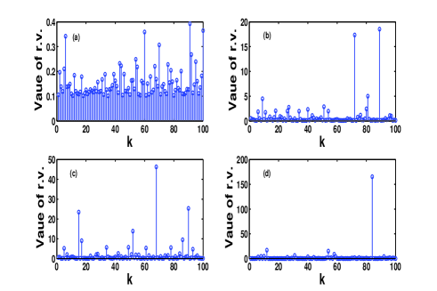
Figure 1: Random variables (r.v.) generated by Eq. (1) with $\alpha=0.6$. And the parameter $\lambda$ is chosen, respectively, as (a) $\lambda=10$, (b) $\lambda=10^{-1}$, (c) $\lambda=10^{-3}$, (d) $\lambda=10^{-5}$ and $k=1$, $2$, $\cdots$, 100.

From Eq. (1), it can be noted that if $0.1\ll t\ll 1/\lambda$, $\varphi(t)\sim t^{-(1+\alpha)}$, while if $t\gg 1/\lambda$, $\varphi(t)\sim\exp(-\lambda t)$. For the random variables generated by Eq. (1), Fig. 1 shows that the maximum and range of fluctuations vary dramatically with the change of $\lambda$. The introduced tempering forces the renewal process to converge from non-Gaussian to Gaussian. But the convergence is very slow, requiring a long time to find the trend. So, with the time passed by, both the non-Gaussian and Gaussian processes can be described.

This paper is organized as follows. In Sec. II, we use the aging renewal theory to obtain the $p$-th moment of the number of renewals $n_{a}(t_{a},t)$ within the time interval $(t_{a},t+t_{a})$ of the renewal process starting from time zero. The survival probability is, respectively, discussed in weakly and strongly aging system. We then turn to discuss the tempered ACTRW in Sec. III, and the mean square displacement is obtained for the cases $t_{a}\ll t$ and $t\ll t_{a}$. The numerical simulations confirm the analytical expressions of the mean square displacement. And the propagator function is also numerically obtained. In Sec. IV, we discuss the Einstein relation of the tempered ACTRW. The diffusion equation for the tempered ACTRW is derived in Sec. V, describing the time evolution of the PDF of the position. Finally, we conclude the paper with some remarks.

II Tempered aging renewal theory

First, we briefly outline the main ingredients in the CTRW and ACTRW. The standard CTRW assumes that the jumping transitions begin at time $t=0$, and observation of dynamics starts at $t_{a}$. The ACTRW modifies the statistic of time interval for first jump, namely, the waiting time PDF to the first jump is $\omega(t_{a},t)$. It describes a CTRW process having the aging time interval $(0,t_{a})$, while $t_{a}$ corresponding to the initial observation time $t=0$. Aging means that the number of renewals in the time interval $(t_{a},t_{a}+t)$ depends on the aging time $t_{a}$, even when the former is long. Thus generally ACTRW and CTRW exhibit different behaviors.

More concretely, ACTRW describes the following process: a walker is trapped on the origin for time $t_{1}$, then jumps to $x_{1}$; the walker is further trapped on $x_{1}$ for time $t_{2}$, and then jumps to a new position; this process is then renewed. Thus, ACTRW process is characterized by a set of waiting times $\{t_{1},t_{2},\cdots,t_{n},\cdots\}$ and displacements $\{x_{1},x_{2},\cdots,x_{n},\cdots\}$. Here $\omega(t_{a},t_{1})$ is the PDF of the first waiting time $t_{1}$. In ACTRW process, the random walk starts from the time $t_{a}$, therefore $\omega(t_{a},t_{1})$ may depend on the aging time of the process $t_{a}$. The waiting times ${t_{n}}$ with $n>1$ are independent and identically distributed (i.i.d.) with a common probability density $\varphi(t)$. And the jump lengths $\{x_{1},x_{2},\cdots,x_{n},\cdots\}$ are i.i.d. random variables, described by the probability density $f(x)$.

When $t_{a}=0$, we have $\omega(t_{a},t_{1})=\varphi(t_{1})$, which is just the well known Montroll-Weiss nonequilibrium process. In order to investigate ACTRW, we should first discuss the aging renewal process. In what follows, we suppose that $P_{n_{a}}(t_{a},t)$ is the probability of the renewal process $n_{a}(t_{a},t)$, where $n_{a}(t_{a},t)=n(t_{a}+t)-n(t)$ and $n(t)$ denotes the number of renewals by time $t$, i.e., $n_{a}(t_{a},t)$ is the number of renewals in time interval $(t_{a},t_{a}+t)$ for a precess starts at the time $0$. Our main work is to discuss the properties of the renewal process Luck:1 ; Schulz:1 in the time interval $(t_{a},t_{a}+t)$.

According to the renewal theory developed by Gordèche and Luck Luck:1 ,

$$\omega(s,u)=\frac{1}{1-\varphi(s)}\frac{\varphi(s)-\varphi(u)}{u-s},$$ (2)

where $\omega(s,u)$ is the double Laplace transform of the PDF of the first waiting time $\omega(t_{a},t_{1})$, and $\varphi(u)$ is the Laplace transform of $\varphi(t)$. This paper focuses on taking $\varphi(t)$ as Eq. (1), and its Laplace transform ($t\rightarrow u$) has the asymptotic form

$$\varphi(u)=e^{-(u+\lambda)^{\alpha}+\lambda^{\alpha}}\sim 1+\lambda^{\alpha}-(u+\lambda)^{\alpha},\indent 0<\alpha<1;$$ (3)

and if $\alpha=1$, $\varphi(u)\sim 1-u$.

The double Laplace transform of the PDF of $n_{a}(t_{a},t)$ reads Barkai:1 , $t_{a}\rightarrow s$, $t\rightarrow u$,

$$P_{n_{a}}(s,u)=\left\{\begin{array}[]{l@{\quad} l}\frac{1-s\omega(s,u)}{su},&n_{a}=0,\\ \\ \omega(s,u)\varphi^{n_{a}-1}(u)\frac{1-\varphi(u)}{u},&n_{a}\geq 1.\\ \end{array}\right.$$ (4)

For the particular case $\alpha=1$, from (3), $\omega(s,u)\sim 1/s$; and from Eq. (4) we can get $P_{n_{a}}(t_{a},t)\sim\delta(n_{a}-t)$, for this case $P_{n_{a}}(t_{a},t)$ is independent of $t_{a}$. Since $\omega(s,u)$ plays a key role in our discussion, we now derive the analytical formulation of $\omega(t_{a},t)$ Klafter:1 ,

$$\begin{split}\omega(s,t)&=\frac{1}{1-\varphi(s)}\exp(st)\int_{t}^{\infty}\exp(-sy)\varphi(y)dy\\ &\sim\frac{(s+\lambda)^{\alpha}}{\lambda^{\alpha}-(s+\lambda)^{\alpha}}\frac{\exp(st)}{\Gamma(-\alpha)}\Gamma(-\alpha,(s+\lambda)t),\end{split}$$ (5)

where $\Gamma(\alpha,x)=\int_{x}^{\infty}\exp(-t)t^{\alpha-1}dt$ is an incomplete Gamma function. Using the Laplace transform of incomplete Gamma function Oberhettinger:1 , we have,

$$\omega(t_{a},t)=\frac{\exp(-\lambda t)}{-\Gamma(-\alpha)}g(t_{a})*(\exp(-\lambda*t_{a})(t_{a}+t)^{-\alpha-1}),$$ (6)

where $g(t_{a})=t_{a}^{\alpha-1}\exp(-\lambda t_{a})E_{\alpha,\alpha}(\lambda^{\alpha}t_{a}^{\alpha})$. From the second line of Eq. (5), if $s\ll\lambda$, i.e., $t_{a}\gg 1/\lambda$. Eq. (5) can be given by

$$\omega(t_{a},t)\sim\frac{\lambda\exp(-\lambda t)\sin(\pi\alpha)}{\alpha\pi t^{\alpha}}\int_{0}^{t_{a}}\exp(-\lambda\tau)\frac{1}{\tau+t}\tau^{\alpha}d\tau.$$ (7)

If $s\gg\lambda$, i.e., $t_{a}\ll 1/\lambda$, then there exists $\frac{(s+\lambda)^{\alpha}}{(s+\lambda)^{\alpha}-\lambda^{\alpha}}\rightarrow 1$. Eq. (5) can be further simplified as

$$\omega(t_{a},t)\sim\frac{\sin(\pi\alpha)\exp(-\lambda(t+t_{a}))}{\pi}\frac{1}{t+t_{a}}\left(\frac{t_{a}}{t}\right)^{\alpha};$$ (8)

under the further assumption $t\ll 1/\lambda$, i.e., $\lambda t\ll 1$, there exists

$$\begin{split}\omega(t_{a},t)\sim&\frac{\sin(\pi\alpha)}{\pi}\frac{1}{t+t_{a}}\left(\frac{t_{a}}{t}\right)^{\alpha},\end{split}$$ (9)

being the same as the one given in Klafter:1 ; Barkai:1 for the power law waiting time, i.e., $\lambda=0$. When $\lambda$ is sufficiently large, Eq. (7) plays a dominant role.

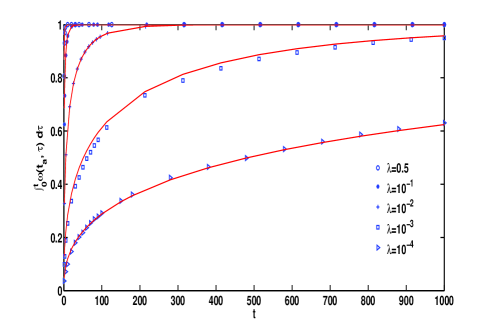
Figure 2: Probability of particles making jumps during the time interval $[t_{a},t_{a}+t]$ for $t_{a}\gg 1/\lambda$. The parameters of $\varphi(t)$ Eq. (1) are taken as $\alpha=0.6$, $t_{a}=10^{4}$, and $t=1000$; and the symboled lines are obtained by averaging $5000$ trajectories with different $\lambda$. The solid lines from down to up corresponding to the increased $\lambda$ are the theoretical results of Eq. (6). When $\lambda$ is large, the probability reaches $1$ quickly.

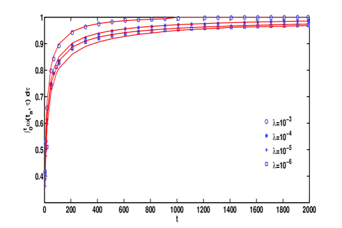
Figure 3: Probability of particles making jumps during the time interval $[t_{a},t_{a}+t]$. The parameters are taken as $\alpha=0.6$, $t_{a}=100$, and $t=2000$; and the symboled lines are obtained by averaging $5000$ trajectories with different $\lambda$. The solid lines from down to up corresponding to the increased $\lambda$ are the theoretical results of Eq. (6). When $\lambda$ is sufficiently small, the distribution is almost the same as pure power law for short times.

In the following, we analyze the asymptotic form of $\omega(t_{a},t)$ with $\alpha\in(0,1)$. From Eq. (2) and Eq. (3), there exists

$$\omega(s,u)\sim\frac{(s+\lambda)^{\alpha}-(u+\lambda)^{\alpha}}{(u-s)[\lambda^{\alpha}-(s+\lambda)^{\alpha}]}.$$ (10)

For Eq. (10), taking the limit $s\rightarrow\infty$, we have $\omega(s,u)\sim s^{-1}$; then $\omega(0,t)\sim\delta(t)$. Using the relation $P_{0}(t_{a},t)=1-\int_{0}^{t}\omega(t_{a},t)dt$ leads to $P_{0}(0,t)=0$, i.e., all the particles move at time $t=0$, no aging phenomenon.

Consider the survival probability $P_{0}(t_{a},t)$ krusemann:3 , which gives the probability of making no jumps during the interval $t_{a}$ up to $t_{a}+t$,

$$P_{0}(s,u)\sim\frac{1}{su}-\frac{(s+\lambda)^{\alpha}-(u+\lambda)^{\alpha}}{u(u-s)[\lambda^{\alpha}-(s+\lambda)^{\alpha}]}.$$ (11)

It is instructive to consider two different limits. If $s\ll u$, i.e., $t_{a}\gg t$, there exists

$$P_{0}(s,u)\sim\frac{1}{su}-\frac{(u+\lambda)^{\alpha}-\lambda^{\alpha}}{u^{2}[(s+\lambda)^{\alpha}-\lambda^{\alpha}]}.$$ (12)

For $\lambda\ll u$, i.e., $t_{0}\ll t\ll 1/\lambda$, then $(u+\lambda)^{\alpha}\sim u^{\alpha}(1+\lambda/u)^{\alpha}\sim u^{\alpha}$. Performing double inverse Laplace transform on the above equation results in

$$\begin{split}P_{0}(t_{a},t)\sim&\,1-t_{a}^{\alpha-1}\exp(-\lambda t_{a})E_{\alpha,\alpha}(\lambda^{\alpha}t_{a}^{\alpha})\Big{(}-\lambda^{\alpha}t\\ &+\frac{t^{1-\alpha}}{\Gamma(2-\alpha)}\Big{)}.\end{split}$$ (13)

For $t_{a}\ll 1/\lambda$, Eq. (13) can be simplified as

$$P_{0}(t_{a},t)\sim 1-t_{a}^{\alpha-1}\Big{(}-\lambda^{\alpha}t+\frac{t^{1-\alpha}}{\Gamma(2-\alpha)}\Big{)}.$$ (14)

It can be noted that $t^{1-\alpha}/\Gamma(2-\alpha)$ is larger than $\lambda^{\alpha}t$ in the parenthesis of Eq. (14), since $\lambda^{\alpha}t=(\lambda t)^{\alpha}t^{1-\alpha}\ll t^{1-\alpha}$. For $t_{a}\gg 1/\lambda$, from Eq. (13) and Eq. (69), we obtain

$$P_{0}(t_{a},t)\sim 1-\frac{t^{1-\alpha}}{\langle\tau\rangle\Gamma(2-\alpha)},$$ (15)

being confirmed by FIG. 4, i.e., the lines tend to be close for big $t_{a}$.

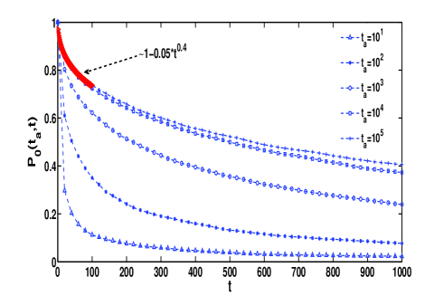
Figure 4: Time evolution of $P_{0}(t_{a},t)$ with different $t_{a}$. The parameters are taken as $\alpha=0.6$, $\lambda=10^{-4}$, and $t=1000$. The lines are obtained by averaging $5000$ trajectories. The (red) dashed line, $1-0.05*t^{0.4}$, is the fitting result for small $t$ and big $t_{a}$, which agrees with Eq. (15).

And for $t\ll t_{a}\ll 1/\lambda$, we have $P_{0}(t_{a},t)\sim 1$, i.e., for small $\lambda$, $\varphi(t)\sim t^{-1-\alpha}$, the waiting time is generally long; in a small observation time $t$, we cannot find movement of the particles. Eq. (11) can also be rewritten as

$$P_{0}(s,u)\sim\frac{1}{su}+\frac{1}{u(u-s)}+\frac{(u+\lambda)^{\alpha}-\lambda^{\alpha}}{u(s-u)[(s+\lambda)^{\alpha}-\lambda^{\alpha}]}.$$ (16)

For the case $u\ll s$, i.e., $t_{a}\ll t$, Eq. (16) yields

$$P_{0}(s,u)\sim\frac{(u+\lambda)^{\alpha}-\lambda^{\alpha}}{us[(s+\lambda)^{\alpha}-\lambda^{\alpha}]};$$ (17)

under the further assumption $u\gg\lambda$, we have

$$P_{0}(t_{a},t)\sim 1*g(t_{a})\frac{t^{-\alpha}}{\Gamma(1-\alpha)},$$ (18)

where $g(t_{a})$ is defined in Eq. (68), i.e., when $t_{a}\ll t\ll 1/\lambda$,

$$P_{0}(t_{a},t)\sim\frac{\sin(\pi\alpha)}{\pi\alpha}\left(\frac{t}{t_{a}}\right)^{-\alpha},$$ (19)

being the same as the result given in Luck:1 for the pure power law case ($\lambda=0$).

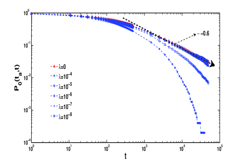
Figure 5: Time evolution of $P_{0}(t_{a},t)$ with different $\lambda$. The parameters are taken as $\alpha=0.6$, $t_{a}=500$, and $t=50000$. The lines are obtained by averaging $5000$ trajectories. The dashed line with arrow is for the indicator of slope $-0.6$, confirming Eq. (19).

When the aging time is sufficiently long relative to the observation time and $\lambda$ is small, the probability of making no jumps during the time interval $(t_{a},t_{a}+t)$ approaches to one, i.e., the system is completely trapped. On the contrary, if $t_{a}$ is short, while the observation time is long enough, then the particles are unacted on the aging time. So, at least one jump will be made, namely, the possibility of making no jumps is zero. Indeed, from Eq. (19), it can be easily obtained that $P_{0}(t_{a},t)\sim 0$ when $t/t_{a}\rightarrow\infty$; and $P_{0}(t_{a},t)\sim 0$ can also be directly obtained from Eq. (11) under the assumption $t\gg t_{a}$.

From Eq. (4), we can write the double Laplace transform of the PDF of $n_{a}(t_{a},t)$ as

$$P_{n_{a}}(s,u)=\frac{\delta(n_{a})}{u}\left[\frac{1}{s}-\omega(s,u)\right]+\omega(s,u)\varphi^{n_{a}-1}(u)\frac{1-\varphi(u)}{u}.$$ (20)

Inserting Eq. (3) into the above equation yields

$$\begin{split}P_{n_{a}}(s,u)\sim&~{}\omega(s,u)\exp^{-n_{a}[(u+\lambda)^{\alpha}-\lambda^{\alpha}]}\frac{(u+\lambda)^{\alpha}-\lambda^{\alpha}}{u}\\ &+\frac{\delta(n_{a})}{u}\left[\frac{1}{s}-\omega(s,u)\right].\end{split}$$ (21)

From now on, we start to calculate the $p$-th moment of the aging renewal process $n_{a}(t_{a},t)$ note:1 , which reads

$$\langle n_{a}^{p}(s,u)\rangle=\frac{\Gamma(p+1)\omega(s,u)}{u[(u+\lambda)^{\alpha}-\lambda^{\alpha}]^{p}}.$$ (22)

For the cases that $u\gg s$ and $\lambda\ll u$ or $u\ll s$, there exist

$$\langle n_{a}^{p}(s,u)\rangle\sim\left\{\begin{array}[]{ll}\frac{\Gamma(p+1)}{((s+\lambda)^{\alpha}-\lambda^{\alpha})u^{2+\alpha(p-1)}},&\hbox{for }s\ll u,\\ &~{}~{}~{}~{}\lambda\ll u;\\ \frac{\Gamma(p+1)}{(\alpha\lambda^{\alpha-1})^{p}}\frac{1}{su^{1+p}},&\hbox{for }u\ll s.\end{array}\right.$$ (23)

By double inverse Laplace transform we have

$$\langle n_{a}^{p}(t_{a},t)\rangle\sim\left\{\begin{array}[]{ll}\frac{\Gamma(p+1)}{\Gamma(2+\alpha p-\alpha)}g(t_{a})t^{\alpha p-\alpha+1},&\hbox{for }t\ll t_{a},\\ &~{}~{}~{}~{}\lambda t\ll 1;\\ (\frac{t}{\langle\tau\rangle})^{p},&\hbox{for }t_{a}\ll t.\end{array}\right.$$ (24)

Taking $p=1$ in (22) leads to

$$\langle n_{a}(s,u)\rangle=\frac{(s+\lambda)^{\alpha}-(u+\lambda)^{\alpha}}{u(u-s)[\lambda^{\alpha}-(s+\lambda)^{\alpha}][(u+\lambda)^{\alpha}-\lambda^{\alpha}]},$$ (25)

which can be rewritten as

$$\langle n_{a}(s,u)\rangle=\frac{1}{u(s-u)}\left(\frac{1}{(u+\lambda)^{\alpha}-\lambda^{\alpha}}-\frac{1}{(s+\lambda)^{\alpha}-\lambda^{\alpha}}\right).$$ (26)

We will confirm that if both $t_{a}$ and $t$ are large scales, $\langle n_{a}(t_{a},t)\rangle\sim t/\langle\tau\rangle$, which is an important result for normal diffusion. For small $u$ and $s$, using the Taylor expansion $(u+\lambda)^{\alpha}\sim\lambda^{\alpha}+\alpha\lambda^{\alpha-1}u$ and $(s+\lambda)^{\alpha}\sim\lambda^{\alpha}+\alpha\lambda^{\alpha-1}s$, from Eq. (26), we have

$$\langle n_{a}(s,u)\rangle\sim\frac{1}{\alpha\lambda^{\alpha-1}u^{2}s}.$$ (27)

Performing double Laplace transform on the above equation yields

$$\langle n_{a}(t_{a},t)\rangle\sim\frac{t}{\alpha\lambda^{\alpha-1}}=\frac{t}{\langle\tau\rangle},$$ (28)

where $\langle\tau\rangle=\alpha\lambda^{\alpha-1}$ (see Appendix C).

For the slightly aging system, $t\gg t_{a}$, i.e., $u\ll s$; performing the double inverse Laplace transform on both sides of (26) yields

$$\begin{split}\langle n_{a}(t_{a},t)\rangle\sim&(t^{\alpha-1}e^{-\lambda t}E_{\alpha,\alpha}(\lambda^{\alpha}t^{\alpha}))*1\\ &-(t_{a}^{\alpha-1}e^{-\lambda t_{a}}E_{\alpha,\alpha}(\lambda^{\alpha}t_{a}^{\alpha}))*1\\ \sim&(t^{\alpha-1}e^{-\lambda t}E_{\alpha,\alpha}(\lambda^{\alpha}t^{\alpha}))*1.\end{split}$$ (29)

For the special case, $\lambda=0$, it can be noted that $\langle n_{a}(t_{a},t)\rangle\sim t^{\alpha}$. For $t\gg 1/\lambda$, using the asymptotic expansion of Mittag-Leffler function (66), from Eq. (29), we again obtain $\langle n_{a}(t_{a},t)\rangle\sim\frac{t}{\langle\tau\rangle}$. In the long time scale, the process converges to the Gaussian process, and then the first moment of the number of renewal events grows linearly with the observation time $t$. For $t\ll 1/\lambda$, from Eq. (29) we have

$$\langle n_{a}(t_{a},t)\rangle\sim\frac{1}{\Gamma(1+\alpha)}t^{\alpha}.$$ (30)

It can be seen that when $t\gg t_{a}$ the first moment of $n_{a}$ is not relevant to the aging time $t_{a}$. From Eq. (28) and Eq. (30), we can see that $\lambda$ plays an important role in our discussion as expected.

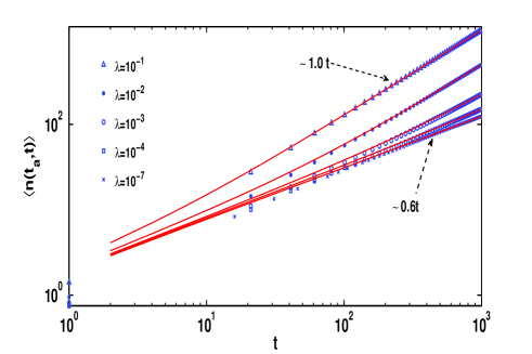
Figure 6: Time evolution of the ensemble average of the renewal times $\langle n_{a}(t_{a},t)\rangle$ with the waiting time PDF Eq. (1) for slight aging. The parameters are taken as $\alpha=0.6$, $t_{a}=3$, and $t=1000$. The real lines are for the analytical result Eq. (29) and the other lines are obtained by averaging $5000$ trajectories.

While for the strongly aging system, $t_{a}\gg t$, i.e., $s\ll u$; there exists

$$\langle n_{a}(s,u)\rangle\sim\frac{1}{u^{2}[(s+\lambda)^{\alpha}-\lambda^{\alpha}]},$$ (31)

which yields

$$\langle n_{a}(t_{a},t)\rangle\sim tt_{a}^{\alpha-1}e^{-\lambda t_{a}}E_{\alpha,\alpha}(\lambda^{\alpha}t_{a}^{\alpha}).$$ (32)

Following the way used above, for $t_{a}\gg 1/\lambda$, the term $t_{a}^{\alpha-1}E_{\alpha,\alpha}(\lambda^{\alpha}t_{a}^{\alpha})e^{-\lambda t_{a}}$ tends to $\lambda^{1-\alpha}/\alpha$ (69). Then we have

$$\langle n_{a}(t_{a},t)\rangle\sim\frac{t}{\langle\tau\rangle}.$$ (33)

For $t_{a}\ll 1/\lambda$, there exists Luck:1 ; Klafter:1

$$\langle n_{a}(t_{a},t)\rangle\sim\frac{1}{\Gamma(\alpha)}tt_{a}^{\alpha-1}.$$ (34)

The above results for the first moment of $n_{a}(t_{a},t)$ can be summarized as: 1. if $t_{a}$ or $t$ is greater than $1/\lambda$, then $\langle n_{a}(t_{a},t)\rangle\sim t/\langle\tau\rangle$; 2. for $t\gg t_{a}$ and $t\ll 1/\lambda$ (i.e. $t^{-\alpha-1}\exp(-\lambda t)\sim t^{-\alpha-1}$), $\langle n_{a}(t_{a},t)\rangle\sim t^{\alpha}/\alpha$; 3. for $t\ll t_{a}$ and $t_{a}\ll 1/\lambda$, $\langle n_{a}(t_{a},t)\rangle$ behaves as $tt_{a}^{\alpha-1}$.

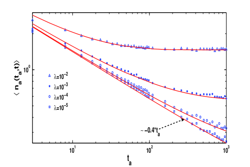
Figure 7: The relation between the $\langle n_{a}(t_{a},t)\rangle$ and $\lambda$ for $t_{a}\gg t$ according to the trajectories and the theory. The number of particles is $3000$, $t_{a}=1000$, $t=5$ , $\alpha=0.6$, and $\lambda=10^{-2}$, $10^{-3}$, $10^{-4}$, and $10^{-5}$. The real lines are for the analytical result Eq. (32) and the other symbol lines are obtained by averaging $5000$ trajectories.

Figure 8: Time evolution of the ensemble average of the renewal times $\langle n_{a}(t_{a},t)\rangle$ for strong aging ($t_{a}\gg t$). The parameters $\alpha=0.6$, $t_{a}=1000$, and $\lambda=10^{-1}$ for (a); $\lambda=10^{-2}$ for (b); $\lambda=10^{-3}$ for (c); $\lambda=10^{-4}$ for (d). The lines are obtained by averaging $10^{4}$ trajectories. It can be seen that $\langle n_{a}(t_{a},t)\rangle$ grows linearly with time $t$ for fixed $t_{a}$ for all values of $\lambda$, which confirms the analytical result Eq. (32).

III Tempered ACTRW

III.1 Mean squared displacement

After understanding the statistics of the number of renewals, we go further to discuss the tempered ACTRW with the waiting time distribution Eq. (1). The process of ACTRW has been described in Sec. II. This paper focuses on the symmetric random walk, i.e., the distribution of jump lengths $f(x)=f(-x)$; and $M_{2}=\int_{-\infty}^{+\infty}x^{2}f(x)dx$ is finite. For such a random walk, we denote $P(x,t_{a},t)$ as the PDF of particles’ position in the decoupled tempered ACTRW with aging time $t_{a}$. Then

$$P(x,t_{a},t)=\sum^{\infty}_{n_{a}=0}P_{n_{a}}(t_{a},t)f_{n_{a}}(x),$$ (35)

where $P_{n_{a}}(t_{a},t)$ means the probability of jumping $n_{a}$ steps in the time interval $(t_{a},t_{a}+t)$, and $f_{n_{a}}(x)$ the probability of jumping to the position $x$ after $n_{a}$ steps. In the Fourier-Laplace domain,

$$P(k,s,u)=\sum^{\infty}_{n_{a}=0}P_{n_{a}}(s,u)f^{n_{a}}(k).$$ (36)

Inserting Eq. (4) into Eq. (36) leads to

$$P(k,s,u)=\frac{1-s\omega(s,u)}{su}+\frac{\omega(s,u)(1-\varphi(u))}{u}\frac{f(k)}{1-\varphi(u)f(k)}.$$ (37)

By differentiating Eq. (37) two times with respect to $k$ and setting $k=0$, we derive the second order moment of the random walks, i.e.,

$$\langle r^{2}(s,u)\rangle=\frac{\omega(s,u)M_{2}}{u[1-\varphi(u)]}.$$ (38)

For the mean square displacement, we present the results of the slightly aging and strongly aging system, i.e.,

$$\langle r^{2}(s,u)\rangle\sim\left\{\begin{array}[]{l@{\quad} l}\frac{M_{2}}{us[(u+\lambda)^{\alpha}-\lambda^{\alpha}]},&\hbox{for }u\ll s,\\ \\ \frac{M_{2}}{u^{2}[(s+\lambda)^{\alpha}-\lambda^{\alpha}]},&\hbox{for }u\gg s.\\ \end{array}\right.$$ (39)

Performing double inverse Laplace transform on $\langle r^{2}(s,u)\rangle$ yields

$$\langle r^{2}(t_{a},t)\rangle\sim\left\{\begin{array}[]{l@{\quad} l}M_{2}g(t)*1,&\hbox{for }t\gg t_{a},\\ \\ M_{2}tg(t_{a}),&\hbox{for }t_{a}\gg t,\\ \end{array}\right.$$ (40)

where $g(z)=z^{\alpha-1}\exp(-\lambda z)E_{\alpha,\alpha}(\lambda^{\alpha}z^{\alpha})$.

From FIG. (10), we can see the large fluctuations of $\langle r^{2}(t_{a},t)\rangle$ even if the number of trajectories is 10000. This is because that most of particles are trapped in the initial position for $t_{a}\gg t\ll 1/\lambda$, which is consistent with Eq. (13). This is related to population splitting Cherstvya:1 .

It can be noted that when $t\gg t_{a}$, the mean squared displacement has no aging effect; while $t\ll t_{a}$ ($\lambda t_{a}\ll 1$), it is deeply affected by the aging time $t_{a}$. The surprising result is that $\langle r^{2}(t_{a},t)\rangle\sim\langle n_{a}(t_{a},t)\rangle$, when the second order moment of the jump length is finite; the same things happen for the pure power-law waiting time distribution.

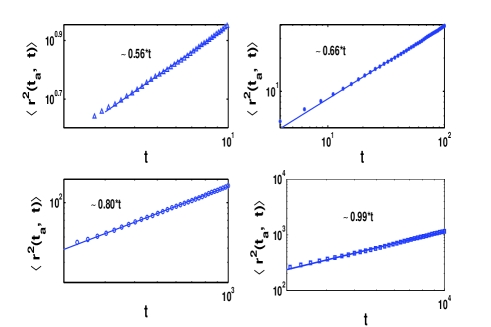
Figure 9: The relation between the $\langle r^{2}(t_{a},t)\rangle$ and the observation time $t$ for $t_{a}\ll t$ getting from the trajectories of the particles (dashed line) and Eq. (40) (real line). The parameters $\alpha=0.6$, $\lambda=10^{-3},$ $t_{a}=1$, and the number of trajectories is $5000$. With the increase of $\lambda$, the characteristic of $\langle r^{2}(t_{a},t)\rangle$ changes from Power law to normal diffusion.

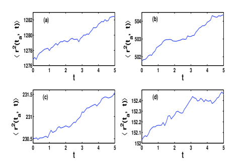
Figure 10: The relation between $\langle r^{2}(t_{a},t)\rangle$ and the observation time $t$ for $t_{a}\gg t$. It can be noted that $\langle r^{2}(t_{a},t)\rangle$ increases linearly with $t$ for fixed $t_{a}$ and the fluctuations are large because of population splitting. The parameter $t_{a}=1000$, $t=5$, $\lambda=10^{-1}$ for (a), $\lambda=10^{-2}$ for (b), $\lambda=10^{-3}$ for (c), $\lambda=10^{-4}$ for (d), $\alpha=0.6$ and the number of the trajectories is $10000$.

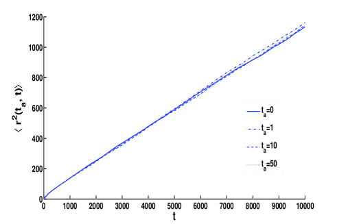
Figure 11: The relation between $\langle r^{2}(t_{a},t)\rangle$ and the observation time $t$ for various $t_{a}$ with $t\gg t_{a}$.

III.2 Propagator function $P(x,t_{a},t)$

In this subsection, we discuss the propagator function $P(x,t_{a},t)$ of the tempered ACTRW. Omitting the motionless part of Eq. (37), taking $f(x)$ as Gaussian, and performing inverse Fourier transform w.r.t. $k$, there exists

$$P(x,s,u)\sim\frac{\omega(s,u)}{2u}F_{1}(u,x)$$ (41)

with

$$\begin{split}F_{1}(u,x)=&\sqrt{\frac{(u+\lambda)^{\alpha}-\lambda^{\alpha}}{0.5(1+\lambda^{\alpha}-(u+\lambda)^{\alpha})}}\\ &\cdot\exp\left(-|x|\sqrt{\frac{(u+\lambda)^{\alpha}-\lambda^{\alpha}}{0.5(1+\lambda^{\alpha}-(u+\lambda)^{\alpha})}}\right).\end{split}$$

For $u\ll s$, Eq. (41) can be rewritten as

$$P(x,t_{a},u)\sim\left(\frac{\lambda^{\alpha}-(u+\lambda)^{\alpha}}{2u}[g(t_{a})*1]+1\right)F_{1}(u,x).$$ (42)

From FIG. (12), it can be noted that for small $\lambda$ ($\lambda=10^{-3}$ or $\lambda=10^{-4}$) the propagator functions display the characteristics of $\alpha$ stable distribution; while for large $\lambda$ the $P(x,t_{a},t)$ shows the classical normal behavior.

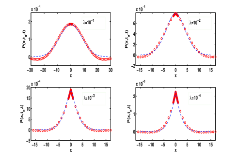
Figure 12: Propagator functions with $t_{a}=3$, $\alpha=0.6$, and $t=500$. The red lines with empty symbol are obtained by calculating Eq. (42), and the blue dash lines are got from the generated $10^{4}$ trajectories of the particles.

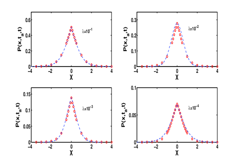
Figure 13: Strong aging case (contrary to FIG. (12)) with $t_{a}=500$ and $t=3$. The other parameters are same as FIG. (12).

For $u\gg s$, Eq. (37) yields,

$$P(x,t_{a},u)\sim\frac{(u+\lambda)^{\alpha}-\lambda^{\alpha}}{2u^{2}}g(t_{a})F_{1}(u,x).$$ (43)

Contrary to FIG. (12), FIG. (13) displays the behaviors of the $\alpha$ stable distribution for all kinds of $\lambda$.

From the numerical results and the theory we can see that the ‘$\alpha$ stable distribution’ characteristics can be found for small $\lambda$. Both the distributions for $\lambda=10^{-3}$ and $\lambda=10^{-4}$ have the sharp peak and the tail of Eq. (42) decays slowly. While for large $\lambda$, the top of the distribution for Eq. (42) is smooth, being different from the case of small $\lambda$. Therefore, depending on the choice of $\lambda$, one can control the behaviors of the propagator.

IV strong relation between the fluctuation and response

In this section, we discuss the aging from a new point of view. Based on the CTRW model, consider such a process: the particles begin to move at time $t=0$ and undergo unbiased diffusion in the time interval $(0,t_{a})$; then an external field is switched on the system starting from $t_{a}$. If the averaged response of the particles depends on $t_{a}$, the process is said to exhibit aging. Generally speaking, giving some disturbance to a system, some characteristics (parameters of thermodynamics) of the system will change, being called response Bertin:1 . Under the small disturbance of external field, if the change of the parameter of thermodynamics is proportional to the force of external field, then it is called linear response. It seems important to use drift diffusion to consider aging. Using the method given in Barkai:7 ; Allegrini:3 ; Froemberg:1 ; Shemer:1 , we discuss the tempered aging Einstein relation.

Let us consider a simple example of random walk on a one-dimensional lattice; the length of the lattice is $c$, and the particles can only move to its neighboring sites. Waiting times of different steps of the random walk are considered independent and have the same distribution $\psi(t)$. Jumps to the right (left) are performed with the probability $1/2+h/2$ ($1/2-h/2$). The total time is $t=t_{a}+t_{b}$; $[0,t_{a}]$ is called aging interval with $h=0$; and $(t_{a},t_{a}+t_{b})$ is called response interval with $0<h<1$. Let $x=x_{a}+x_{b}$, where $x_{a}=\sum_{i=1}^{n_{a}}x_{i}^{a}$ is the displacement performed in the aging time interval and $x_{b}=\sum_{i=1}^{n_{b}}x_{i}^{b}$ is the displacement performed in the response time interval, and $x_{i}^{a},x_{i}^{b}$ are the step lengths and $n_{a},n_{b}$ are the number of events happened in the two time intervals, repectively.

We consider the correlation function $\langle(x_{a})^{2}x_{b}\rangle$ which shows the impact between $(x_{a})^{2}$ in the aging interval and $x_{b}$ in the response interval. And define a parameter $F_{R}$ to show the relation between fluctuation and response Barkai:7 ,

$$F_{R}=\frac{\langle(x_{a})^{2}x_{b}\rangle}{\langle(x_{a})^{2}\rangle\langle x_{b}\rangle}-1.$$ (44)

If $F_{R}=0$, it shows that $x_{a}^{2}$ and $x_{b}$ are independent with each other. Using the relation $\langle x_{a}^{2}\rangle=c^{2}\langle n_{a}\rangle$ and $\langle x_{b}\rangle=hc\langle n_{b}\rangle$, then $F_{R}$ can be shown in another way,

$$F_{R}=\frac{\langle n_{a}n_{b}\rangle}{\langle n_{a}\rangle\langle n_{b}\rangle}-1.$$ (45)

We further introduce $X_{t_{a},t_{b}}(n_{a},n_{b})$, the probability to occur $n_{a}$ events in the aging interval and $n_{b}$ events in the response interval. Following the result given in Luck:1 ,

$$\begin{split}X_{t_{a},t_{b}}(n_{a},n_{b})&=\langle I(t_{n_{a}}<t_{a}<t_{n_{a}+1})\\ &I(t_{n_{a}+n_{b}}<t_{a}+t_{b}<t_{n_{a}+n_{b}+1})\rangle,\end{split}$$ (46)

where $I(t_{n_{a}}<t_{a}<t_{n_{a}+1})=1$ if the event inside the parenthesis occurs, and $0$ if not. Using double Laplace transform, if $n_{b}=0$,

$$X_{s,u}(n_{a},n_{b})=\frac{\varphi^{n_{a}}(s)}{u}\left[\frac{1-\varphi(s)}{s}-\frac{\varphi(u)-\varphi(s)}{s-u}\right];$$ (47)

and if $n_{b}\geq 1$,

$$X_{s,u}(n_{a},n_{b})=\frac{\varphi^{n_{a}(s)}\psi^{n_{b}-1}(u)}{u(s-u)}[1-\varphi(u)][\varphi(u)-\varphi(s)].$$

Summing $n_{a}$, $n_{b}$ from $0$ to $\infty$ leads to

$$\langle n_{a}n_{b}\rangle_{s,u}=\frac{[\varphi(u)-\varphi(s)]\varphi(s)}{u(s-u)(1-\varphi(s))^{2}(1-\varphi(u))}.$$

Using the Laplace transform of $\varphi(t)$ (3), we have, when $t_{a}\gg t_{b}$,

$$\begin{split}\langle n_{a}n_{b}\rangle_{t_{a},t_{b}}\sim&\,t_{b}[t_{a}^{\alpha-1}E_{\alpha,\alpha}(\lambda^{\alpha}t_{a}^{\alpha})\exp(-\lambda t_{a})]\\ &*[t_{a}^{\alpha-1}E_{\alpha,\alpha}(\lambda^{\alpha}t_{a}^{\alpha})\exp(-\lambda t_{a})];\end{split}$$ (48)

if $t_{a}\ll t_{b}$, there exists

$$\begin{split}\langle n_{a}n_{b}\rangle_{t_{a},t_{b}}\sim&(1*[t_{a}^{\alpha-1}E_{\alpha,\alpha}(\lambda^{\alpha}t_{a}^{\alpha})\exp(-\lambda t_{a})])\\ &\cdot(1*[t_{b}^{\alpha-1}E_{\alpha,\alpha}(\lambda^{\alpha}t_{b}^{\alpha})\exp(-\lambda t_{b})])\\ &-1*[t_{a}^{\alpha-1}E_{\alpha,\alpha}(\lambda^{\alpha}t_{a}^{\alpha})\exp(-\lambda t_{a})]\\ &*[t_{a}^{\alpha-1}E_{\alpha,\alpha}(\lambda^{\alpha}t_{a}^{\alpha})\exp(-\lambda t_{a})].\end{split}$$ (49)

Following the results given by Luck:1 ,

$$\langle n_{a}\rangle_{s,u}=\frac{\varphi(s)}{us(1-\varphi(s))},$$

there exists

$$\langle n_{a}\rangle_{t_{a},t_{b}}=(1*[t_{a}^{\alpha-1}E_{\alpha,\alpha}(\lambda^{\alpha}t_{a}^{\alpha})\exp(-\lambda t_{a})]).$$ (50)

And $\langle n_{b}\rangle_{s,u}$ is the same as Eq. (25). For $t_{a}\gg t_{b}$, there exists

$$F_{R}(t_{a},t_{b})\sim\frac{[t_{a}^{\alpha-1}E_{\alpha,\alpha}(\lambda^{\alpha}t_{a}^{\alpha})\exp(-\lambda t_{a})]*[t_{a}^{\alpha-1}E_{\alpha,\alpha}(\lambda^{\alpha}t_{a}^{\alpha})\exp(-\lambda t_{a})]}{(1*[t_{a}^{\alpha-1}E_{\alpha,\alpha}(\lambda^{\alpha}t_{a}^{\alpha})\exp(-\lambda t_{a})])t_{a}^{\alpha-1}E_{\alpha,\alpha}(\lambda^{\alpha}t_{a}^{\alpha})\exp(-\lambda t_{a})}.$$ (51)

From Eq. (51), we know that $F_{R}(t_{a},t_{b})$ does depend on $t_{b}$.

In the following, we further consider the Einstein relation Froemberg:1 ; Shemer:1 for the tempered aging process. Denoting $\langle x(t_{a},t_{b})\rangle_{F}$ as the first order moment of the displacement under the influence of a force $F$, from Eq. (32) and $\langle x(t_{a},t_{b})\rangle_{F}=hc\langle n_{b}\rangle$, we get that for $t_{a}\gg t_{b}$,

$$\langle x(t_{a},t_{b})\rangle_{F}\sim hct_{b}t_{a}^{\alpha-1}E_{\alpha,\alpha}(\lambda^{\alpha}t^{\alpha}_{a})\exp(-\lambda t_{a}).$$ (52)

Denoting $\langle r^{2}(t_{a},t_{b})\rangle_{0}$ as the mean squared displacement of the random walk without external force, from Eq. (40) we obtain that for $t_{a}\gg t_{b}$,

$$\langle r^{2}(t_{a},t_{b})\rangle_{0}\sim M_{2}t_{b}t_{a}^{\alpha-1}E_{\alpha,\alpha}(\lambda^{\alpha}t^{\alpha}_{a})\exp(-\lambda t_{a})$$ (53)

with $M_{2}=1/2c^{2}+1/2(-c)^{2}=c^{2}$. Under the assumption $h=\frac{cF}{2K_{b}T}\ll 1$, we obtain the following relation,

$$\langle x(t_{a},t_{b})\rangle_{F}\sim\frac{F}{2K_{b}T}\langle r^{2}(t_{a},t_{b})\rangle_{0}.$$ (54)

V Fokker-Planck equation for the tempered ACTRW

We now derive the Fokker-Planck equation of the tempered ACTRW, which can be used to solve the tempered aging diffusion problems with different types of boundary and initial condition. Omitting the motionless part of Eq. (37) and taking $f(x)$ as Gaussian (i.e., $f(k)\sim 1-\frac{1}{2}k^{2}$), we have

$$\begin{array}[]{l}P(k,s,u)\\ \displaystyle\sim\frac{\omega(s,u)}{u}\frac{(u+\lambda)^{\alpha}-\lambda^{\alpha}}{(u+\lambda)^{\alpha}-\lambda^{\alpha}+\frac{1}{2}k^{2}(1+\lambda^{\alpha}-(u+\lambda)^{\alpha})}.\end{array}$$ (55)

Define the Riemann-Liouville fractional derivative from $0$ to $t$ as,

$$_{0}D_{t}^{p}y(t)=\frac{1}{\Gamma(n-p)}\frac{d^{n}}{dt^{n}}\int_{0}^{t}(t-\tau)^{n-p-1}y(\tau)d\tau,$$ (56)

where $n=[p]+1$ and $[\,]$ denotes the integer part of $p$. For $0<p<1$, taking the Laplace transform of the Riemann-Liouville fractional derivative results in

$$\mathcal{L}[{{}_{0}D_{t}^{p}y(t)}]=s^{p}\mathcal{L}[y(t)]=s^{p}y(s).$$ (57)

From the property of the inverse Fourier transform, we have

$$\mathcal{F}^{-1}[k^{2}y(k)]=-\frac{\partial^{2}}{\partial x^{2}}y(x).$$ (58)

From Eq. (57) and Eq. (58), performing once inverse Fourier transform and double inverse Laplace transforms leads to

$$\begin{split}&-e^{-\lambda t}~{}_{0}D_{t}^{\alpha}\left(e^{\lambda t}P(x,t_{a},t)\right)+\lambda^{\alpha}P(x,t_{a},t)\\ =&-\frac{1}{2}(1+\lambda^{\alpha})\frac{\partial^{2}}{\partial x^{2}}P(x,t_{a},t)+e^{-\lambda t}{{}_{0}D_{t}^{\alpha}}\left(e^{\lambda t}\frac{\partial^{2}}{\partial x^{2}}P(x,t_{a},t)\right)\\ &+\lambda^{\alpha}[\omega(t_{a},t)\ast 1]\delta(x)-[1\ast e^{-\lambda t}{{}_{0}D_{t}^{\alpha}}\left(e^{\lambda t}\omega(t_{a},t)\right)]\delta(x),\end{split}$$ (59)

where the notation $\ast$ represents the convolution of the functions w.r.t. $t$. Eq. (59) is the Fokker-Planck equation of the Green function $P(x,t_{a},t)$ in the case that the waiting time distribution is the tempered power-law (1).

For the non tempered case, namely, $\lambda=0$ and $\varphi(t)\sim t^{-1-\alpha}$, taking $\lambda=0$ in Eq. (55) results in

$$P(k,s,u)\sim\omega(s,u)\frac{u^{\alpha-1}}{u^{\alpha}+\frac{k^{2}}{2}(1-u^{\alpha})}.$$ (60)

Performing inverse Fourier transform and double inverse Laplace transform on Eq. (57) yields the corresponding aging diffusion equation

$$\begin{split}{}_{0}D_{t}^{\alpha}P(x,t_{a},t)=&\frac{1}{2}\frac{\partial^{2}}{\partial x^{2}}P(x,t_{a},t)-{{}_{0}D}_{t}^{\alpha}\frac{\partial^{2}}{\partial x^{2}}P(x,t_{a},t)\\ &-\omega(t_{a},t)\ast\frac{t^{-\alpha}}{\Gamma(1-\alpha)}\delta(x).\end{split}$$ (61)

As expected, taking $\lambda=0$ in Eq. (59) also arrives at Eq. (61). There are also other forms of Eq. (59), e.g., adding the motionless part of (37) to the equation; for the longer time scale $t\gg 1$, then $u^{\alpha}k^{2}$ can be reasonably omitted Barkai:5 , i.e., the term ${}_{0}D_{t}^{\alpha}\frac{\partial^{2}}{\partial x^{2}}P(x,t_{a},t)$ can be omitted in Eq. (61).

VI Conclusions

Because of the boundedness of physical space and the finiteness of the lifetime of particles, sometimes it is a more physical choice to use tempered power-law jump length or waiting time distribution instead of the pure power-law distribution. This paper discusses the renewal process and ACTRW with the tempered power-law waiting time distribution $\varphi(t)\sim e^{-\lambda t}t^{-1-\alpha}$. Since the tempered power-law distribution lies between the pure power-law and exponential distributions, as expected, the transition dynamics is found with the time evolution and the turning point depends on $\lambda$. By using the aging renewal theory, the $p$-th moments of the renewal times $n_{a}(t_{a},t)$ are analytically obtained and numerically confirmed by simulating the particles’ trajectories. In particular, the first order moment of $n_{a}(t_{a},t)$ is more detailedly discussed. Similarly, the mean squared displacement of the tempered ACTRW is analytically got and numerically verified. Based on the $p$-th moment of $n_{a}(t_{a},t)$ and mean squared displacement of the tempered ACTRW, the aging effects are deeply analyzed. Finally, the tempered aging Einstein relation is attained and the corresponding Fokker-Planck equation is derived from the tempered ACTRW.

Appendix A Generation of random variables (FIG. 1)

When generating the random variables with the PDF Eq. (1) to plot FIG. 1, the Monte Carlo statistical methods Christain:1 is used. We first rewrite $\varphi(t)$ as $\varphi(t)=H(x)f_{1}(x)$, where $f_{1}(x)=\alpha t_{0}^{\alpha}t^{-\alpha-1}$ with $t_{0}$ being a small number. Denote the maximum of $H(x)$ as $M$. Then the algorithm can be described as:

1. Generate a r.v. $x_{f_{1}}$ with PDF $f_{1}$ and a r.v. $\xi$ being uniformly distributed in the interval $[0,1]$.

2. Accept $x_{f_{1}}$, if $M\xi\leq H(x_{f_{1}})$; otherwise, reject.

3. Return to Step $1$.

Appendix B Mittag-Leffler function

The two-parameter function of the Mittag-Leffler type plays a very important role in the fractional calculus, being introduced by G.M. Mittag-Leffler and studied by A. Wiman podlubny:1 . The two-parameter Mittag-Leffler function is defined by the series expansion

$$E_{\alpha,\beta}=\sum_{k=0}^{\infty}\frac{z^{k}}{\Gamma(\alpha k+\beta)}$$ (62)

with $\alpha>0$ and $\beta>0$. Its one-parameter form ($\beta=1$) is given as

$$E_{\alpha}=\sum_{k=0}^{\infty}\frac{z^{k}}{\Gamma(\alpha k+1)}.$$ (63)

The asymptotic expansions of Mittag-Leffler are important for obtaining the various useful estimates of the long time or short time fractional dynamics. For small $z$, there exists

$$E_{\alpha,\beta}(z)\sim\frac{1}{\Gamma(\beta)}+\frac{z}{\Gamma(\alpha+\beta)},$$ (64)

in the special case, $E_{\alpha}(z)\sim 1+\frac{z}{\Gamma(\alpha+1)}$. Another important and useful formula is the asymptotic expansion of large scale for the Mittag-Leffler function. For $0<\alpha<2$, $\beta$ is an arbitrary complex number and $\mu$ is an arbitrary real number such that $\pi\alpha/2<\mu<\min\{\pi,\pi\alpha\}$, then for an arbitrary integer $p\geq 1$, the following expansion holds,

$$\begin{split}E_{\alpha,\beta}(z)\sim&\frac{1}{\alpha}z^{(1-\beta)/\alpha}\exp(z^{1/\alpha})\\ &-\sum_{k=1}^{p}\frac{z^{-k}}{\Gamma(\beta-\alpha k)}\end{split}$$ (65)

with $z\rightarrow\infty$ and $\arg(z)\leq\mu$. For $z\rightarrow+\infty$, from Eq. (65), we have

$$E_{\alpha,\beta}(z)\sim\frac{1}{\alpha}z^{(1-\beta)/\alpha}\exp(z^{1/\alpha}).$$ (66)

And if $z\rightarrow-\infty$,

$$E_{\alpha,\beta}(z)\sim-\frac{1}{z\Gamma(\beta-\alpha)}-\frac{1}{z^{2}\Gamma(\beta-2\alpha)};$$ (67)

when $\alpha=\beta$, we have $|\Gamma(0)|\rightarrow\infty$. Therefore $E_{\alpha,\alpha}(z)\sim-\frac{1}{z^{2}\Gamma(-\alpha)}$.

In the analysis of this paper, we use the following function several times.

$$g(z)=z^{\alpha-1}\exp(-\lambda z)E_{\alpha,\alpha}(\lambda^{\alpha}z^{\alpha}).$$ (68)

When $z\rightarrow+\infty$, from (66), there exists

$$g(z)\sim\frac{\lambda^{1-\alpha}}{\alpha};$$ (69)

see Fig. 14.

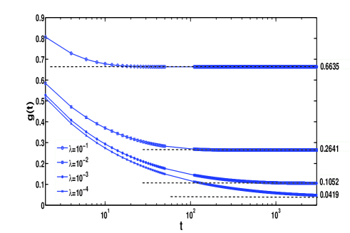
Figure 14: Time evolution of $g(t)$.

While for $z\rightarrow 0$, from (64), we have $g(z)\sim 1/\Gamma(\alpha)z^{\alpha-1}$.

Appendix C Laplace transform of $\varphi(t)$

Here we present the Laplace transform of Eq. (1). From the definition of the survival probability on a site, i.e., the probability that the waiting time on a site exceeds $t$,

$$\Psi(t)=\int_{t}^{\infty}\varphi(\tau)d\tau=1-\int_{0}^{t}\varphi(\tau)d\tau.$$ (70)

Using the definition of incomplete Gamma function, for Eq. (1) we have

$$\begin{split}\Psi(t)&\sim\lambda^{\alpha}\int_{\lambda t}^{\infty}\exp(-z)z^{-\alpha-1}dz\\ &=\lambda^{\alpha}\Gamma(-\alpha,\lambda t).\end{split}$$ (71)

According to the Laplace transform of the incomplete Gamma function $\mathcal{L}[\Gamma(-\alpha,\lambda t)]=\Gamma(-\alpha)[1-(\frac{u+\lambda}{\lambda})^{\alpha}]/u$ with $\Re e(-\alpha)>-1$ and $\Psi(t)$, we have

$$\psi(u)\sim 1+\lambda^{\alpha}-(u+\lambda)^{\alpha}.$$ (72)

From Eq. (72), we have two useful asymptotics. For the long time scale, $t\gg 1/\lambda$, (i.e., $u\ll\lambda$) by the Taylor expansion, we have

$$\psi(u)\sim 1-\alpha\lambda^{\alpha-1}u+\alpha(1-\alpha)\lambda^{\alpha-2}u^{2}+\cdots+(-1)^{n+1}(-\alpha)(1-\alpha)\cdots((n-1)-\alpha)\lambda^{\alpha-n}u^{n}.$$ (73)

Notice that $\psi(0)=1$, so the PDF is normalized. From the definition of $\langle\tau^{n}\rangle=\int_{0}^{\infty}\tau^{n}\psi(\tau)d\tau$, we can get $\langle\tau\rangle=\alpha\lambda^{\alpha-1}$, and $\langle\tau^{2}\rangle=(1-\alpha)(-\alpha)\lambda^{\alpha-2}$. For the general cases, $\langle\tau^{n}\rangle=-\Gamma(n-\alpha)/\Gamma(-\alpha)\lambda^{\alpha-n}$, i.e., $\psi(u)\sim 1-\langle\tau\rangle u+\langle\tau^{2}\rangle u^{2}+\cdots+(-1)^{n}\langle\tau^{n}\rangle u^{n}$. For short time scale, $t_{0}<<t\ll 1/\lambda$ (i.e. $u\gg\lambda$),, we have

$$\psi(u)\sim 1+u^{\alpha}\left[\left(\frac{\lambda}{u}\right)^{\alpha}-\left(1+\frac{\lambda}{u}\right)^{\alpha}\right]\sim 1-u^{\alpha}.$$ (74)

References

- (1) H. Scher and E.W. Montroll, Phys. Rev. B 12, 2455 (1975).
- (2) A. Naftaly, Y. Edery, I. Dror,and B. Berkowitz, J. Hazard. Mater.bf 299 513 (2015).
- (3) E. Barkai, R. Metzler, and J. Klafter, Phys. Rev. E 61, 132 (2000).
- (4) E. Barkai, Chem. Phys. 284, 13 (2002).
- (5) C. Monthusyx and J. -P. Bouchaud, J. Phys. A: Math. Gen. 29, 3847 (1996).
- (6) E. Barkai and Y.-C. Cheng, J. Chem. Phys. 118, 6167 (2003).
- (7) X. Brokmann, J. P. Hermier, G. Messin, P. Desbiolles, J. P. Bouchaud, and M. Dahan, Phys. Rev. Lett. 90, 120601 (2003).
- (8) J. H. P. Schulz, E. Barkai, and R. Metzler, Phys. Rev. Lett. 110, 020602 (2013).
- (9) R. N. Mantegna and H. E. Stanley, Phys. Rev. Lett. 73, 2946 (1994).
- (10) D. del-Castillo-Negrete, Phys. Rev. E 79, 031120 (2009).
- (11) J. Rosiński, Stochastic Process. Appl. 117, 677 (2007).
- (12) B. Baeumera and M.M. Meerschaert, J. Comput. Appl. Math. 233, 2438 (2010).
- (13) M. M. Meerschaert, P. Roy and Q. Shao, Comm. Statist. Theory Methods 41, 1839 (2012).
- (14) I. M. Sokolov, A. V. Chechkin, and J. Klafter, Phys. A 336, 245 (2004).
- (15) M. M. Meerschaert, Y. Zhang, and B. Baeumer, Geophys. Res. Lett. 35, L17403 (2008).
- (16) P. Allegrini, G. Aquino, P. Grigolini, L. Palatella, and A. Rosa, Phys. Rev. E 68, 056123 (2003).
- (17) Bruno, R., L. Sorriso-Valvo, V. Carbone, and B. Bavassano, Europhys. Lett. 66, 146-152(2004)
- (18) W. Feller, An introduction to probability theory and its applications (wiley, New york, 1970). Vol. 2.
- (19) The one sided stable Lévy distribution in Laplace space can be conveniently expressed as, , for .
- (20) C. Godrèche and J. M. Luck, J. Stat. Phys. 104, 489 (2001).
- (21) J. H. P. Schulz, E. Barkai, and R. Metzler, Phys. Rev. X 4, 011028 (2014).
- (22) The moment of a probability distribution of with density is defined as,
- (23) J. Klafter and I. M. Sokolov, First Steps in Random Walks: From Tools to Applications (Oxford University Press, Oxford, 2011).
- (24) F. Oberhettinger and L. Baddi, Tables of Laplace Transform (Springer, Berlin, 1973).
- (25) A. G. Cherstvya and Ralf Metzler, Phys. Chem. Chem. Phys., 15, 20220 2013.
- (26) M. Bertin and J. -P. Bouchaud, Phys. Rev. E 67, 065105(R) (2003).
- (27) D. Froemberg and E. Barkai, Phys. Rev. E 87, 030104(R) (2013).
- (28) E. Barkai, Phys. Rev. E 75, 060104(R) (2007).
- (29) P. Allegrini, G. Aquino, P. Grigolini, L. Palatella, A. Rosa, and B.J. West, Phys. Rev. E,71, 066109 (2005).
- (30) Z. Shemer and E. Barkai, Phys. Rev. E 80, 031108 (2009).
- (31) C. P. Robert and G. Casella, Monte Carlo Statistical Methods (springer, New York, 2004).
- (32) I. Podlubny, Fractional Differntial Equations (Academic Press, New York, 1999).
- (33) E. Barkai, Phys. Rev. Lett. 90, 104101 (2003).
- (34) H. Krüsemann A. Godec, and R. Metzler, Phys. Rev. E 89, 040101(R) (2014).