Simulating central forces in the classroom

Abstract

We describe the easy to customize and extend open source Java program Central force workbench that can be used in the classroom to simulate the motion of a particle (or a two-body system) under central forces. It may be useful to illustrate problems in which the analytical solution is not available as well as to help students to grasp a more intuitive understanding of the main features of this kind of problem and to realize the exceptional nature of the particular case of Newtonian (and harmonic) forces. We also include some suggestions on how to use the program as a pedagogical tool.

I Introduction

When physics students are introduced to central forces the subject is mainly, if not exclusively, focused on Newtonian forces. While this is completely justified by the physical importance (and historical influence) of Newtonian forces, it is not always stressed the exceptional nature of this kind of force law among all the possible central forces. I have often found students that think any orbit of positive mechanical energy is hyperbolic, even if the force is not Newtonian. Of course, this belief can be dispelled by telling them that in a harmonic potential $V\propto r^{2}$ every orbit is elliptic and has positive energy. However, this in turn can reinforce a seemingly natural tendency to think that bounded orbits are always elliptic or, at least, closed, while it is a consequence of a dynamical symmetry bb:symmetry ; bb:mtnez ; bb:goldstein3 the closely related bb:grant Newtonian and harmonic force laws.

Even in the Newtonian case there is room for misunderstandings. When dealing with the two-body problem one is lead to separate the (trivial) motion of the center-of-mass and the relative motion of the two bodies. After studying the Keplerian orbits, many students are perplexed if asked how would look the orbit of each body in the center-of-mass system or, worse, in another inertial frame in which the total linear momentum is not null (as we should expect to see in the motion of a binary star system). This is clearly an instance in which a simulation may be helpful.

On the other hand, force laws for which there is a closed analytical solution for the orbit equation are exceptional (although of paramount importance): apart from the Newtonian and harmonic cases, one can mention the potential $V=-k/r+a/r^{2}\$bb:goldstein4 and the special relativistic version of the Kepler problem, bb:boyer which can be solved by using essentially the same computation needed for Newtonian forces. The Cotes’ spirals bb:Whittaker are even more remarkable because not only the orbit equation but also the time evolution may be solved by elementary methods. There are other cases in which the orbit equation can be solved in terms of special functions, bb:goldstein but they are of little use in introductory courses. Finally there is a handful of cases in which the solution (or, at least, the orbit equation) can be computed in terms of elementary functions for special values of the initial conditions (often when the mechanical energy vanishes or equals the maximum value of the effective potential).

For these reasons a versatile computational tool that can be easily used in the classroom (and by students at home) to simulate the motion under central forces can be a valuable pedagogical asset. The aim of this work is to present such a tool, which we will succinctly do in Section II, while Section III will be devoted to suggest how to effectively use it as a pedagogical tool in a introductory course on mechanics. The Appendix provides a complete reference for users of the program.

II The program

Central force workbench is written in the freeware platform Easy Java/Javascript Simulations by Francisco Esquembre. bb:paco A single file, central.jar, bb:jar contains everything: the executable code, the source code and the complete help system. It can be run as a standalone program in any computer with Java 1.5 or newer. The same file can also be embedded in a web page. bb:web The program is open source and the source code may be extracted from central.jar and easily extended and customized by means of Easy Java/Javascript Simulations, bb:paco which can also be used to add translations to other languages (the current distribution includes English and Spanish).

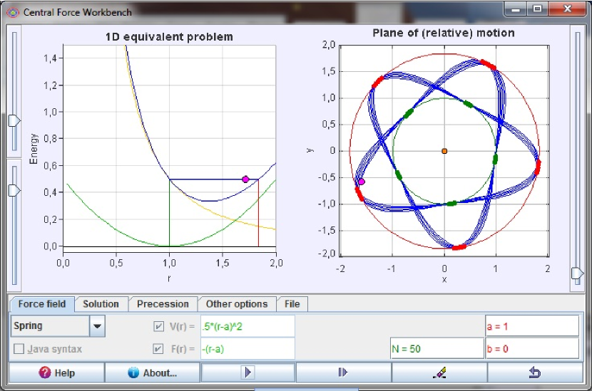
Figure 1: The main window of the simulation.

The main window, shown in Figure 1, displays on the left the potential $V(r)$ in green, the centrifugal term $L^{2}/2mr^{2}$ in orange and the effective potential $V_{\mathrm{e}}(r)\equiv V(r)+L^{2}/2mr^{2}$ in blue. ($L$ is the angular momentum and $m$ the particle mass or the reduced mass for the two-body system). There will appear the evolution in the equivalent one-dimensional problem corresponding to the radial motion. The two-dimensional motion of the single particle (or the relative motion in the two-body problem) is displayed on the right.

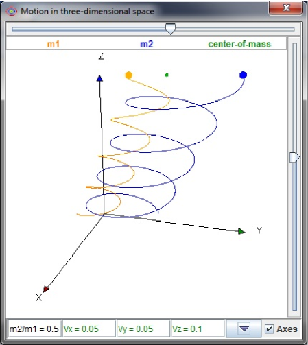
Figure 2: Three-dimensional projection of a two-body system evolution.

Optionally, a projection of the three-dimensional motion of both particles in the two-body problem can be seen in another windows (see Figure 2). There one can select the projection direction in either the center-of-mass system or in another inertial frame in which the center-of-mass moves with prescribed constant velocity.

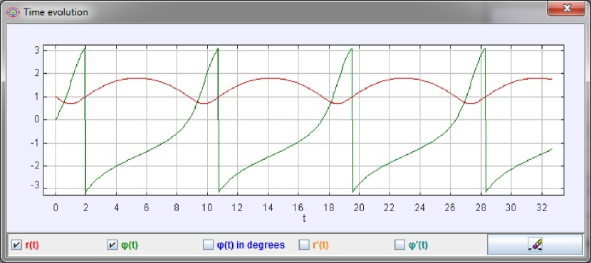
Figure 3: Time evolution of polar coordinates.

It is also possible to display the time evolution of the polar coordinates $r$ and $\varphi$ and their time derivatives, as shown in Figure 3. Furthermore, all the results displayed in the different windows can be captured in a video sequence or exported in several graphics formats, including Encapsulated PostScript. The solution points can also be exported in a numerical table and a tool to perform data analysis (including Fourier analysis) of the solution points is embedded in the program: just right click on an orbit and choose the appropriate menu entry.

The force law can be selected from a list of predefined examples, but the user is free to enter its own law or to modify one of the predefined ones. Physical parameters (initial conditions, energy, angular momentum and parameters in the force law), options for the numerical code (integration method and tolerance) and display settings can be easily changed. It is also possible to make the program display and compute the orbit apses, in order to compute precession, for instance. The program is user-friendly (an informative tooltip is displayed when the mouse hovers over an element) and includes a complete help system, with a troubleshooting section.

We refer the interested reader to the Appendix (or to the help system) for more information on using the program.

III Suggested activities

The simulation provides a general framework to explore motion in central force fields. By selecting User defined in the Force field tab the user may define its own problem, maybe starting from one of the predefined ones. We list below the predefined force fields, which we have used in the classroom, in the form of exercises to be solved by means of the program and, in some cases, by using analytical methods. After a short formulation of each exercise, we add a short comment. (In the examples included in the program the units are chosen so that $k=m=GM=1$.)

Newtonian

: “Simulate the Keplerian orbits, in the potential $V(r)=-k/r$, for different values of the mechanical energy $E$ and angular momentum $L$. Consider both the attractive case ($k>0$) and the repulsive force ($k<0$).”
Comment: The program can be useful for illustration purposes.

Harmonic

: “Check that every orbit in the harmonic potential $V(r)=\frac{1}{2}kr^{2}$ is elliptic if $k>0$. Discuss the difference between these elliptic orbits and the Newtonian ones. Which among Kepler’s laws are still satisfied and how do we have to change the remaining? What happens if $k<0$?”
Comment: As mentioned before, this can be used to stress that positive mechanical energy does not imply hyperbolic orbits. The simulation may be also used instead of a formal proof of the elliptic nature of the orbits.

Bertrand

: “Check that among the potentials in the form $V(r)=kr^{a}$ only in the Newtonian case $a=-1$ and in the harmonic case, $a=2$, all bounded orbits are closed (i.e., periodic). You may try $a=-1,\ -1.02,\ -0.98,\ 2.02,\ldots$ Try finding isolated periodic orbits (the Precession tab may be useful when using trial and error to do this).”
Comment: This can be used to introduce precession and, especially, to discuss Bertrand’s theorem. bb:bertrand ; bb:brown ; bb:goldstein2 Students should realize the exceptional nature of Newtonian and harmonic forces, where a dynamical symmetry (the Laplace-Runge-Lenz vector or the equivalent Hamilton eccentricity vector) makes closed every bounded orbit. bb:symmetry ; bb:mtnez ; bb:goldstein3

Spring

: “A point mass moves on a smooth table, attached to a spring of proper length $a$. Show that the mass moves in the central potential $V(r)=\frac{1}{2}k(r-a)^{2}$. Compute some orbits. Try finding periodic orbits.”
Comment: Another modification of the harmonic force which gives very different orbits (see Figure 1). This is a simple example in which the force is both attractive and repulsive along many orbits.

Constant force

: “A particle sliding without friction inside a vertical conical surface, or two particles connected by a string passing through a small hole in a horizontal smooth table). Show that the particle moves in the central potential $V(r)=kr$, for appropriate $k$. Try finding periodic orbits, including circular ones.”
Comment: A couple of equivalent well known examples. bb:amalio ; bb:sacks

Galaxy

: “In a naive model of the motion of a star around a galaxy of radius $R$, total mass $M$ and constant density, the force for $r\leq R$ is harmonic, $F(r)=-GMmr/R^{3}$, and for $r\geq R$ Newtonian, $F(r)=-GMm/r^{2}$. Check that the orbits are periodic ellipses if they are inside the radius $R$ and, in general open if they cross that value.”
Comment: A mix of harmonic and Newtonian cases, bb:jiang which again shows the exceptionality of those cases.

Yukawa

: “Discuss, in terms of the angular momentum $L$, the existence and stability of circular orbits in the Yukawa potential $V(r)=-k\exp(-r/a)/r$ from nuclear physics.”
Comment: An illustration of unstable circular orbits.

Ion-atom

: “Check that in the potential $V(r)=-k/r^{4}$ for the ion-atom interaction, the orbits with energy $E=0$ are circles of radius $(km/2L^{2})^{1/2}$ going through the force center. Which is the maximum impact parameter $b=L/(2mE)^{1/2}$ for capture? Discuss the orbits with $E=L^{4}/16km^{2}$: find their analytical expression.”
Comment: The simplest case of circular orbit with the geometric center outside the force center (the remaining cases are discussed in bb:petsch ). The strong singularity at $r=0$ provides an opportunity to discuss difficulties in numerical simulations.

Cotes

: “Find the orbit equation $r(\varphi)$ and the time evolution, $(r(t),\varphi(t))$, of a particle moving in the potential $V(r)=-k/r^{2}$.”
Comment: Everything can be calculated in terms of elementary functions. The orbits a called Cotes’ spirals. bb:Whittaker

Open orbits

: “Check that orbits in the potential $V(r)=-k/r+a/r^{2}$, with $a>-L^{2}/2m$ with negative energy are periodic (i.e., closed) when $a=L^{2}(p^{2}/q^{2}-1)/2m$, for $p,\ q=1,2,\ldots$ These orbits have $p$ pericenters (and $p$ apocenters) every $q$ turns around the force center (or the other particle in two-body problems). Use the Precession tab to check the analytic result for precession: $\Delta\varphi=2\pi[(1+2ma/L^{2})^{-1/2}-1]$.”
Comment: This is an interesting example because a full analytical solution for the orbit equation is easy to obtain, bb:goldstein4 which gives exact values for precession and existence of closed orbits.

Precession

: “The potential $V(r)=-a/r(1+b/r^{2})$, with $a=GMm$ and $b=L^{2}/m^{2}c^{2}$, describes the motion of a test particle in a static gravitational field with spherical symmetry (i.e., in the Schwarzschild metric). bb:hobson1 Since for Mercury (for instance) $b$ is very small, the general relativistic contribution to the perihelion precession is easier to compute by analytical (approximate) methods. However, one can use the simulation for periastron precessions in strong gravitational fields (i.e., for $b$ not so small). Use the Precession tab to check the analytic (approximate) result for precession: $\Delta\varphi\approx 6\pi m^{2}a^{2}b/L^{4}$. Notice that in this case $t$ is the proper time along the particle worldline.”
Comment: An illustration from General Relativity.

Light

: “The potential $V(r)=-a/r^{3}$ , with $a=GMh^{2}/c^{2}$, describes the motion of a photon in a static gravitational field with spherical symmetry (the Schwarzschild metric). bb:hobson2 Here $t$ is the affine parameter and $h=r^{2}d\varphi/dt$ a conserved quantity. The light deviation by the Sun is too small: you’d better use a not so small value for $a$. Use the Precession tab to check the analytic (approximate) result for light deviation: $\Phi\approx 4GM/bc^{2}$, where $b$ is the impact parameter. In our notation $m=1$, $h=L=b(2E)^{1/2}$ and $\Phi\approx 4a(2E)^{1/2}/L^{3}$.”
Comment: The second example from General Relativity.

IV Conclusions

We have presented a versatile, portable, customizable and free program that can be a useful resource for teaching central forces. Some ideas to effectively use the tool in the classroom have been included.

Appendix: Program reference

This appendix has been taken from the help system and can be skipped on first reading, but it might be useful to fully appreciate the many features in the program.

IV.1 Description of the program

This simulation explores the motion of a particle (or a two-body system) in a central potential $V(r)$. The user can select the latter from a number of built-in examples or define a new one.

• The unit mass is the particle mass (or the reduced mass for the two-body problem), so that $m=1$.

• At the bottom of the main window there is a panel with five tabs. In Force field you select the force field to study and in Solution the initial conditions and the corresponding mechanical energy $E$ and angular momentum $L$ as well as other options.

• The Precession tab may be used show the orbit apses and to compute the angular distance between successive pericenters and/or apocenters.

• The fourth tab contains Other options described below.

• The fifth tab, File, allows saving and retrieving the current simulation state, if the program is run standalone (not included as an applet in an HTML page).

• On the bottom there are the buttons to play/pause the simulation, perform a single integration step, erase the computed orbits and values and reset the program settings.

With this simulation you may:

• Run it as an independent program (in any computer with Java 1.5 or newer) or as an applet from a web page and choose its look and feel in Other options.

• Select the force field from a list of ready-to-run examples, modify them or enter your own definition in the Force field tab.

• Change easily parameters, initial conditions and output settings.

• See, on the left, the potential $V(r)$, the centrifugal term $L^{2}/2mr^{2}$ and the effective potential $V\text{e}(r)\equiv V(r)+L^{2}/2mr^{2}$, as well as the evolution in the one-dimensional equivalent problem corresponding to the radial motion.

• See, on the right, the two-dimensional motion of the single particle around the fixed center of force (or the relative motion in the two-body problem).

• Optionally see, in a separate window, the time evolution given by $r(t)$, $\varphi(t)$, $\dot{r}(t)$ and $\dot{\varphi}(t)$.

• Optionally see, in a separate window, a projection of the three-dimensional motion of both particles in the two-body problem (or the single particle in a fixed force field, if m2/m1 = 0) in an inertial frame. The latter may be the center-of-mass system or different from it.

• Optionally show the orbit apses and compute the angular distance between two successive pericenters and/or apocenters, in order to evaluate precession.

• Capture graphics and video sequences.

• If run as an independent program, get in a table and analyze solution data, save to the disk and retrieve from there the full state of a simulation (see below, in Saving and restoring the simulation), and many more, from the menu that opens when right clicking on an orbit.

• When a numerical parameter has to be entered, use a full mathematical expression instead of a number. For instance, you may write sin(pi/4) instead of 0.7071...

• Try different numerical routines to integrate the equations of motion.

• Get a tooltip on any element by putting the mouse cursor over it.

• It is open source and can be easily improved or customized by using the freeware platform Easy Java/Javascript Simulations. bb:paco In fact the source code is included in the distribution jar file and can be retrieved by using the menu that opens when right clicking on the upper window.

• Currently English (default) and Spanish versions are included, but other languages can be easily added by using Easy Java/Javascript Simulations. bb:paco To switch the language use the menu that opens when right clicking on the upper window.

IV.2 Selecting the force field

1. In the Force field tab you may select one of the predefined examples or (after selecting User defined) modify it or enter your own force field.

2. In the latter case, teh best and faster results are obtained when you specify both the potential $V(r)$ and the force $F(r)$. Of course, you must make sure $F(r)=-V^{\prime}(r)$; otherwise the displayed potential graphs will be wrong. You may use the parameters $a$ and $b$ in the definitions of $V(r)$ and $F(r)$.

3. If you do not specify $F(r)$, the program will compute it as $-V^{\prime}(r)$ by means of an algorithm using the classical central-point formula along with Richardson’s extrapolation (deferred approach to the limit). This will work in most cases, but since the numerical derivative is essentially unstable, you may need to change the starting value $\Delta r$ used by the algorithm. Sometimes a larger value will work and in other cases a smaller value will be necessary.

4. If you do not specify $V(r)$, the program will use Romberg’s method to compute it as $V(r)=-\int F(r)\,dr+C$. The integration constant is fixed by the user selected values for a reference point $r_{0}$ and the corresponding value $V_{0}=V(r_{0})$. Since the numerical integration may be time-consuming, depending on your system’s performance, you may notice slight delays in the refreshing of the potential graphs and limits when changing settings (but not while playing the simulation which will use the $F(r)$ you provided). You can speed up things by selecting a lower value for the number of points ($N$) in each graph (or even setting $N=0$ to avoid seeing them).

5. On the left there appear (in the form of lines with $N$ points) the potential $V(r)$, the centrifugal term $L^{2}/2mr^{2}$ and the effective potential energy $V_{\mathrm{e}}(r)\equiv V(r)+L^{2}/2mr^{2}$.

6. Put the mouse pointer over an element to get the corresponding tooltip.

IV.3 Syntax

• By default, the syntax used to define $V(r)$ and/or $F(r)$ is fairly standard in computing. For instance, to define $-0.5r^{2}|\cos r|$ you have to enter -0.5*r^2*abs(cos(r)). If the syntax is wrong or incomplete, the definition background will become red when Enter is pressed to validate the expression.

• Each definition may contain numbers, the radial coordinate $r$, the user-defined parameters $a$ and $b$, arithmetic and exponentiation operators ($+$ $-$ $*$ $/$ ^) and elementary functions such as $\cos$, $\tan$, etc. The energy $E$ and the angular momentum $L$, as well as other internal variables, are also available, but it is not advisable to use them to avoid unexpected (and difficult to understand) results.

• If you know some Java programming, you may prefer using its notation. Just select Java syntax and remember that the previous example may be written as -0.5*Math.pow(r,2)*Math.abs(Math.cos(r)). Probably the only advantage of this syntax is that a few more mathematical functions are available (see bb:java .)

Example

Let us consider a naive model of the motion of a star around a galaxy of radius $R$, total mass $M$ and constant density. The force for $r\leq R$ is harmonic, $F(r)=-GMmr/R^{3}$, and for $r\geq R$ Newtonian, $F(r)=-GMm/r^{2}$.

• As usual we select as unit mass the star mass $m$.

• Our unit length will be the radius $R$.

• The unit time will be $(R^{3}/GM)^{1/2}$.

• In these units $m=GM=R=1$. (Of course, we could choose other constant values for these magnitudes in order to change the simulation scale).

• The force may be written as $F(r)=-\min(r,r^{2})$, by means of the function $\min$ which computes the minimum of two values, and we will let the program the task of computing the potential.

• See the Galaxy predefined example.

IV.4 Computing the solution

To choose the simulation parameters, activate the Solution tab.

• On the left there appear (in the form of lines with $N$ points) the potential $V(r)$, the centrifugal term $L^{2}/2mr^{2}$ and the effective potential energy $V_{\textrm{e}}(r)\equiv V(r)+L^{2}/2mr^{2}$. You may use the mouse (or the controls in the Solution tab) to select the mechanical energy $E$ and the initial polar distance $r$. The vertical range can be changed with the sliders on the left and the horizontal range with the slider on the right. The graphical evolution of the energy $E$ (as well as its numerical value) provides a good measure of the quality of the numerical integration: it should remain (nearly) constant (but it may appear a pixel off the horizontal due to the finite screen resolution and unavoidable round-off errors).

• The two-dimensional motion of the single particle (or the relative motion in the two-body problem) is displayed on the right. You may use the mouse to select the initial position: the program will automatically set $r$ and $\varphi$ (which also may be entered in the numerical controls) and, if necessary, $E$. The horizontal and vertical ranges can be changed with the slider on the right. The axes type can be changed in the entry Axes in plane (in the tab Other options).

• The accuracy of the integration routine is $\varepsilon$ and the step (i.e., the interval between solution points) $\Delta t$. Check Limits to see the maximum and minimum values of $r$ and Orbits to draw the orbits (and not only the position).

• If 3D is checked, a projection of the three-dimensional motion of both particles in the two-body problem (or the single particle in a fixed force field, if m2/m1 = 0) in an inertial frame will be shown. The center of mass moves with velocity $(V_{x},V_{y},V_{z})$ = (Vx,Vy,Vz) in that frame, which will be the center-of-mass frame if (Vx,Vy,Vz) = (0,0,0). The center-of-mass is displayed in green, the lighter particle in blue and the heavier body in orange. You may drag the mouse to change the projection direction, the distance to the projection screen (while holding down the Shift key), and the displayed range (while holding down the Ctrl key). The point of view may also be changed by using the sliders.

• If r(t), $\boldsymbol{\varphi}$(t) is checked the time evolution is displayed in a separate window. You may select there the functions to be displayed among $r(t)$, $\varphi(t)$ (in radians or degrees), $\dot{r}(t)$ =r’(t) and $\dot{\varphi}(t)$ = $\boldsymbol{\varphi}$’(t).

• Selecting Use L will instruct the simulation to try using Kepler’s second law: the particle will move faster (slower) when the distance from the force center is smaller (larger). Notice, however, that the result may not be perfect, since the numerical routine might need much more time for some range of distance.

• You can change the numerical routine used to compute the solution in the Other options tab. In most cases the default Cash-Karp (5) will work fine; but you can experience using other methods. It might be necessary to change $\Delta t$ in the Solution tab. For a description of the available methods see bb:solvers .

• Put the mouse pointer over an element to get the corresponding tooltip.

IV.5 Precession

The tab Precession may be used to show the orbit apses and to compute the angular distance between successive pericenters and/or apocenters, in order to compute their precession. It is also useful to find (nearly) periodic orbits by trial and error.

1. Check Pericenters to show their positions and Values to compute their angular position.

2. Play the simulation.

3. When the system goes through a pericenter it will be shown as a green point (if Pericenters is checked) and, if Values is checked, its value will be displayed in radians and degrees.

4. When another pericenter is reached, the angular distance between the last two —in the range $(-\pi,\pi)$— will be shown, in radians and degrees. This will be the precession value (at least if there is a single pericenter in each turn).

5. The same procedure may be used with Apocenters (which will be displayed in red).

IV.6 Deflection

To compute deflection in a scattering process (as in the case of light rays grazing the Sun surface in the Light example) proceed as follows:

1. Select a large value for $r$ (maybe 1000).

2. Set $\varphi=-180^{\circ}$.

3. Uncheck dr/dt $>$ 0.

4. Play the simulation.

5. As $r$ increases the angle $\varphi$ will approach (slowly) the scattering angle.

IV.7 Saving and restoring the simulation

When the program is run as a standalone program (but not, for security reasons, when it is an applet in an HTML page) one may save to the disk the current simulation state to retrieve it later from there.

To save the current state to the disk

1. Use the Save state now button in the File tab to select the destination file.

2. You can also use the menu that opens when right clicking on the simulation window; but in that case make sure User defined is selected in the Force field tab. This won’t change other settings, but forgetting to do it will probably give undesired results, for reading a different force field from the disk will read the corresponding default settings, instead of the ones saved to the disk.

To restore from the disk a simulation state

1. Use the Load state now button in the File tab to select a previously saved state file.

2. Alternatively use the menu that opens when right clicking on the simulation window to select a previously saved state file.

When the program (not the applet) exits

• If Ask the user in the Other options tab is checked, the user will be given the opportunity to save the current simulation state to a file, from where it can be retrieved later from the menu that opens when right clicking the main window.

• If the entry next to Save state to (which can be used to select a destination file) in the Other options tab is not empty, the program will automatically save there the current state, which will be automatically read when the next session starts. Notice that the Force field will be changed to User defined in order to make sure every other option is restored (see above).

IV.8 Troubleshooting

In such a versatile program, with so many settings, there is some room for trouble.

• You may use the sliders on the left to select the maximum and minimum energy values and the slider on the right to change the range of the radial coordinate $r$. If your graphs are still out of range you can change the length and time units with the value of $L$ and appropriate constants in $V(r)$ and/or $F(r)$.

• If the simulation is very slow, try increasing the integration step length $\Delta t$. Changing the required accuracy in the numerical routine (the value in $\varepsilon$) may also help: the quality of the integration should be right while the blue orbit on the left is horizontal, i.e., while the mechanical energy remains constant (the angular momentum is always constant).

• If the orbits are displayed the simulation will become increasingly slower, for it has to draw more and more points. Erasing the orbits from time to time, will help.

• Depending on your system performance, you may notice the simulation freezes while the Java runtime machine is carrying out a garbage collection.

• If the simulation seems to do nothing when played, you may try changing the integration step length $\Delta t$, to give a better starting point to the numerical method. If $F(r)$ is not specified, the problem might also be the value for $\Delta r$.

• You should also check your definitions for $V(r)$ and $F(r)$ to make sure they are valid expressions (i.e., they are not displayed in a red background) and that in the evolution invalid operations, such as 1/0 or sqrt(-1), will not happen. The program will silently mask these invalid results and provide instead some value, which will be almost always unphysical.

• The simulation may fail to find the maximum (or the minimum) value allowed for $r$, especially if it happens for very large values of $r$ or the potential oscillates badly. Try increasing $N$ and if this does not work you may unselect Limits to remove the wrong display. This will not hinder the numerical simulation of the motion, which however may be difficult with forces not smooth enough.

• You can always press the reset button to recover the initial settings.

References

- (1) A. Mitra, “Role of integrals of motion in closing an orbit,” Am. J. Phys. 53, 1175–1176 (1985).
- (2) R. P. Martínez-y-Romero, H. N. Núñez-Yépez and A. L. Salas-Brito, “Closed orbits and constants of motion in classical mechanics,” Eur. J. Phys. 13, 26–31 (1992).
- (3) H. Goldstein, Ch. Poole and J. Safko, Classical Mechanics (Addison-Wesley, San Francisco, 2002) 3rd ed., p. 105.
- (4) A. K. Grant and J. L. Rosner, “Classical orbits in power-law potentials,” Am. J. Phys. 62, 310–315 (1994).
- (5) H. Goldstein, Ch. Poole and J. Safko, Classical Mechanics (Addison-Wesley, San Francisco, 2002) 3rd ed., p. 130.
- (6) See, for instance: T. H. Boyer, “Unfamiliar trajectories for a relativistic particle in a Kepler or Coulomb potential,” Am. J. Phys. 72, 992–997 (2004).
- (7) E. T. Whittaker, “A Treatise on the Analytical Dynamics of Particles and Rigid Bodies,” (Cambridge University Press, Cambridge, 1917) p. 83.
- (8) H. Goldstein, Ch. Poole and J. Safko, Classical Mechanics (Addison-Wesley, San Francisco, 2002) 3rd ed., pp. 88, 127.
- (9) F. Esquembre, Easy Java/Javascript Simulations: http://fem.um.es/Ejs/
-
(10)
Juan M. Aguirregabiria, Central force workbench (executable jar file):
http://tp.lc.ehu.eus/jma/mechanics/central.jar. -
(11)
Juan M. Aguirregabiria, Central force workbench (embedded in web pages):
http://tp.lc.ehu.eus/jma/mechanics/central.html - (12) J. Bertrand, “Théorème relatif au mouvement d’un point attiré vers un center fixe,” C. R. Acad. Sci. Paris, LXXVII, 849–853 (1873): http://gallica.bnf.fr/ark:/12148/bpt6k3034n.
- (13) L. S. Brown, “Forces giving no orbit precession,” Am. J. Phys. 46, 930–931 (1978).
- (14) H. Goldstein, Ch. Poole and J. Safko, Classical Mechanics (Addison-Wesley, San Francisco, 2002) 3rd ed., p. 89.
- (15) R. López-Ruiz and A. F. Pacheco, “Sliding on the inside of a conical surface,” Eur. J. Phys. 23, 579–589 (2002).
- (16) W. Sacks and A. Mauger, “Two balls and a string: from ordered motion to chaos,” Eur. J. Phys. 34, 1487–1506 (2013).
- (17) H. X. Jiang and J. Y. Lin, “Precession of Kepler’s orbit,” Am. J. Phys. 53, 694–695 (1985).
- (18) H. O. Petsch, “On Circles and Central Forces,” Am. J. Phys. 39, 969 (1971).
- (19) M. P. Hobson, G. Efstathiou and A. N. Lasenby, General Relativity. An Introduction for Physicists (Cambridge University Press, Cambridge, 2006) p. 207.
- (20) M. P. Hobson, G. Efstathiou and A. N. Lasenby, General Relativity. An Introduction for Physicists (Cambridge University Press, Cambridge, 2006) p. 218.
-
(21)
Oracle, Java Math class:
http://docs.oracle.com/javase/1.5.0/docs/api/java/lang/Math.html. -
(22)
F. Esquembre, EJS ODE solvers:
http://www.um.es/fem/EjsWiki/Main/ModelODESolvers.