Impact of ordering competition on the global phase diagram of iron pnictides

Abstract

We consider the impact of the competition among superconductivity, spin density wave, and nematic order in iron pnictides, and show that the ordering competition substantially reshapes the global phase diagram. We perform a detailed renormalization group analysis of an effective field theory of iron pnictides and derive the flow equations of all the physical parameters. Using these results, we find that superconductivity can be strongly suppressed by the ordering competition, and also extract the $T$-dependence of superfluid density. Moreover, the phase transitions may become first order. Interestingly, our RG analysis reveal that the nematic order exists only in an intermediate temperature region $T_{m}<T<T_{n}$, but is destroyed at $T>T_{n}$ by thermal fluctuation and at $T<T_{m}$ by ordering competition. This anomalous existence of nematic order leads to a back-bending of the nematic transition line on the phase diagram, consistent with the observed reentrance of tetragonal structure at low temperatures. A modified phase diagram is obtained based on the RG results.

Competition between distinct long-range orders is a common phenomenon that we frequently meet when studying a number of unconventional superconductors, including cuprates LeeRMP2006 , heavy fermion compounds Loehneysen ; Stockert , and iron pnictides Kamihara2008JACP ; Chen2008Nature ; Chen2008PRL ; Rotter2008PRL ; Fisher2011RPP ; Hirschfeld2011RPP ; Chubukov2012 . Although ordering competition is a general concept and occurs in various patterns, the most frequently studied is that superconductivity compete and coexist with antiferrogmagnetism or nematic order Vojta_rev . When these orders coexist in a bulk superconductor, one expects that a well-defined quantum critical point (QCP) exists somewhere in the superconducting (SC) dome. An important question is how to probe the widely predicted QCP in realistic experiments.

Recently, we studied the physical effects of the competition between superconductivity and nematic order in a $d$-wave cuprate superconductor Liu2012PRB , and found that the superfluid density $\rho_{s}$ is suppressed at the nematic QCP significantly. According to our analysis, the suppression of $\rho_{s}$ is indeed caused by two scenarios. First, the ordering competition reduces the charge condensate. Second, the gapless nodal quasiparticles couple strongly to the critical fluctuation of nematic order, which excites more normal quasiparticles out of the condensate. We further showed that the suppression effect is significant solely at the QCP Liu2012PRB , thus $\rho_{s}$ should exhibit a deep valley at this point. Based on these results, we proposed Liu2012PRB that the nematic QCP can be probed by measuring London penetration depth $\lambda_{L}$, which satisfies $\lambda_{L}^{-2}\propto\rho_{s}$. Clearly, the deep valley of $\rho_{s}$ corresponds to a sharp peak of $\lambda_{L}$.

Thus far, no experimental evidence for the suppression of superfluid density has been reported in cuprates. It is interesting that Hashimoto et al. have measured the penetration depth $\lambda_{L}$ in an iron pnictide BaFe₂(As_1-xP_x)₂ and observed a sharp peak of $\lambda_{L}$ Hashimoto2012Science , which was claimed to signal the existence of a QCP of certain competing order beneath the SC dome Hashimoto2012Science . This observation has stimulated considerable theoretical interest Chowdhury2013PRL ; Fernandes2013PRL ; Levchenko2013PRL on the properties of the proposed QCP in BaFe₂(As_1-xP_x)₂ and its relationship with the observed peak of $\lambda_{L}$.

However, the above finding seems to be at odds with the fact that there are two transition lines going across the superconducting line $T_{c}$, namely a nematic transition line $T_{n}$ and a spin density wave (SDW) transition line $T_{M}$. This important issue was addressed by Fernandes et al. Fernandes2013PRL within an effective theory that consists of SC, SDW, and nematic order parameters. The theoretical analysis of Ref. Fernandes2013PRL demonstrated that the SDW and nematic transition lines penetrate separately into the SC dome, but merge at certain temperature, giving rise to a single QCP, which is schematically shown in Fig. 1.

In spite of the interesting progress, our understanding of the physical effects of ordering competition is still quite limited, and more research effort is required. In particular, it is necessary to investigate how the global phase diagram is influenced by ordering competition, which can help us to clarify many important issues about the nature of quantum phase transitions in iron pnictides.

In this paper, we study the global phase diagram of some iron pnictides, such as BaFe₂(As_1-xP_x)₂ and Ba(Fe_1-xCo_x)₂As₂, by carefully investigating the impact of the competition among superconductivity, SDW order and nematic order. In order to examine the role played by the quantum fluctuation of various order parameters, we will perform an extensive renormalization group (RG) analysis Wilson1975RMP ; Shankar1994RMP and obtain the RG equations for all the physical parameters that are introduced to describe the system. We also extract the $T$-dependence of the superfluid density $\rho_{s}(T)$ from the solutions of RG equations, and find that the superconductivity may be drastically suppressed by the ordering competition. In addition, the RG results clearly show that the phase transitions become first order.

Moreover, we have paid special attention to the fate of the transition line of nematic order in the SC dome. Interestingly, our RG analysis have discovered that the nematic order can only exist in an intermediate temperature region $T_{m}<T<T_{n}$, but is destroyed at $T>T_{n}$ by thermal fluctuation and at $T<T_{m}$ by ordering competition. Such a phenomenon is found to occur in a wide region of the SC. This result indicates that the nematic transition line bends back towards lower values of $x$, which is shown in the schematic phase diagram Fig. 1. We notice that Nandi et al. Nandi have observed a reentrance of the tetragonal structure at low $T$ in the SC dome. This observation is phenomenologically analogous to our theoretical result about the fate of nematic order.

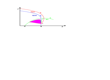
Figure 1: Schematic phase diagram of iron pnictides on the $x-T$ plane Moon2010PRB ; Fernandes2013PRL ; Fernandes2014NPhys , where $x$ denotes the doping concentration. The two points $x_{1}$ and $x_{2}$ are the SC and SDW QCPs, respectively. The nematic transition line bends back towards lower $x$ in the SC dome, showing reentrant behavior Nandi .

It is known Levchenko2013PRL ; Fernandes2013PRL that many of the physical properties of BaFe₂(As_1-xP_x)₂ and $\mathrm{Ba(Fe_{1-x}Co_{x})_{2}As_{2}}$ can be described by a three-band model that composed of one hole pocket located at the center of the Brillouin zone $\mathbf{Q}_{\Gamma}=(0,0)$ and two electron pockets centered at two specific momenta $\mathbf{Q}_{X}=(\pi,0)$ and $\mathbf{Q}_{Y}=(0,\pi)$. The Hamiltonian is usually written as Fernandes2013PRL

$$H=\sum_{\mathbf{k},i\in(X,Y,\Gamma)}\varepsilon_{\mathbf{k},i}c^{\dagger}_{\mathbf{k}\sigma,i}c_{\mathbf{k}\sigma,i}+H_{4},$$ (1)

where $H_{4}$ represents two sorts of interactions:

$$H_{4} = \sum_{\mathbf{k},i\in(X,Y)}\frac{U_{3}}{2}\left(c^{\dagger}_{\mathbf{k}\alpha,\Gamma}c^{\dagger}_{\mathbf{k}\gamma,\Gamma}c_{\mathbf{k}\delta,i}c_{\mathbf{k}\beta,i}+\mathrm{h.c.}\right)\delta_{\alpha\beta}\delta_{\gamma\delta}$$ (2)

$$+\sum_{\mathbf{k},i\in(X,Y)}U_{1}c^{\dagger}_{\mathbf{k}\alpha,\Gamma}c^{\dagger}_{\mathbf{k}\gamma,i}c_{\mathbf{k}\delta,i}c_{\mathbf{k}\beta,\Gamma}\delta_{\alpha\beta}\delta_{\gamma\delta}.$$

Here, $U_{3}$ denotes the pair hoping interaction and $U_{1}$ the density-density interaction, which are responsible for the SDW order and superconductivity respectively Fernandes2013PRL ; Maiti2010PRB . We mention here that the $U_{3}$ terms describe the magnetic Hund’s coupling interactions Chubukov2008PRB ; Lee2009PRL , which are known to be important in multi-band electronic systems Medici2011PRB ; Schickling2012PRL ; Medici2014PRL . As demonstrated in Ref. Fernandes2013PRL , the fermionic degrees of freedom can be fully integrated out, leading to

$$\mathcal{L} = \frac{1}{2}(\partial_{\mu}M_{X})^{2}+\frac{1}{2}(\partial_{\mu}M_{Y})^{2}+a_{m}(M^{2}_{X}+M^{2}_{Y})$$ (3)

$$+\frac{u_{m}}{2}(M^{2}_{X}+M^{2}_{Y})^{2}-\frac{g_{m}}{2}(M^{2}_{X}-M^{2}_{Y})^{2}$$

$$+\partial_{\mu}\Delta^{\dagger}\partial_{\mu}\Delta+a_{s}\Delta^{2}+\frac{u_{s}}{2}\Delta^{4}$$

$$+\zeta(M^{2}_{X}+M^{2}_{Y})\Delta^{2},$$

where the parameters $a_{m}$, $a_{s}$, $u_{s}$, $u_{m}$, $g_{m}$, and $\zeta$ are defined in Fernandes2013PRL . This model will be our starting point. The transition lines for the SDW and SC orders are obtained by taking $a_{m}=0$ and $a_{s}=0$, respectively. $M_{X,Y}$ represent the SDW order parameters that generate long-range magnetic order for $(\pi,0)$ and $(0,\pi)$ respectively Fernandes2012PRB ; Fernandes2013PRL . For $s^{+-}$-wave superconductor, a universal SC gap is introduced such that $\Delta_{\Gamma}=-\sqrt{2}\Delta_{X,Y}=\Delta$ Fernandes2013PRL . An Ising-type nematic order is induced by the magnetic order Fernandes2012PRB , and represented by the $M^{2}_{X}-M^{2}_{Y}$.

Fernandes et al. Fernandes2013PRL have recently studied the nature of quantum phase transitions in iron pnictides within the above effective theory and argued that the SDW and nematic orders merge at certain point in the SC dome. In this paper, we will make a systematic RG analysis. Our aim is two fold. First, we would like to examine the impact of the quantum fluctuations of SC and magnetic order parameters on the fate of phase transitions and the global phase diagram of the system, since these quantum fluctuations are known to play a vital role in systems that exhibit competing orders She2010PRB ; Millis2010 ; Wang2014PRD . Second, we attempt to extract the $T$-dependence of the superfluid density $\rho_{s}(T)$ from the RG solutions. As aforementioned, $\rho_{s}(T)$ can be suppressed by two different scenarios: the competitive interaction between distinct orders, and the coupling between fermionic quasiparticles and competing order. While the latter scenario has been studied in some recent references Levchenko2013PRL ; Ikeda2013PRL , the former is rarely considered in the literature Liu2012PRB . As will be shown below, the influence of ordering competition on $\rho_{s}(T)$ is prominent and can be efficiently obtained from our RG results.

To simplify consideration, we first concentrate on the SDW QCP, corresponding to $x_{2}$ on Fig. 1, at which $a_{m}=0$ and the magnetic order parameters have vanishing mean values, i.e., $\langle M_{X}\rangle=\langle M_{Y}\rangle=0$. In the SC dome, the SC order parameter develops a nonzero mean value, i.e., $\langle\Delta\rangle=V_{0}=\sqrt{-a_{s}/u_{s}}$. To study the quantum fluctuation of $\Delta$ around $\langle\Delta\rangle$, we introduce two new fields $h$ and $\eta$, and then decompose $\Delta$ as $\Delta=V_{0}+\frac{1}{\sqrt{2}}(h+i\eta)$ with $\langle h\rangle=\langle\eta\rangle=0$. Moreover, to compute the superfluid density, it is convenient to couple $\Delta$ to a gauge potential $A$. Recall that an important property of SC state is the happening of Anderson-Higgs mechanism, which leads to the Meissner effect. This mechanism needs to be properly included in the RG analysis. We now introduce gauge potential $A$ to the effective theory via the standard minimal coupling, i.e., $\partial_{\mu}\Delta\rightarrow(\partial_{\mu}-i\zeta_{\Delta A}A_{\mu})\Delta$, where $\zeta_{\Delta A}$ is the coupling between $A$ and $\Delta$. Straightforward calculations gives rise to the following effective model

$$\mathcal{L}_{\mathrm{eff}} = \frac{1}{2}(\partial_{\mu}M_{X})^{2}+\frac{1}{2}(\partial_{\mu}M_{Y})^{2}+\alpha_{X}M^{2}_{X}+\alpha_{Y}M^{2}_{Y}$$ (4)

$$+\frac{\beta_{X}}{2}M^{4}_{X}+\frac{\beta_{Y}}{2}M^{4}_{Y}+\zeta_{XY}M^{2}_{X}M^{2}_{Y}$$

$$+\frac{1}{2}(\partial_{\mu}h)^{2}+\alpha_{h}h^{2}+\frac{\beta_{h}}{2}h^{4}+\gamma_{h}h^{3}$$

$$-\frac{1}{4}\left(\partial_{\mu}A_{\nu}-\partial_{\nu}A_{\mu}\right)^{2}+\frac{\alpha_{A}}{2}A^{2}$$

$$+\gamma_{X^{2}h}M^{2}_{X}h+\gamma_{Y^{2}h}M^{2}_{Y}h+\zeta_{Xh}M^{2}_{X}h^{2}$$

$$+\zeta_{Yh}M^{2}_{Y}h^{2}+\gamma_{hA^{2}}hA^{2}+\zeta_{hA}h^{2}A^{2},$$

where we have defined a number of new effective parameters from $a_{m}$, $a_{s}$, $u_{s}$, $u_{m}$, $g_{m}$, $\zeta$, and $\zeta_{\Delta A}$:

$$\alpha_{X}=\alpha_{Y}\equiv a_{m}-\frac{a_{s}\zeta}{u_{s}},\beta_{X}=\beta_{Y}\equiv u_{m}-g_{m},$$

$$\alpha_{h}\equiv-a_{s},\beta_{h}\equiv\frac{u_{s}}{4},\gamma_{h}\equiv\sqrt{\frac{-a_{s}u_{s}}{2}},\alpha_{A}\equiv-\frac{2a_{s}\zeta_{\Delta A}}{u_{s}},$$

$$\gamma_{hA^{2}}\equiv\zeta_{\Delta A}\sqrt{\frac{-2a_{s}}{u_{s}}},\gamma_{X^{2}h}=\gamma_{Y^{2}h}\equiv\zeta\sqrt{\frac{-2a_{s}}{u_{s}}},$$

$$\zeta_{XY}\equiv(u_{m}+g_{m}),\zeta_{Xh}=\zeta_{Yh}\equiv\frac{\zeta}{2},\zeta_{hA}\equiv\frac{\zeta_{\Delta A}}{2},$$ (5)

As a consequence of the Anderson-Higgs mechanism, the massless Goldstone boson induced by gauge symmetry breaking is swallowed by the gauge boson $A$, which then acquires an effective mass term $\frac{1}{2}\alpha_{A}A^{2}$. The superfluid density $\rho_{s}$ is proportional to the gauge boson mass, i.e., $\rho_{s}\propto\alpha_{A}$ Halperin1974PRL . In the following, we will extract the $T$-dependence of $\rho_{s}(T)$ by computing the $l$-dependence of $\alpha_{A}\equiv\alpha_{A}(l)$, where $l$ is a running length scale. However, $\alpha_{A}$ is related intimately to other parameters, so we need to solve all the RG equations self-consistently.

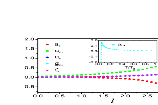
Figure 2: Flows of $a_{s}$, $u_{m}$, $u_{s}$, $g_{m}$ and $\zeta$ and $T$-dependence of $g_{m}$ (inset) at SDW QCP. The parameter $g_{m}$ is positive at small $l$ and high $T$, but becomes negative suddenly once $l$ exceeds some critical value $l_{m}$ and $T$ is lower than $T_{m}$.

As shown in Eq. (5), all the new effective parameters are given by the seven original parameters. Our RG calculations are performed to the one-loop level in powers of the coupling constants. Analogous to the analysis of Ref. Wang2014PRD , we have derived the RG equations for all the coupling parameters (See Supplemental Material Suppl for the details).

To solve the equations, we assign the initial values of parameters as $a_{s}=-0.001,u_{m}=0.05,u_{s}=0.01,g_{m}=0.01,\zeta=0.01$, and $\zeta_{\Delta A}=1.0\times 10^{-8}$. SC and SDW orders are supposed to coexist, so $u_{s}$, $u_{m}$, $g_{m}$, and $\zeta$ satisfy the constraint $\zeta<\sqrt{u_{s}(u_{m}-g_{m})}$ Schmalian2010PRB ; Fernandes2013PRL . The main conclusion is independent of these assumptions. There are three main results, to be explained one by one below.

First of all, we consider the fate of the associated phase transitions. After solving the RG equations, we show the $l$-dependence of various parameters in Fig. 2. The quadratic coupling parameters $u_{m}$, $u_{s}$, and $\zeta$ all flow to infinity eventually as $l\rightarrow+\infty$, thus the system does not approach any stable fixed point in the low energy region. As discussed in previous works She2010PRB ; Millis2010 ; Wang2014PRD ; Domany_Chen_Rudnick_Iacobson , this results is usually regarded as a signature of an instability towards first-order transitions since a second-order transition is always associated with the presence of a stable infrared fixed point Wilson1975RMP . However, we can see from Fig. 2 that the parameters $u_{m}$, $u_{s}$, and $\zeta$ increase with growing $l$ very slowly for small values of $l$. Their magnitudes become large only when $l$ grows beyond certain threshold. Therefore, before running to large values, the RG results of the $l$-dependence of these parameters are still reliable and give us very useful information about the physical properties of the system Wang2014PRB .

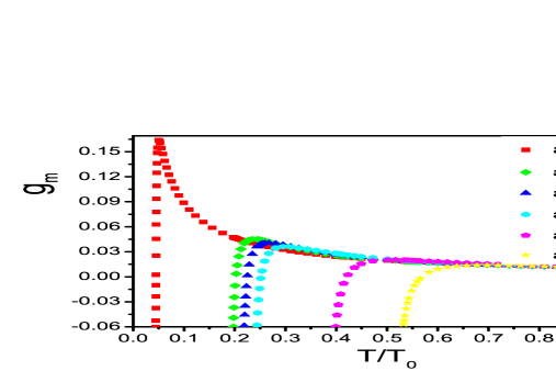
Figure 3: $T$-dependence of $g_{m}$ for different values of bare parameter $a^{0}_{m}$, which measures the distance to SDW QCP $x_{2}$. As $a_{m}^{0}$ grows, $g_{m}$ varies with $T$ similarly, but its peak disappears and the temperature for $g_{m}$ to change sign increases.

Secondly, we address the impact of the ordering competition on the nematic transition line. A number of experiments have observed an interesting transition from an orthorhombic structure to a tetragonal structure at low $T$ in the SC dome of $\mathrm{Ba(Fe_{1-x}Co_{x})_{2}As_{2}}$ Nandi ; Pratt2009PRL ; Christianson2009PRL and $\mathrm{Ba(Fe_{1-x}Rh_{x})_{2}As_{2}}$ Kreyssig2010PRB . It turns out that the nematic order exists in an intermediate range of $T$ and disappears once $T$ is lower than certain value. Remarkably, this unusual behavior can be naturally obtained in our RG analysis. To demonstrate this, let us consider the property of parameter $g_{m}$, whose sign determines whether the nematic order is present. If $g_{m}>0$, only one of the two order parameters $M_{X}$ and $M_{Y}$ develops a finite mean value Fernandes2012PRB ; Fernandes2014NPhys ; Fernandes1504.03656 due to tetragonal symmetry breaking. In this case, the nematic order is present. On the other hand, we have $\langle M_{X}\rangle=\langle M_{Y}\rangle$ if $g_{m}<0$, which indicates that the nematic order is absent Fernandes2012PRB ; Fernandes2014NPhys ; Fernandes1504.03656 . Therefore, to judge whether the nematic order exists at certain $T$, we need to compute the $T$-dependence of $g_{m}$ from the RG results.

The detailed $l$-dependence of $g_{m}$ is depicted in Fig. 2. As $l$ grows, $g_{m}$ first increases steadily, but decreases rapidly for large values of $l$ and becomes negative at certain critical value $l_{m}$. Notice that $l_{m}$ is also the length scale at which $u_{m}$, $u_{s}$, and $\zeta$ diverge. We can translate the $l$-dependence of $g_{m}$ to a $T$-dependence by using the transformation She2015PRB $T=T_{0}e^{-l}$. The inset of Fig. 2 clearly shows that the positive $g_{m}$ becomes negative as $T$ decreases immediately below temperature $T_{m}=T_{0}e^{-l_{m}}$, which means the nematic order is entirely suppressed at $T<T_{m}$. Therefore, the nematic order can only exist in the intermediate range between $T_{m}$ and its transition temperature $T_{n}$. It is destroyed by the thermal fluctuation at $T>T_{n}$, and by the strong competition among superconductivity, SDW, and nematic order at $T<T_{m}$. Since $T_{n}$ is supposed to be always higher than $T_{M}$ Fernandes2013PRL , this behavior gives rise to a back-bending effect of the nematic transition line on the phase diagram shown in Fig. 1, which is consistent with the observed reentrance of tetragonal structure at low temperatures Nandi .

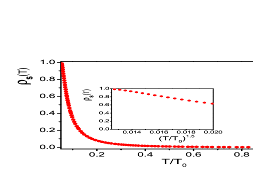
Figure 4: Strong $T$-dependence of superfluid density $\rho_{s}(T)$ at the SDW QCP. The inset shows that $\rho_{s}(T)$ is similar to $(T/T_{0})^{1.5}$ only in a very restricted temperature range.

To acquire a better knowledge of the phase diagram, we also wish to know how the nematic transition line varies with $T$ as we move away from the SDW QCP. In the doping region $x_{1}<x<x_{2}$, the SDW order parameters $M_{X}$ and $M_{Y}$ develop finite mean values. We here only present the main results (See Supplemental Material Suppl for more details). Fig. 3 shows the $T$-dependence of $g_{m}$ for different values of bare parameter $a_{m}^{0}$. For the chosen values of $a_{m}^{0}$, $g_{m}$ always first grows with decreasing $T$ and then becomes negative once $T$ is below certain threshold, which means the nematic order is suppressed at low $T$. In addition, the temperature scale at which $g_{m}$ changes sign increases as $a_{m}^{0}$ grows. In principle, the quantity $T_{0}$, given by the SC transition temperature, also varies as $a_{m}^{0}$ grows. However, despite this complexity, one can conclude from our RG results that the nematic transition line cannot intersect with the horizontal axis of Fig. 1, but should instead merge somewhere with the SC transition line. This property leads to a considerable modification of the global phase diagram, as visualized in Fig. 1. According to our results, the reentrance of tetragonal phase occur in a wide range of doping $x$.

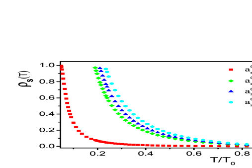
Figure 5: $\rho_{s}(T)$ at different values of $a_{m}^{0}$. The suppression of superfluid density takes place for any $a_{m}^{0}$, but is most significant at the SDW QCP where $a_{m}^{0}=0$.

Finally, we turn to the $T$-dependence of superfluid density $\rho_{s}$. Within the effective model given by Eq. (4), the superfluid density $\rho_{s}\propto\alpha_{A}=-\frac{2a_{s}\zeta_{\Delta A}}{u_{s}}$. To obtain the $T$-dependent $\lambda_{L}(T)$, we also utilize the transformation $T=T_{0}e^{-l}$, where a suitable choice of $T_{0}$ is the SC temperature $T_{c}$. At first glance, the RG results seem to suggest that $\rho_{s}\propto\lambda_{L}^{-2}$ diverges rapidly at $T_{m}$. However, because the transitions become first order, the $T$-dependence of $\rho_{s}(T)$ is reliable only at $T>T_{m}$. Here, we choose the value $\rho_{s}(T^{\ast})$ with $T^{\ast}$ being a little higher than $T_{m}$ to re-scale $\rho_{s}(T)$, and then show $\rho_{s}(T)/\rho(T^{\ast})$ in Fig. 4, where the initial values are the same as those adopted in Fig. 2. An obvious conclusion is that the ordering competition leads to a strong $T$-dependence of $\rho_{s}$, which decreases very rapidly as $T$ grows. For finite $a_{m}^{0}$, the behaviors of $\rho_{s}(T)$ are depicted in Fig. 5. As $a_{m}^{0}$ increases, the suppression of $\rho_{s}(T)$ becomes weaker. Since $T_{c}$ sensitively depends on the superfluid density, we can infer that $T_{c}$ should be suppressed to some extent in the region $x_{1}<x<x_{2}$ and that this effect is most significant at $x_{2}$, as shown in Fig. 1.

Hashimoto et al. Hashimoto2012PNAS has measured the superfluid density $\rho_{s}(T)$ in a number of superconductors, including iron pnictides and heavy fermion compounds, and claimed to unveil a universal $\rho_{s}(T)\propto T^{1.5}$ behavior over a wide range of temperatures. This behavior was argued Hashimoto2012PNAS ; Ikeda2013PRL to be caused by the coupling between magnetic fluctuation and fermionic excitations. Our analysis has clearly showed that ordering competition alone cannot account for the $\rho_{s}(T)\propto T^{1.5}$ behavior. As depicted in the inset of Fig. 4, only in a very restricted region of $T$ could we extract an approximate $(T/T_{0})^{1.5}$ behavior. On the other hand, we can see from the main panel of Fig. 4 that, ordering competition does make a significant contribution to $\rho_{s}(T)$ and hence cannot be simply neglected. Bearing these two points in mind, we believe that both ordering competition and fermionic excitations need to be properly incorporated in a more refined model of $\rho_{s}(T)$.

In summary, we have studied the impact of the strong competition among superconductivity, SDW order, and nematic order on the global phase diagram of iron pnictides by performing a systematic RG analysis within an effective field theory. The main results are summarized in the schematic phase diagram presented in Fig. 1.

J.W. is supported by the China Postdoctoral Science Foundation under Grants 2015T80655 and 2014M560510, the National Natural Science Foundation of China under Grant 11504360 and the Fundamental Research Funds for the Central Universities (P. R. China) under Grant WK2030040074. G.Z.L. is supported by the National Natural Science Foundation of China under Grant 11274286.

I Supplementary Material: Impact of ordering competition on the global phase diagram of iron pnictides

The 122-family iron-based superconductors, such as BaFe₂(As_1-xP_x)₂ and $\mathrm{Ba(Fe_{1-x}Co_{x})_{2}As_{2}}$ are widely described in the literature Levchenko2013PRL ; Fernandes2013PRL by a three-band model that is composed of one hole pocket located at the center of the Brillouin zone $\mathbf{Q}_{\Gamma}=(0,0)$ and two electron pockets centered at two specific momenta $\mathbf{Q}_{X}=(\pi,0)$ and $\mathbf{Q}_{Y}=(0,\pi)$. Recently, this model was used by Fernandes et al. to study the nature of quantum phase transitions in the superconducting dome of some iron pnictides Fernandes2013PRL . After integrating out the fermionic degrees of freedom Fernandes2013PRL and including the kinetic terms, one can obtain an effective Lagrangian density

$$\mathcal{L} = \frac{1}{2}(\partial_{\mu}M_{X})^{2}+\frac{1}{2}(\partial_{\mu}M_{Y})^{2}+a_{m}(M^{2}_{X}+M^{2}_{Y})+\frac{u_{m}}{2}(M^{2}_{X}+M^{2}_{Y})^{2}-\frac{g_{m}}{2}(M^{2}_{X}-M^{2}_{Y})^{2}$$ (6)

$$+\partial_{\mu}\Delta^{\dagger}\partial_{\mu}\Delta+a_{s}\Delta^{2}+\frac{u_{s}}{2}\Delta^{4}+\zeta(M^{2}_{X}+M^{2}_{Y})\Delta^{2},$$

where the parameters $a_{m}$, $a_{s}$, $u_{s}$, $u_{m}$, $g_{m}$, and $\zeta$, are defined in Ref. Fernandes2013PRL . Our RG analysis starts from this effective field theory. In order to examine the effect of ordering competition on the superfluid density, we introduce a small external gauge potential $A$ that couples to the superconducting order parameter Halperin1974PRL and thus have an additional term

$$\mathcal{L^{\prime}} = -\frac{1}{4}\left(\partial_{\mu}A_{\nu}-\partial_{\nu}A_{\mu}\right)^{2}+\zeta_{\Delta A}|\Delta|^{2}A^{2},$$ (7)

where the Lorentz gauge $\partial_{\mu}A_{\mu}=0$ is utilized and the parameter $\zeta_{\Delta A}$ is a new coupling constant.

In the superconducting dome, the order parameter $\Delta$ acquires a finite vacuum expectation value, i.e.,

$$V_{0}\equiv\langle\Delta\rangle=\sqrt{\frac{-a_{s}}{u_{s}}}.$$ (8)

The quantum fluctuation of $\Delta$ around its mean value is believed to play an important role Wang2014PRD and needs to be seriously taken into account. It is convenient to introduce two new fields $h$ and $\eta$ by defining

$$\Delta=V_{0}+\frac{1}{\sqrt{2}}(h+i\eta),$$ (9)

with $\langle h\rangle=\langle\eta\rangle=0$. In many field-theoretic treatments of ordering competition, specially in the context of condensed matter systems, the quantum fluctuation of order parameter in the ordered phase is usually omitted. However, more careful analysis Wang2014PRD have showed that this approximation is not appropriate and that the order parameter fluctuation around its mean value can be significant. In order to entirely reveal the physical effects of ordering competition, we will consider $h$ and $\eta$ as quantum field operators and study their interactions with the magnetic order parameters $M_{X}$ and $M_{Y}$.

Substituting the re-parameterized field operator Eq. (9) into the total Lagrangian density, we get a new effective model

$$\mathcal{L}_{\mathrm{eff}} = \frac{1}{2}(\partial_{\mu}M_{X})^{2}+\frac{1}{2}(\partial_{\mu}M_{Y})^{2}+\alpha_{X}M^{2}_{X}+\alpha_{Y}M^{2}_{Y}+\frac{\beta_{X}}{2}M^{4}_{X}+\frac{\beta_{Y}}{2}M^{4}_{Y}+\zeta_{XY}M^{2}_{X}M^{2}_{Y}$$ (10)

$$+\frac{1}{2}(\partial_{\mu}h)^{2}+\alpha_{h}h^{2}+\frac{\beta_{h}}{2}h^{4}+\gamma_{h}h^{3}-\frac{1}{4}\left(\partial_{\mu}A_{\nu}-\partial_{\nu}A_{\mu}\right)^{2}+\frac{\alpha_{A}}{2}A^{2}+\gamma_{X^{2}h}M^{2}_{X}h$$

$$+\gamma_{Y^{2}h}M^{2}_{Y}h+\zeta_{Xh}M^{2}_{X}h^{2}+\zeta_{Yh}M^{2}_{Y}h^{2}+\gamma_{hA^{2}}hA^{2}+\zeta_{hA}h^{2}A^{2},$$

where a number of effective parameters are defined on the basis of the fundamental parameters $a_{m}$, $a_{s}$, $u_{s}$, $u_{m}$, $g_{m}$, $\zeta$, and $\zeta_{\Delta A}$, as given by Eq. (5) in the main part of the paper. Our RG analysis will be based on this effective model, assuming that the coupling constants take small values.

We now proceed to treat the effective theory by performing a detailed RG analysis Shankar1994RMP . To this end, we first make the following scaling transformations

$$k_{i} = k^{\prime}_{i}e^{-l},$$

$$\omega = \omega^{\prime}e^{-l},$$

$$q_{i} = q^{\prime}_{i}e^{-l},$$

$$\epsilon = \epsilon^{\prime}e^{-l},$$ (11)

where $i=x,y$ and $l$ is a running length scale. Under these transformations, the field operators $M_{X}$, $M_{Y}$, $h$, and $\eta$ should be re-scaled as

$$M_{X}(\mathbf{k},\omega) = M^{\prime}_{X}(\mathbf{k^{\prime}},\omega^{\prime})e^{5l/2},$$

$$M_{Y}(\mathbf{k},\omega) = M^{\prime}_{Y}(\mathbf{k^{\prime}},\omega^{\prime})e^{5l/2},$$

$$h(\mathbf{k},\omega) = h^{\prime}(\mathbf{k^{\prime}},\omega^{\prime})e^{5l/2},$$

$$A(\mathbf{q},\epsilon) = A^{\prime}(\mathbf{q^{\prime}},\epsilon^{\prime})e^{5l/2}.$$ (12)

In order to obtain the flow equations of the fundamental parameters defined in Eq. (6) and Eq. (7), we apply the following identifies:

$$\frac{da_{s}}{dl} = -\frac{d\alpha_{h}}{dl},$$

$$\frac{du_{s}}{dl} = 4\frac{d\beta_{h}}{dl},$$

$$\frac{da_{m}}{dl} = \frac{d\alpha_{X}}{dl}+\frac{\zeta}{u_{s}}\frac{da_{s}}{dl}+\frac{a_{s}}{u_{s}}\frac{d\zeta}{dl}-\frac{a_{s}\zeta}{u_{s}^{2}}\frac{du_{s}}{dl},$$

$$\frac{du_{m}}{dl} = \frac{1}{2}\frac{d\zeta_{XY}}{dl}+\frac{1}{2}\frac{d\beta_{X}}{dl},$$

$$\frac{dg_{m}}{dl} = \frac{1}{2}\frac{d\zeta_{XY}}{dl}-\frac{1}{2}\frac{d\beta_{X}}{dl},$$

$$\frac{d\zeta}{dl} = 2\frac{d\zeta_{Xh}}{dl},$$

$$\frac{d\zeta_{\Delta A}}{dl} = 2\frac{d\zeta_{hA}}{dl}.$$ (13)

For simplicity, we first consider the SDW QCP with $a_{m}=0$, where the magnetic order parameters $M_{X}$ and $M_{Y}$ both have vanishing mean values and their quantum fluctuations are critical. Analogous to the scheme presented in Ref. Wang2014PRD , we have derived the following RG equations for the seven fundamental parameters

$$\left.\begin{array}[]{ll}\frac{da_{s}}{dl}=2a_{s}-\frac{1}{12\pi^{2}}\left[\frac{27a_{s}u_{s}}{2}(1+4a_{s})+\frac{12a_{s}\lambda^{2}}{u_{s}}\left(1+\frac{4a_{s}\lambda}{u_{s}}\right)+3\lambda\left(1+\frac{2a_{s}\lambda}{u_{s}}\right)\right.\\ \hskip 21.90874pt\left.+\frac{9u_{s}}{4}(1+2a_{s})+3\lambda_{\Delta A}\left(1+\frac{2a_{s}\lambda_{\Delta A}}{u_{s}}\right)+\frac{32a_{s}\lambda^{2}_{\Delta A}}{u_{s}}\left(1+\frac{4a_{s}\lambda_{\Delta A}}{u_{s}}\right)\right].\\ \frac{du_{m}}{dl}=u_{m}+\frac{1}{2\pi^{2}}\left\{(8u_{m}g_{m}-17u^{2}_{m}-11g^{2}_{m})\left(\frac{4a_{s}\lambda}{u_{s}}+1\right)-\frac{3\lambda^{2}}{8}(4a_{s}+1)\right.\\ \hskip 21.90874pt\left.+\frac{16a_{s}\lambda^{2}}{u_{s}}(2u_{m}-g_{m})\left(1+\frac{4a_{s}\lambda}{u_{s}}+2a_{s}\right)-\frac{6a_{s}\lambda^{3}}{u_{s}}\left[1+2\left(\frac{a_{s}\lambda}{u_{s}}+2a_{s}\right)\right]\right\},\\ \frac{du_{s}}{dl}=u_{s}+\frac{1}{\pi^{2}}\left\{2\lambda^{2}\left[4\left(a_{m}-\frac{a_{s}\lambda}{u_{s}}\right)-1\right]-\frac{9u^{2}_{s}}{4}(4a_{s}+1)+54a_{s}u^{2}_{s}(1+6a_{s})\right.\\ \hskip 21.90874pt\left.-\frac{4\lambda^{2}_{\Delta A}}{3}\left(\frac{4a_{s}\lambda_{\Delta A}}{u_{s}}+1\right)+\frac{32a_{s}\lambda^{3}}{u_{s}}\left(1+\frac{6a_{s}\lambda}{u_{s}}\right)+\frac{11072a_{s}\lambda^{3}_{\Delta A}}{35u_{s}}\left(1+\frac{6a_{s}\lambda_{\Delta A}}{u_{s}}\right)\right\},\\ \frac{dg_{m}}{dl}=g_{m}+\frac{1}{2\pi^{2}}\left\{3(u_{m}^{2}+3g^{2}_{m}-8u_{m}g_{m})\left(\frac{4a_{s}\lambda}{u_{s}}+1\right)+\frac{\lambda^{2}}{8}(4a_{s}+1)\right.\\ \hskip 21.90874pt\left.+\frac{16a_{s}\lambda^{2}}{u_{s}}(2g_{m}-u_{m})\left(1+\frac{4a_{s}\lambda}{u_{s}}+2a_{s}\right)-\frac{2a_{s}\lambda^{3}}{u_{s}}\left[1+2\left(\frac{a_{s}\lambda}{u_{s}}+2a_{s}\right)\right]\right\},\\ \frac{d\lambda}{dl}=\lambda+\frac{1}{\pi^{2}}\left[\frac{4a_{s}\lambda^{3}}{u_{s}}\left(1+\frac{4a_{s}\lambda}{u_{s}}+2a_{s}\right)-\frac{3u_{s}\lambda}{8}(4a_{s}+1)+9a_{s}u_{s}\lambda(1+6a_{s})-2\lambda^{2}\left(\frac{2a_{s}\lambda}{u_{s}}+2a_{s}+1\right)\right.\\ \hskip 21.90874pt\left.-\lambda(2u_{m}-g_{m})\left(\frac{4a_{s}\lambda}{u_{s}}+1\right)+\frac{16a_{s}\lambda^{2}}{u_{s}}(2u_{m}-g_{m})\left(1+\frac{6a_{s}\lambda}{u_{s}}\right)+6a_{s}\lambda^{2}\left(1+\frac{2a_{s}\lambda}{u_{s}}+4\alpha_{s}\right)\right],\\ \frac{d\lambda_{\Delta A}}{dl}=\lambda_{\Delta A}+\frac{1}{3\pi^{2}}\left\{27a_{s}u_{s}\lambda_{\Delta A}(1+6a_{s})-12\lambda^{2}_{\Delta A}\left(1+2a_{s}+\frac{2a_{s}\lambda_{\Delta A}}{u_{s}}\right)-\frac{9u_{s}\lambda_{\Delta A}}{8}(4a_{s}+1)\right.\\ \hskip 21.90874pt\left.+\frac{64a_{s}\lambda^{3}_{\Delta A}}{u_{s}}\left(1+2a_{s}+\frac{4a_{s}\lambda_{\Delta A}}{u_{s}}\right)+36a_{s}\lambda^{2}_{\Delta A}\left[1+2a_{s}\left(2+\frac{\lambda_{\Delta A}}{u_{s}}\right)\right]\right\}.\end{array}\right.$$ (26)

When the system moves away from the SDW QCP and goes to a lower doping concentration, the stripe-SDW order parameters $M_{X}$ and $M_{Y}$ also develop nonzero mean values, i.e.,

$$\langle M_{X}\rangle=\langle M_{Y}\rangle=\sqrt{-\frac{a_{m}}{2u_{m}}}.$$ (27)

To include the quantum fluctuation of $M_{X}$ and $M_{Y}$ around their mean values, we introduce two new fields $\xi$ and $\chi$:

$$M_{X} = \sqrt{-\frac{a_{m}}{2u_{m}}}+\xi,$$ (28)

$$M_{Y} = \sqrt{-\frac{a_{m}}{2u_{m}}}+\chi,$$ (29)

with $\langle\xi\rangle=\langle\chi\rangle=0$. Now the problem becomes more complicated than the case of SDW QCP. After lengthy but straightforward calculations, we obtain a set of RG equations:

$$\left.\begin{array}[]{ll}\frac{da_{s}}{dl}=2a_{s}-\frac{1}{4\pi^{2}}\Bigl{\{}\frac{18a_{s}u_{s}}{4}(1+4a_{s})+\frac{4a_{s}\lambda^{2}}{u_{s}}\Bigl{[}1+4\Bigl{(}\frac{a_{s}\lambda}{u_{s}}+a_{m}\Bigr{)}\Bigr{]}+\frac{32a_{s}\lambda^{2}_{\Delta A}}{3u_{s}}\Bigl{(}1+\frac{4\lambda_{\Delta A}a_{s}}{u_{s}}\Bigr{)}+\lambda\Bigl{[}1+2\Bigl{(}\frac{a_{s}\lambda}{u_{s}}+a_{m}\Bigr{)}\Bigr{]}\\ \hskip 21.90874pt+\frac{3u_{s}}{4}(1+2a_{s})+\frac{8a_{s}a^{2}_{m}\lambda^{2}}{u_{s}}\Bigl{[}1+8\Bigl{(}\frac{a_{s}\lambda}{u_{s}}+a_{m}\Bigr{)}\Bigr{]}+\lambda_{\Delta A}\Bigl{(}1+\frac{2\lambda_{\Delta A}a_{s}}{u_{s}}\Bigr{)}+4a^{2}_{m}\lambda\Bigl{[}1+6\Bigl{(}\frac{a_{s}\lambda}{u_{s}}+a_{m}\Bigr{)}\Bigr{]}\Bigr{\}},\\ \frac{da_{m}}{dl}=2\Bigl{(}\frac{a_{s}\lambda}{u_{s}}+a_{m}\Bigr{)}+\frac{1}{4\pi^{2}}\Bigl{\{}12a_{m}\Bigl{[}a_{m}(g_{m}+5u_{m})-6u_{m}\Bigr{]}\Bigl{[}1+4\Bigl{(}\frac{a_{s}\lambda}{u_{s}}+a_{m}\Bigr{)}\Bigr{]}-72a^{3}_{m}u_{m}\Bigl{[}1+8\Bigl{(}\frac{a_{s}\lambda}{u_{s}}+a_{m}\Bigr{)}\Bigr{]}\\ \hskip 21.90874pt-\frac{4a_{s}\lambda^{2}}{u_{s}}\Bigl{[}1+2\Bigl{(}\frac{a_{s}\lambda}{u_{s}}+a_{m}\Bigr{)}+2a_{s}\Bigr{]}-2(2u_{m}-g_{m})\Bigl{[}1+2\Bigl{(}\frac{a_{s}\lambda}{u_{s}}+a_{m}\Bigr{)}\Bigr{]}-\frac{\lambda}{2}(1+2a_{s})\\ \hskip 21.90874pt-4a^{2}_{m}(g_{m}-17u_{m})\Bigl{[}1+6\Bigl{(}\frac{a_{s}\lambda}{u_{s}}+a_{m}\Bigr{)}\Bigr{]}\Bigr{\}}+\left(\frac{\lambda}{u_{s}}\frac{da_{s}}{dl}+\frac{a_{s}}{u_{s}}\frac{d\lambda}{dl}-\frac{a_{s}\lambda}{u_{s}^{2}}\frac{du_{s}}{dl}\right),\\ \frac{du_{m}}{dl}=u_{m}+\frac{1}{4\pi^{2}}\Bigl{\{}576a_{m}u_{m}(2u_{m}-g_{m})\left[1+6\Bigl{(}\frac{a_{s}\lambda}{u_{s}}+a_{m}\Bigr{)}\Bigr{]}-16a^{2}_{m}\Bigl{(}130u^{2}_{m}-94u_{m}g_{m}+g^{2}_{m}\Bigr{)}\Bigl{[}1+8\Bigl{(}\frac{a_{s}\lambda}{u_{s}}+a_{m}\Bigr{)}\Bigr{]}\right.\\ \hskip 21.90874pt+\frac{32a_{s}\lambda^{2}}{u_{s}}(2u_{m}-g_{m})\Bigl{[}(1+4a^{2}_{m})(1+2a_{s})+4\Bigl{(}\frac{a_{s}\lambda}{u_{s}}+a_{m}\Bigr{)}(1+8a^{2}_{m})\Bigr{]}+\frac{16a_{s}\lambda^{3}}{u_{s}}\left[1+2\left(\frac{a_{s}\lambda}{u_{s}}+2a_{s}\right)\right]\\ \hskip 21.90874pt\left.-(37u^{2}_{m}+25g^{2}_{m}-10u_{m}g_{m})\Bigl{[}1+4\Bigl{(}\frac{a_{s}\lambda}{u_{s}}+a_{m}\Bigr{)}\Bigr{]}+4608a^{3}_{m}u_{m}(2u_{m}-g_{m})\Bigl{[}1+10\Bigl{(}\frac{a_{s}\lambda}{u_{s}}+a_{m}\Bigr{)}\Bigr{]}\right\},\\ \frac{dg_{m}}{dl}=g_{m}+\frac{1}{2\pi^{2}}\Bigl{\{}\frac{32a_{s}\lambda^{2}}{u_{s}}(2g_{m}-u_{m})\Bigl{[}(1+4a^{2}_{m})(1+2a_{s})+4\Bigl{(}\frac{a_{s}\lambda}{u_{s}}+a_{m}\Bigr{)}(1+8a^{2}_{m})\Bigr{]}\\ \hskip 21.90874pt-4a^{2}_{m}\Bigl{[}(g_{m}+73u_{m})(7g_{m}-5u_{m})+9(u_{m}-g_{m})^{2}\Bigr{]}\Bigl{[}1+8\Bigl{(}\frac{a_{s}\lambda}{u_{s}}+a_{m}\Bigr{)}\Bigr{]}\\ \hskip 21.90874pt-\Bigl{[}12(u_{m}-g_{m})(2g_{m}-u_{m})+6(u_{m}+g_{m})^{2}-\frac{\lambda^{2}}{4}\Bigr{]}\Bigl{[}4\Bigl{(}\frac{a_{s}\lambda}{u_{s}}+a_{m}\Bigr{)}+1\Bigr{]}\\ \hskip 21.90874pt+576a_{m}u_{m}(2g_{m}-u_{m})\Bigl{[}6\Bigl{(}\frac{a_{s}\lambda}{u_{s}}+a_{m}\Bigr{)}+1\Bigr{]}\Bigr{\}},\\ \frac{du_{s}}{dl}=u_{s}+\frac{4}{\pi^{2}}\left\{\frac{27a_{s}u^{2}_{s}}{2}(1+6a_{s})-\frac{144a_{s}a_{m}u_{m}\lambda^{3}}{u_{s}}\Bigl{[}1+10\Bigl{(}\frac{a_{s}\lambda}{u_{s}}+a_{m}\Bigr{)}\Bigr{]}-\frac{\lambda^{2}}{2}\Bigl{[}4\Bigl{(}\frac{a_{s}\lambda}{u_{s}}+a_{m}\Bigr{)}+1\Bigr{]}\right.\\ \hskip 21.90874pt-\frac{9u^{2}_{s}}{16}(4a_{s}+1)-\frac{4\lambda^{2}_{\Delta A}}{3}\Bigl{(}\frac{4\lambda_{\Delta A}a_{s}}{u_{s}}+1\Bigr{)}-a^{2}_{m}\lambda^{2}\Bigl{[}1+8\Bigl{(}\frac{a_{s}\lambda}{u_{s}}+a_{m}\Bigr{)}\Bigr{]}\\ \hskip 21.90874pt\left.+\frac{8a_{s}\lambda^{3}}{u_{s}}\left(1+\frac{6a_{s}\lambda}{u_{s}}\right)+\frac{2768a_{s}\lambda^{3}_{\Delta A}}{35u_{s}}\left(1+\frac{6a_{s}\lambda_{\Delta A}}{u_{s}}\right)\right\},\\ \frac{d\lambda}{dl}=\lambda+\frac{\lambda}{\pi^{2}}\left\{9a_{s}u_{s}(6a_{s}+1)+72a_{m}u_{m}\Bigl{[}6\Bigl{(}\frac{a_{s}\lambda}{u_{s}}+a_{m}\Bigr{)}+1\Bigr{]}-(2u_{m}-g_{m})\Bigl{[}4\Bigl{(}\frac{a_{s}\lambda}{u_{s}}+a_{m}\Bigr{)}+1\Bigr{]}\right.\\ \hskip 21.90874pt-\frac{3u_{s}}{8}(4a_{s}+1)+\frac{96a_{s}a^{2}_{m}\lambda^{2}}{u_{s}}\Bigl{(}\frac{a_{s}\lambda}{u_{s}}+a_{m}\Bigr{)}-2\lambda\Bigl{[}1-\frac{2a_{s}\lambda}{u_{s}}(1+4a^{2}_{m})\Bigr{]}\Bigl{[}2a_{s}+2\Bigl{(}\frac{a_{s}\lambda}{u_{s}}+a_{m}\Bigr{)}+1\Bigr{]}\\ \hskip 21.90874pt-4a^{2}_{m}(20u_{m}-g_{m})\Bigl{[}1+8\Bigl{(}\frac{a_{s}\lambda}{u_{s}}+a_{m}\Bigr{)}\Bigr{]}+576a^{3}_{m}u_{m}\Bigl{(}1+10\Bigl{(}\frac{a_{s}\lambda}{u_{s}}+a_{m}\Bigr{)}\Bigr{)}\\ \hskip 21.90874pt\left.+\frac{16a_{s}\lambda}{u_{s}}(2u_{m}-g_{m})\left(1+\frac{6a_{s}\lambda}{u_{s}}\right)+6a_{s}\lambda\left[1+2a_{s}\left(\frac{\lambda}{u_{s}}+2\right)\right]\right\},\\ \frac{d\lambda_{\Delta A}}{dl}=\lambda_{\Delta A}+\frac{\lambda_{\Delta A}}{3\pi^{2}}\left\{27a_{s}u_{s}(1+6a_{s})-\frac{9u_{s}}{8}(4a_{s}+1)+\frac{64a_{s}\lambda^{2}_{\Delta A}}{u_{s}}\Bigl{[}1+2a_{s}\Bigl{(}1+\frac{2\lambda_{\Delta A}}{u_{s}}\Bigr{)}\Bigr{]}\right.\\ \hskip 21.90874pt\left.-12\lambda_{\Delta A}\Bigl{[}1+2a_{s}\Bigl{(}1+\frac{\lambda_{\Delta A}}{u_{s}}\Bigr{)}\Bigr{]}+36a_{s}\lambda_{\Delta A}\left[1+2a_{s}\left(2+\frac{\lambda_{\Delta A}}{u_{s}}\right)\right]\right\}.\end{array}\right.$$ (51)

These equations are used to analyze the impact of ordering competition on the global phase diagram in the main context of the paper.

References

(1)
P. A. Lee, N. Nagaosa, and X.-G. Wen, Rev. Mod. Phys. 78, 17
(2006).
(2)
H. v. Löhneysen, A. Rosch, M. Vojta, and P. Wölfle, Rev.
Mod. Phys. 79, 1015 (2007).
(3)
O. Stockert, S. Kirchner, F. Steglich, and Q. Si, J. Phys. Soc. Jpn.
81, 011001 (2012).
(4)
Y. Kamihara, T. Watanabe, M. Hirano, H. Hosono, J. Am. Chem. Soc.
130, 3296 (2008).
(5)
X. H. Chen, T. Wu, G. Wu, R. H. Liu, H. Chen, and D. F. Fang, Nature
(London) 453, 761 (2008).
(6)
G. F. Chen, Z. Li, D. Wu, G. Li, W. Z. Hu, J. Dong, P. Zheng,
J. L. Luo, and N. L. Wang, Phys. Rev. Lett. 100, 247002 (2008).
(7)
M. Rotter, M. Tegel, and D. Johrendt, Phys. Rev. Lett. 101,
107006 (2008).
(8)
I. R. Fisher, L. Degiorgi, and Z. X. Shen, Rep. Prog. Phys. 74, 124506 (2011).
(9)
P. J. Hirschfeld, M. M. Korshunov, and I. I. Mazin, Rep. Prog. Phys.
74, 124508 (2011).
(10)
A. V. Chubukov, Annu. Rev. Condens. Matter Phys. 3, 57 (2012).
(11)
M. Vojta, Adv. Phys. 58, 699 (2009); E. Fradkin et al.,
Annu. Rev. Condens. Matter Phys. 1, 153 (2010).
(12)
G.-Z. Liu, J.-R. Wang, and J. Wang, Phys. Rev. B 85, 174525
(2012).
(13)
K. Hashimoto, K. Cho, T. Shibauchi, S. Kasahara, Y. Mizukami, R.
Katsumata, Y. Tsuruhara, T. Terashima, H. Ikeda, M.A. Tanatar, H.
Kitano, N. Salovich, R.W. Giannetta, P.Walmsley, A. Carrington, R.
Prozorov, and Y. Matsuda, Science 336, 1554 (2012).
(14)
A. Levchenko, M. G. Vavilov, M. Khodas, and A.V. Chubukov, Phys.
Rev. Lett. 111, 177003 (2013).
(15)
D. Chowdhury, B. Swingle, E. Berg, and S. Sachdev, Phys. Rev. Lett.
111, 157004 (2013).
(16)
R. M. Fernandes, S. Maiti, P. Wölfle, and A. V. Chubukov,
Phys. Rev. Lett. 111, 057001 (2013).
(17)
K. G. Wilson, Rev. Mod. Phys. 47, 773 (1975).
(18)
R. Shankar, Rev. Mod. Phys. 66, 129 (1994).
(19)
E. G. Moon and S. Sachdev, Phys. Rev. B 82, 104516 (2010).
(20)
R. M. Fernandes, A. V. Chubukov, and J. Schmalian, Nat. Phys. 10, 97 (2014).
(21)
S. Nandi, M. G. Kim, A. Kreyssig, R. M. Fernandes, D. K. Pratt, A.
Thaler, N. Ni, S. L. Bud’ko, P. C. Canfield, J. Schmalian, R. J.
McQueeney, and A. I. Goldman, Phys. Rev. Lett. 104, 057006
(2010).
(22)
S. Maiti and A. V. Chubukov, Phys. Rev. B 82, 214515 (2010).
(23)
A. V. Chubukov, D. V. Efremov, and I. Eremin, Phys. Rev. B 78,
134512 (2008)
(24)
F. Wang, H. Zhai, Y. Ran, A. Vishwanath, D.-H. Lee
Phys. Rev. Lett. 102, 047005 (2009).
(25)
L. de’ Medici, Phys. Rev. B 83, 205112 (2011).
(26)
T. Schickling, F. Gebhard, J. Bünemannand, L. Boeri, O. K.
Andersen, and W. Webe, Phys. Rev. Lett. 108, 036406 (2012).
(27)
L. de’ Medici, G. Giovannetti, and M. Capone, Phys. Rev. Lett. 112, 177001 (2014).
(28)
R. M. Fernandes, A. V. Chubukov, J. Knolle, I. Eremin, and J.
Schmalian, Phys. Rev. B 85, 024534 (2012).
(29)
J.-H. She, J. Zaanen, A. R. Bishop, and A. V. Balatsky, Phys. Rev. B
82, 165128 (2010).
(30)
Z. Nussinov, I. Vekhter and A. V. Balatsky, Phys. Rev. B 79,
165122 (2009); A. J. Millis, Phys. Rev. B 81, 035117 (2010).
(31)
J. Wang and G.-Z. Liu, Phys. Rev. D 90, 125015 (2014).
(32)
T. Nomoto and H. Ikeda, Phys. Rev. Lett. 111, 167001 (2013).
(33)
See Supplemental Material at http:…. for more detailed analytical
treatment of the effective theory and for the expression of the
coupled RG equations of all the effective parameters.
(34)
B. I. Halperin, T. C. Lubensky, and S.-K. Ma, Phys. Rev. Lett. 32, 292 (1974).
(35)
R. M. Fernandes and J. Schmalian, Phys. Rev. B 82, 014521 (2010).
(36)
E. Domany, D. Mukamel, and M. E. Fisher, Phys. Rev. B 15, 5432
(1977); J. H. Chen, T. C. Lubensky, and D. R. Nelson, Phys. Rev. B
17, 4274 (1978); J. Rudnick, Phys. Rev. B 18, 1406
(1978); H. H. Iacobson and D. J. Amit, Ann. Phys. 133, 57
(1981).
(37)
J. Wang, A. Eberlein, and W. Metzner, Phys. Rev. B 89,
121116(R) (2014).
(38)
D. K. Pratt, W. Tian, A. Kreyssig, J. L. Zarestky, S. Nandi, N. Ni,
S. L. Bud’ko, P. C. Canfield, A. I. Goldman, and R. J. McQueeney,
Phys. Rev. Lett. 103, 087001 (2009).
(39)
A. D. Christianson, M. D. Lumsden, S. E. Nagler, G. J. Mac-Dougall,
M. A. McGuire, A. S. Sefat, R. Jin, B. C. Sales, and D. Mandrus,
Phys. Rev. Lett. 103, 087002 (2009).
(40)
A. Kreyssig, M. G. Kim, S. Nandi, D. K. Pratt, W. Tian, J. L.
Zarestky, N. Ni, A. Thaler, S. L. Bud’ko, P. C. Canfield, R. J.
McQueeney, and A. I. Goldman, Phys. Rev. B 81, 134512 (2010).
(41)
R. M. Fernandes, S. A. Kivelson, and E. Berg, arXiv:1504.03656.
(42)
J.-H. She, M. J. Lawler, and E.-A. Kim, Phys. Rev. B 92, 035112 (2015).
(43)
K. Hashimoto, Y. Mizukami, R. Katsumata, H. Shishido, M. Yamashita,
H. Ikeda, Y. Matsuda, J. A. Schlueter, J. D. Fletcher, A.
Carrington, D. Gnida, D. Kaczorowski, and T. Shibauchi, PNAS 110, 3293 (2013).