Embarrassingly Parallel Time Series Analysis for
Large Scale Weak Memory Systems

Abstract

Second order stationary models in time series analysis are based on the analysis of essential statistics whose computations follow a common pattern. In particular, with a map-reduce nomenclature, most of these operations can be modeled as mapping a kernel that only depends on short windows of consecutive data and reducing the results produced by each computation. This computational pattern stems from the ergodicity of the model under consideration and is often referred to as weak or short memory when it comes to data indexed with respect to time. In the following we will show how studying weak memory systems can be done in a scalable manner thanks to a framework relying on specifically designed overlapping distributed data structures that enable fragmentation and replication of the data across many machines as well as parallelism in computations. This scheme has been implemented for Apache Spark but is certainly not system specific. Indeed we prove it is also adapted to leveraging high bandwidth fragmented memory blocks on GPUs.

Introduction

Classic time series analysis and in particular that of second order stationary processes has been widely studied for several decades and reached a peak of popularity in the years 1980-1990 when computational power became more common and allowed for practical implementation of varied data sets. Monographs such as [1], [2] and [3] offered the opportunity for many researchers to better understand the intricacies of time series analysis. The topics of univariate and monovariate time series analysis were also well covered in [4, 5] and many other publications. Software such as R or Matlab has given the opportunity to many practitioners to examine data, enabling even more applications of time series analysis and contributing to the interest in that field. The amount of research dedicated to time series analysis has been so important in the past decades that we do not claim here to review it holistically. However, it is necessary to contextualize the topic of the present article both in its theoretical aspects and its practical implementation.
The development of distributed programming paradigms [6], file systems [7], databases [8] and in-memory computing engines [9] for the modern commodity datacenter environment has led us to consider new applications and implementations for time series analysis. As opposed to small dataset applications such as those developed in quantitative finance [10], climate studies [11], network traffic analysis [12], hydrology [13], we are now interested in analyzing observations at scale in a data intensive environment such as [14] with a standardized distributed library similar to MLlib [15]. This creates new challenges. In particular, we are dealing with data sitting on a distributed cluster of machines whose memory layout has an obvious bandwidth bottleneck when it comes to shuffling data across an Ethernet network. This also creates new opportunities. Time series estimation can now leverage recent theoretical developments [16] as well as improvements in convex optimization techniques [17, 18] that can help get likelihood maximization based estimators faster.
In this new programming framework, we will start adapting the implementation of the simplest class of models: linear time series models. These are the stochastic counterparts of deterministic linear systems [19]. Estimating auto-regressive and moving average models (weak memory models) will be the main focus of this document. More advanced topics such as the identification of non linear dynamics [20, 21] as well heteroscedastic systems [22] will be the subject of subsequent work.
This document focuses on the presentation of a new data structure dedicated to the representation of estimation-ready data sets for time series analysis. As opposed to other frameworks such as SparkTS, spark-timeseries or Thunder, the data is partitioned here with respect to time. An overlapping block distributed data structure has been devised which, given an appropriate padding expressed in units of time, enables the computation of M and Z estimators for second order stationary models in an embarrassingly parallel manner. This enables in particular the calibration of multivariate time series models without shuffling observations on a distributed in-memory computing engine.

Part I Theoretical background on time series analysis, estimators, motivation

Our intent is to provide a generic programming framework for scalable time series analysis in a distributed system. In the following, we review popular time series models that should be supported by the framework and establish the corresponding computational operations the related estimators require. Focus is set on second order stationary models and the the well known ARMA family.

1 Second order stationary time series

We start with the most common time series models. These are models in which observation are regularly spaced and for which there are no missing values. Practitioners of time series analysis are familiar with missing data, outliers and irregularly spaced timestamps. In such cases, an interpolation technique (linear interpolation or last-observation-carried-forward for instance) is often used in order to align observations on a regular time index grid. We focus on time series $\left(X_{t}\right)_{t\in\mathbb{Z}}$ where each observation belongs in $\mathbb{R}^{d}$.

1.1 Second order stationarity

Second order stationary processes are common in time series analysis. Models in this family are simple, practical to estimate and yet have strong predictive power for a vast range of data sets related to economics, finance, industrial systems, data center monitoring and the climate.

Definition: Second order stationary time series

A time series $\left(X\right)=\left(X_{t}\right)_{t\in\mathbb{Z}}$ is second order stationary if there exists an auto-covariance function $\gamma:\mathbb{Z}\rightarrow\mathbb{R}^{d\times d}$ so that for any value of $t$,

$$\mbox{Cov}\left(X_{t},X_{t+h}\right)=\gamma^{X}\left(h\right).$$

White noise is an example of second order stationary time series where the auto-covariance function is 0 everywhere except for $h=0$.

Definition: lag operator $L$

Let $L:\left(\mathbb{R}^{d}\right)^{\mathbb{Z}}\rightarrow\left(\mathbb{R}^{d}\right)^{\mathbb{Z}}$ the operator such that $L\left(\left(X_{t}\right)_{t\in\mathbb{Z}}\right)=\left(X_{t-1}\right)_{t\in\mathbb{Z}}$.

1.2 Constant volatility linear time series models

A first family of models is concerned with modeling observations as the output of a linear system with constant variance perturbations.

Definition: multidimensional white noise

A process $\left(\varepsilon_{t}\right)_{t\in\mathbb{Z}}$ in $\mathbb{R}^{d}$ is a multidimensional white noise if

$$\forall t\in\mathbb{Z},\>E\left(\varepsilon_{t}\right)=0$$

$$\forall t\in\mathbb{Z},\>E\left(\varepsilon_{t}\varepsilon_{t}^{T}\right)=\Sigma_{\varepsilon}$$

and

$$\forall t,s\in\mathbb{Z}\>:\>t\neq s,\>E\left(\varepsilon_{t}\varepsilon_{s}^{T}\right)=0.$$

In the following we assume white noise processes are always non-degenerate, i.e., we always have $E\left(\varepsilon_{t}\varepsilon_{t}^{T}\right)=\Sigma_{\varepsilon}$ definite positive.

Definition: Auto-regressive models (AR)

A (centered) multivariate order $p$ auto-regressive time series is defined by $p$ matrices $\left(A_{k}\right)_{k\in\left\{1\ldots p\right\}}\in\mathbb{R}^{d\times d}$ and a white noise process $\left(\varepsilon_{t}\right)_{t\in\mathbb{Z}}$ in $\mathbb{R}^{d}$ with variance $\Sigma_{\varepsilon}\in\left(\mathbb{R}^{d\times d}\right)$ such that, for any value of $t$ in $\mathbb{Z}$,

$$X_{t}=A_{1}X_{t-1}+\ldots+A_{p}X_{t-p}+\varepsilon_{t}.$$

This equation can be rewritten in reduced form with the lag operator. Let $A\left(z\right)=I-A_{1}z-\ldots-A_{p}z^{p}$ be the companion polynomial of the equation. A short hand for the AR equation above is

$$A\left(L\right)X=\varepsilon.$$

Equivalently, a Linear Time Invariant (LTI) system formulation of these equations is:

$$\left(\begin{array}[]{c}X_{t}\\ X_{t-1}\\ \vdots\\ X_{t-p+1}\end{array}\right)=\left(\begin{array}[]{ccccc}A_{1}&A_{2}&\cdots&\cdots&A_{p}\\ I_{d}&0\\ &I_{d}&\ddots\\ &&\ddots&\ddots\\ &&&I_{d}&0\end{array}\right)\left(\begin{array}[]{c}X_{t-1}\\ X_{t-2}\\ \vdots\\ X_{t-p}\end{array}\right)+\left(\begin{array}[]{c}\varepsilon_{t}\\ 0\\ \vdots\\ 0\end{array}\right).$$

In the following we will mostly use the first AR formulation as the LTI formulation has a degenerate noise structure (the noise covariance matrix is not full rank).

Definition: Moving average models (MA)

A (centered) multivariate order $q$ moving average time series is defined by $q$ matrices $\left(B_{k}\right)_{k\in\left\{1\ldots q\right\}}\in\mathbb{R}^{d\times d}$ and a white noise process $\left(\varepsilon_{t}\right)_{t\in\mathbb{Z}}$ in $\mathbb{R}^{d}$ with variance $\Sigma_{\varepsilon}\in\left(\mathbb{R}^{d\times d}\right)$ such that, for any value of $t$ in $\mathbb{Z}$,

$$X_{t}=\varepsilon_{t}+B_{1}\varepsilon_{t-1}+\ldots+B_{q}\varepsilon_{t-q}.$$

Letting $B\left(z\right)=I+B_{1}z-\ldots+B_{q}z^{q}$ the companion polynomial of the equation. A short hand for the MA equation above is

$$B\left(L\right)X=\varepsilon.$$

Definition: Auto-regressive moving average models (ARMA)

A (centered) multivariate order $p$, $q$ auto-regressive moving average time series is defined by $p$ matrices $\left(A_{k}\right)_{k\in\left\{1\ldots p\right\}}\in\mathbb{R}^{d\times d}$ and $q$ matrices $\left(B_{k}\right)_{k\in\left\{1\ldots q\right\}}\in\mathbb{R}^{d\times d}$ and a white noise process $\left(\varepsilon_{t}\right)_{t\in\mathbb{Z}}$ in $\mathbb{R}^{d}$ with variance $\Sigma_{\varepsilon}\in diag\left(\mathbb{R}^{d\times d}\right)$ such that, for any value of $t$ in $\mathbb{Z}$,

$$X_{t}=A_{1}X_{t-1}+\ldots+A_{p}X_{t-p}+\varepsilon_{t}+B_{1}\varepsilon_{t-1}+\ldots+B_{q}\varepsilon_{t-q}.$$

Such a model corresponds to a perturbed LTI system whose perturbations are auto-correlated.

Letting $A\left(z\right)=I-A_{1}z-\ldots-A_{p}z^{p}$ and $B\left(z\right)=I+B_{1}z-\ldots+B_{q}z^{q}$ the companion polynomials of the equation. A short hand for the ARMA equation above is

$$A\left(B\right)X=B\left(L\right)\varepsilon.$$

1.3 Identification, causality and invertibility

In the following, we will consider the conditions that guarantee stability of the model and the fact that the equations above have one and only solution.

1.3.1 Causal models:

If $\forall z:\>\left|z\right|<1,\>det\left(A\left(z\right)\right)\neq 0$ i.e. if the matrix

$$\left(\begin{array}[]{ccccc}A_{1}&A_{2}&\cdots&\cdots&A_{p}\\ I_{d}&0\\ &I_{d}&\ddots\\ &&\ddots&\ddots\\ &&&I_{d}&0\end{array}\right)$$

has its spectrum strictly bounded in absolute value by $1$, the ARMA equation has one and only stationary solution. This solution is said to be causal. Such an ARMA equation can be interpreted as equivalent to a stable LTI which is perturbed by auto-correlated noise.
In the following we will only consider causal models.

1.3.2 Invertible models:

If $\forall z:\>\left|z\right|<1,\>det\left(B\left(z\right)\right)\neq 0$ i.e. if the matrix

$$\left(\begin{array}[]{ccccc}-B_{1}&-B_{2}&\cdots&\cdots&-B_{q}\\ I_{d}&0\\ &I_{d}&\ddots\\ &&\ddots&\ddots\\ &&&I_{d}&0\end{array}\right)$$

has its spectrum strictly bounded in absolute value by $1$, for a stationary solution to the ARMA equations $\left(X\right)$ there exists a unique white noise process $\left(\varepsilon\right)$ such that $A\left(L\right)X=B\left(L\right)\varepsilon$.

1.4 Integrated processes and differentiation

Definition: differentiated time series

For any time series $\left(X_{t}\right)_{t\in\mathbb{Z}}$ one may define its differentiated counterpart as $\triangle\left(\left(X_{t}\right)_{t\in\mathbb{Z}}\right)=\left(X_{t+1}-X_{t}\right)_{t\in\mathbb{Z}}$.
In the case of actual and finite length data, we opt for the convention: $\triangle\left(\left(X_{t}\right)_{t\in\left\{1\ldots N\right\}}\right)=\left(X_{t+1}-X_{t}\right)_{t\in\left\{1\ldots N-1\right\}}$.

Definition: integrated processes

Formally, a time series $\left(X_{t}\right)_{t\in\mathbb{Z}}$ is said to be integrated of order $I$ if $\triangle^{d}\left(X\right)$ is not second order stationary whenever $d<I$ and $\triangle^{I}\left(X\right)$ is second order stationary.

Brownian motions are famous examples of order $1$ integrated processes (there difference process is a white noise).

2 Estimators of sufficient statistics of second order stationary time series

In the following we review known estimators for multivariate time series in order to highlight the similarity of their computational structure. We are concerned with a theoretical process $\left(X\right)$ and have $\left(X_{t}\right)_{t\in\left\{1\ldots N\right\}}$ consecutive observations.

2.1 Estimators of interest

The following section goes through all the sufficient statistics to estimate a second order stationary process. In particular, it is noteworthy that the causal solution to an ARMA equation has a covariance structure that is entirely determined by the parameters of the equation [2] (that is $A_{1},\ldots,A_{p}$, $B_{1},\ldots,B_{q}$ and $\Sigma$).

2.1.1 Mean

A consistent unbiased estimator for the mean of a second order time series $\left(X\right)$ is

$$\widehat{\mu^{X}}\left(\left(X_{t}\right)_{t\in\left\{1\ldots N\right\}}\right)=\frac{1}{N}\sum_{k=1}^{N}X_{k}.$$

This estimator is asymptotically normal with variance decaying with $\frac{1}{N}$ rate.

In the following we assume that the mean has been estimated and accounted for and $\left(X\right)$ is therefore centered.

2.1.2 Auto-covariance

A consistent unbiased estimator for the auto-covariance matrix at lag $h\in\mathbb{Z}$ for a centered second order stationary time series is

$$\widehat{\gamma^{X}\left(h\right)}\left(\left(X_{t}\right)_{t\in\left\{1\ldots N\right\}}\right)=\frac{1}{N-h-1}\sum_{k=1}^{N-h}X_{k}X_{k+h}^{T}.$$

This estimator is asymptotically normal with variance decaying with $\frac{1}{N}$ rate.

2.1.3 Auto-correlogram

Definition: auto-correlogram of a second order stationary time series

Let $h\in\mathbb{Z}$, order $h$ auto-correlation is

$$\rho_{h}^{X}=\mbox{Cor}\left(X_{t},X_{t+h}\right)=\mbox{diag}\left(\gamma^{X}\left(0\right)\right)^{-\frac{1}{2}}\gamma^{X}\left(h\right)\mbox{diag}\left(\gamma^{X}\left(0\right)\right)^{-\frac{1}{2}}.$$

Auto-correlation estimator:

The estimator

$$\widehat{\rho_{h}^{X}}=\mbox{diag}\left(\widehat{\gamma^{X}}\left(0\right)\right)^{-\frac{1}{2}}\widehat{\gamma^{X}\left(h\right)}\mbox{diag}\left(\widehat{\gamma^{X}\left(0\right)}\right)^{-\frac{1}{2}}$$

is asymptotically convergent, it is in fact asymptotically normal with variance decaying with $\frac{1}{N}$ rate.

Definition: partial auto-correlogram of a second order stationary time series

Let $H_{X}^{t-p,t}$ the span of the random variables $\left\{X_{t-p},\>\ldots,\>X_{t}\right\}$ and $P_{H_{X}^{p,t}}$ the corresponding orthogonal projection. Let $\left(U_{j}^{\left(p\right)}\right)_{j=1}^{p}$ be defined by

$$P_{H_{X}^{t-p,t-1}}X_{t}=\sum_{j=1}^{p}U_{j}^{\left(p\right)}X_{t-j}.$$

$U_{p}^{\left(p\right)}$ is the partial auto-correlation matrix of order $p$, we will denote it $\kappa^{X}\left(p\right)$.

Property: from auto-correlation to partial auto-correlation

The projection matrices above solve the following linear system of equations:

$$\left[\begin{array}[]{ccc}\gamma^{X}\left(0\right)&\cdots&\gamma^{X}\left(-\left(p-1\right)\right)\\ \vdots&\ddots&\vdots\\ \gamma^{X}\left(p-1\right)&\cdots&\gamma^{X}\left(0\right)\end{array}\right]\left[\begin{array}[]{c}\left(U_{1}^{\left(p\right)}\right)^{T}\\ \vdots\\ \left(U_{p}^{\left(p\right)}\right)^{T}\end{array}\right]=\left[\begin{array}[]{c}\gamma^{X}\left(1\right)\\ \vdots\\ \gamma^{X}\left(p\right)\end{array}\right].$$

Proof:

$P_{H_{X}^{t-p,t-1}}$ is an orthogonal projector therefore for any $j\in\left\{1\ldots p\right\}$,

$$E\left[\left(X_{t}-P_{H_{X}^{t-p,t-1}}X_{t}\right)X_{t-j}^{T}\right]=0$$

Therefore,

$$E\left[\left(\begin{array}[]{c}X_{t-1}\\ \vdots\\ X_{t-p}\end{array}\right)\left(X_{t}\right)^{T}\right]=E\left[\left(\begin{array}[]{c}X_{t-1}\\ \vdots\\ X_{t-p}\end{array}\right)\left(P_{H_{X}^{t-p,t-1}}X_{t}\right)^{T}\right]=E\left[\left(\begin{array}[]{c}X_{t-1}\\ \vdots\\ X_{t-p}\end{array}\right)\left(\begin{array}[]{ccc}X_{t-1}^{T}&\ldots&X_{t-p}^{T}\end{array}\right)\left(\begin{array}[]{c}\left(U_{1}^{\left(p\right)}\right)^{T}\\ \vdots\\ \left(U_{p}^{\left(p\right)}\right)^{T}\end{array}\right)\right].$$

Partial auto-correlation estimator:

An estimator $\widehat{\kappa^{X}\left(p\right)}$ can be obtained by inverting the linear system above where the actual auto-covariance is replaced by $\widehat{\gamma}$:

$$\left[\begin{array}[]{ccc}\widehat{\gamma^{X}}\left(0\right)&\cdots&\widehat{\gamma^{X}}\left(-\left(p-1\right)\right)\\ \vdots&\ddots&\vdots\\ \widehat{\gamma^{X}}\left(p-1\right)&\cdots&\widehat{\gamma^{X}}\left(0\right)\end{array}\right]\left[\begin{array}[]{c}\vdots\\ \vdots\\ \left(\widehat{\kappa^{X}\left(p\right)}\right)^{T}\end{array}\right]=\left[\begin{array}[]{c}\widehat{\gamma^{X}}\left(1\right)\\ \vdots\\ \widehat{\gamma^{X}}\left(p\right)\end{array}\right].$$

It is asymptotically unbiased and asymptotically normal with variance decaying with a $\frac{1}{N}$ rate.

3 AR, MA, ARMA fitting by frequentist methods

In the following we assume $\left(X\right)$ is a centered second order stationary process.

3.1 Determining the order of an AR, MA or ARMA model by frequentist methods

It is possible to choose an appropriate value of $p$ when estimating an AR model simply by computing the partial auto-correlation of the process. As soon as the partial auto-correlation at lag $h$ is not significantly different from $0$, an appropriate choice for $p$ is $h-1$. Indeed, for an AR model of order $p$, partial auto-correlation $\kappa^{X}\left(h\right)$ cancels out as soon as $h>p$.

Similarly, if one considers a MA model of order $q$, the auto-correlation function $\gamma^{X}\left(h\right)$ is zero whenever $h>q$. Therefore, value of $h$ after which the auto-correlation function is no longer significantly different from zero yields an indicator of the value of $q$ one should choose prior to estimating the model.

For ARMA models, the analysis is more involved but only relies on estimates of auto-covariance as well. In this case, it is more common in practice to choose cutoff values for $p$ and $q$ based on a Bayesian information criterion (AIC or BIC).

3.2 AR estimation based on Yule-Walker equations:

Assuming

$$X_{t}=A_{1}X_{t-1}+\ldots+A_{p}X_{t-p}+\varepsilon_{t}$$

the Yule-Walker equations give

$$\left[\begin{array}[]{ccc}\gamma^{X}\left(0\right)&\cdots&\gamma^{X}\left(-\left(p-1\right)\right)\\ \vdots&\ddots&\vdots\\ \gamma^{X}\left(p-1\right)&\cdots&\gamma^{X}\left(0\right)\end{array}\right]\left[\begin{array}[]{c}A_{1}^{T}\\ \vdots\\ A_{p}^{T}\end{array}\right]=\left[\begin{array}[]{c}\gamma^{X}\left(1\right)\\ \vdots\\ \gamma^{X}\left(p\right)\end{array}\right]$$

or equivalently

$$\left[\begin{array}[]{ccc}A_{1}&\cdots&A_{p}\end{array}\right]\left[\begin{array}[]{ccc}\left(\gamma^{X}\left(0\right)\right)^{T}&\cdots&\left(\gamma^{X}\left(p-1\right)\right)^{T}\\ \vdots&\ddots&\vdots\\ \left(\gamma^{X}\left(-\left(p-1\right)\right)\right)^{T}&\cdots&\left(\gamma^{X}\left(0\right)\right)^{T}\end{array}\right]=\left[\begin{array}[]{ccc}\left(\gamma^{X}\left(1\right)\right)^{T}&\cdots&\left(\gamma^{X}\left(p\right)\right)^{T}\end{array}\right].$$

Solving this block Toeplitz linear system with the auto-covariance estimators given above then yields the least square estimates of $A_{1}^{T},\ldots,A_{p}^{T}$. Right multiplying the equation above by $X_{t}^{T}$ and computing the expectation gives an estimate of the diagonal variance matrix of the noise process:

$$\Sigma_{\varepsilon}=\gamma_{0}^{X}-A_{1}\gamma_{-1}^{X}-\ldots-A_{p}\gamma_{-p}^{X}$$

The interesting point here, from a computational standpoint, is the fact that auto-covariance estimates for $h=0\ldots p-1$ are sufficient to obtain estimates for the parameters of the model. In the univariate case this comes down to inverting a Toeplitz matrix and is practically achieved thanks to the well known Durbin-Levinson algorithm [2] with $O\left(p^{2}\right)$ time complexity.

The multivariate case is more in-line with the kind of large scale analytics programming paradigm we discuss here. Indeed, what is key to the present approach is to be able to fit AR models not specifically with a large order $p$ but more with a large number of dimensions $d$. One is therefore interested in solving such a system with large Toeplitz blocks (dimension $d$) and small order in comparison $\left(p\ll d\right)$. Akaike offered a recursive method to solve such a system with $O\left(p^{2}\times d\right)$ extra space and $O\left(p^{2}\times d^{3}\right)$ in [23].

3.2.1 Issues when $d$ becomes very large:

The fact that, in this algorithm one has to invert matrices of size $\left(d,\>d\right)$ becomes problematic whenever $d$ becomes large ($10^{5}$ or more). The time complexity of the block Toeplitz inversion procedure of Akaike is cubic with respect to $d$ which means practically that even on modern GPUs capable of 1 TFLOPs, it would generally take at least $12$ days to invert a $10^{6}$ row square matrix. Therefore we show how to conduct multivariate analysis when $d$ is high and the system under study features spatial stationarity thanks to a Bayesian approach.

3.3 MA estimation based on the innovation algorithm:

We want to estimate a model of the form

$$X_{t}=\varepsilon_{t}+B_{1}\varepsilon_{t-1}+\ldots+B_{q}\varepsilon_{t-q}$$

Let us assume that their exist $\left(\Theta_{m,n}\right)_{m,n\in\left\{1\ldots q\right\}}$ such that for for any $m\in\left\{1\ldots q\right\}$.

$$P_{H_{X}^{1,m}}X_{m+1}=\begin{cases}0&\mbox{if}\>m=0\\ \sum_{j=1}^{m}\Theta_{m,j}\left(X_{m-j+1}-P_{H_{X}^{1,m-j}}X_{m-j+1}\right)&\mbox{otherwise}\end{cases}.$$

The sequence $\left(X_{m-j+1}-P_{H_{X}^{1,m-j}}X_{m-j+1}\right)_{j\in\left\{1\ldots m\right\}}$ is a set of orthogonal vectors obtained by a Gram-Schmidt orthonormalization procedure. Indeed, it corresponds to the series of innovations of the time series. This implies, by orthogonality and decomposition on the Gram-Schmidt basis,

$$E\left[\left(P_{H_{X}^{1,m}}X_{m+1}\right)\left(X_{m-j+1}-P_{H_{X}^{1,m-j}}X_{m-j+1}\right)^{T}\right]=\Theta_{m,j}\Sigma_{m-j}$$

where $\Sigma_{m-j}$ is the variance matrix of the corresponding innovation process (perturbations to the linear model). $X_{m+1}-P_{H_{X}^{1,m}}X_{m+1}$ is orthogonal to $X_{m-j+1}-P_{H_{X}^{1,m-j}}X_{m-j+1}$ therefore

$$E\left(X_{m+1}\left(X_{m-j+1}-P_{H_{X}^{1,m-j}}X_{m-j+1}\right)^{T}\right)=\Theta_{m,j}\Sigma_{m-j}.$$

Substituting $P_{H_{X}^{1,m-j}}X_{m-j+1}$ by $\sum_{i=1}^{m-j}\Theta_{m-j,j}\left(X_{m-j-i+1}-P_{H_{X}^{1,m-j-i}}X_{m-j-i+1}\right)$ we get

$$E\left(X_{m+1}\left(X_{m-j+1}^{T}-\sum_{i=1}^{m-j}\left(X_{m-j-i+1}-P_{H_{X}^{1,m-j-i}}X_{m-j-i+1}\right)^{T}\Theta_{m-j,j}^{T}\right)\right)=\Theta_{m,j}\Sigma_{m-j}.$$

And, therefore,

$$\gamma_{-j}^{X}-\sum_{i=1}^{m-j}\Theta_{m,j+i}\Sigma_{m-j-i}\Theta_{m-j,j}^{T}=\Theta_{m,j}\Sigma_{m-j}.$$

Substituting $j$ by $m-j$ gives

$$\gamma_{j-m}^{X}-\sum_{i=1}^{j}\Theta_{m,m-j+i}\Sigma_{j-i}\Theta_{j,m-j}^{T}=\Theta_{m,m-j}\Sigma_{j}$$

and finally substituting $j-i$ by $i$ yields

$$\gamma_{j-m}^{X}-\sum_{i=0}^{j-1}\Theta_{m,m-i}\Sigma_{i}\Theta_{j,m-j}^{T}=\Theta_{m,m-j}\Sigma_{j}.$$

Finally, Pythagora’s theorem for orthogonal projections implies that

$$\Sigma_{m}=\mbox{Var}\left(X_{t+1}\right)-\mbox{Var}\left(P_{H_{X}^{1,t}}X_{t+1}\right)=\gamma_{0}^{X}-\sum_{i=0}^{m-1}\Theta_{m,m-i}\Sigma_{i}\Theta_{m,m-i}^{T}.$$

Based on the estimates of $\gamma^{X}$ given by the averaging procedure above, a recursive procedure, starting by $\widehat{\Sigma_{0}}=\widehat{\gamma_{0}^{X}}$ yields consistent estimates for $\widehat{\Sigma_{m}}$ and $\widehat{\Theta_{1}},\ldots,\widehat{\Theta}_{q}$. In the case of an order $q$ MA model, $B_{1},\ldots,B_{q}=\Theta_{1},\ldots,\Theta_{q}$ and therefore the we get the estimates of the parameters of the model. The complexity of the algorithm here is $O\left(p^{2}d^{3}\right)$.

Recursive procedure:

One starts with $\Sigma_{0}=\widehat{\gamma}_{0}^{X}$ and then for $m\in\left\{1\ldots q\right\}$ computes

$$\forall j\in\left\{0\ldots m-1\right\},\>\widehat{\Theta}_{m,m-j}=\left[\widehat{\gamma}_{j-m}^{X}-\sum_{i=0}^{j-1}\widehat{\Theta}_{m,m-i}\widehat{\Sigma}_{i}\widehat{\Theta}_{j,j-i}^{T}\right]\widehat{\Sigma}_{j}^{-1}$$

and

$$\widehat{\Sigma}_{m}=\widehat{\gamma}_{0}^{X}-\sum_{i=0}^{m-1}\Theta_{m,m-i}\Sigma_{i}\Theta_{m,m-i}^{T}.$$

3.4 ARMA model estimation:

We are now concerned with estimating the parameters of

$$X_{t}=A_{1}X_{t-1}+\ldots+A_{p}X_{t-p}+\varepsilon_{t}+B_{1}\varepsilon_{t-1}+\ldots+B_{q}\varepsilon_{t-q}.$$

We assume in the following that the model is causal. This implies in particular the existence of matrices $\left(\varPsi_{j}\right)_{j=0}^{+\infty}$ such that $X_{t}=\sum_{j=0}^{\infty}\varPsi_{j}\varepsilon_{t-j}$. As $\left(\varepsilon_{t}\right)_{t\in\mathbb{Z}}$ is a white noise process, necessarily

$$\begin{cases}\varPsi_{0}&=I\\ \varPsi_{j}&=B_{j}+\sum_{i=1}^{\min\left(j,p\right)}A_{i}\varPsi_{j-i}\end{cases}$$

where, by convention, $B_{j}=0$ whenever $j>q$ and $A_{j}=0$ whenever $j>p$. By construction, $\left(\varPsi_{j}\right)_{j=1}^{p+q}$ can be estimated thanks to the innovation estimates $\left(\widehat{\varPsi}_{p+q,j}\right)_{j=1}^{p+q}$ provided by the innovation algorithm above. Then one has

$$\widehat{\varPsi}_{p+q,j}=\widehat{B}_{j}+\sum_{i=1}^{\min\left(j,p\right)}\widehat{A}_{i}\widehat{\varPsi}_{p+q,j-i},\>\forall j\in\left\{1\ldots p+q\right\}.$$

As by convention, $\forall j>p,\>B_{j}=0$, necessarily, the estimates $\left(\widehat{A}_{j}\right)_{j=1}^{p}$ solve the following linear system:

$$\left[\begin{array}[]{cccc}\widehat{\varPsi}_{p+q,\>q}^{T}&\widehat{\varPsi}_{p+q,\>q-1}^{T}&\cdots&\widehat{\varPsi}_{p+q,\>q+1-p}^{T}\\ \widehat{\varPsi}_{p+q,\>q+1}^{T}&\widehat{\varPsi}_{p+q,\>q}^{T}&&\widehat{\varPsi}_{p+q,\>q+2-p}^{T}\\ \vdots&&\ddots&\vdots\\ \widehat{\varPsi}_{p+q,\>p+q-1}^{T}&\widehat{\varPsi}_{p+q,\>p+q-2}^{T}&\cdots&\widehat{\varPsi}_{p+q,\>q}^{T}\end{array}\right]\left[\begin{array}[]{c}\widehat{A_{1}}^{T}\\ \vdots\\ \widehat{A}_{p}^{T}\end{array}\right]=\left[\begin{array}[]{c}\widehat{\varPsi}_{p+q,\>q+1}^{T}\\ \vdots\\ \widehat{\varPsi}_{p+q,\>p+q}^{T}\end{array}\right]$$

Once this block Toeplitz system has been solved, the estimates $\widehat{B}_{j}$ can be determined thanks to

$$\widehat{B}_{j}=\widehat{\varPsi}_{p+q,\>j}-\sum_{i=1}^{\min\left(j,p\right)}\widehat{A}_{i}\widehat{\varPsi}_{p+q,\>j-i},\>\forall j\in\left\{1,\ldots q\right\}.$$

An estimate of the diagonal noise variance matrix is given by

$$\widehat{\Sigma}_{p+q}=\widehat{\gamma}_{0}^{X}-\sum_{i=0}^{p+q-1}\widehat{\varPsi}_{p+q,\>p+q-i}\widehat{\Sigma}_{i}\widehat{\varPsi}_{p+q,\>p+q-i}^{T}.$$

The complexity of the algorithm is $O\left(\left(p+q\right)^{2}d^{3}\right)$ .

4 Predictions with linear time series models

Linear models for time series, however often very simplistic, offer linear predictors for the next events to occur given a series of previous observations. Linear predictors are simple to set up and offer good guarantees on the results they provide in the form of confidence intervals. This principle can also be extended to that of featurized predictions with a linear model that feeds on non-linear features. Predictions leverage parallelism with respect to process dimensions straightforwardly and are computed in an iterative fashion with respect to time. There is no contribution here in that regard except in that we highlight that predictions in the general case an ARMA process only depend on short range previously observed values and therefore prove corresponding computations feature weak memory.

4.1 Predictions in the AR case

The auto-regressive family of models is the simplest, the one step ahead predictor of $X_{t}$, that will be denoted $\overset{\rightarrow 1}{X_{t}}$ is trivially

$$\overset{\rightarrow 1}{X_{t}}=A_{1}X_{t}+\ldots+A_{p}X_{t-p+1}$$

and predictions more than one step ahead are obtained in a recursive fashion by re-injecting shorter range projections into the linear system above. The variance of predictions can then be computed based on $\Sigma_{\varepsilon}$ (see [5] for details).

4.2 Predictions in the ARMA case

Moving average components introduce a supplementary difficulty in predicting values based on passed observations. The aim of this section is to show that predictions can be evaluated based on a recursive procedure which, at each step, only considers previously observed values on a short range.

In order to forecast an ARMA process one runs the innovation algorithms on the observations so as to obtain an estimate of the innovations. There exists a series of projection matrices $\left(\Theta_{t,t^{\prime}}\right)_{t\in\left\{0,T\right\},t^{\prime}\leq t}$ such that

$$\begin{cases}\forall t\in\left\{0,\>\max\left(p,q\right)-1\right\}&\overset{\rightarrow 1}{X_{t}}=\sum_{t^{\prime}=1}^{t}\Theta_{t,t^{\prime}}\left(X_{t+1-t^{\prime}}-\overset{\rightarrow 1}{X_{t+1-t^{\prime}}}\right)\\ \forall t\in\left\{\max\left(p,q\right),\>T\right\}&\overset{\rightarrow 1}{X_{t}}=A_{1}X_{t}+\ldots+A_{p}X_{t-p+1}+B_{1}\left(X_{t}-\overset{\rightarrow 1}{X_{t-1}}\right)+\ldots+B_{q}\left(X_{t-q+1}-\overset{\rightarrow 1}{X_{t-q}}\right)\end{cases}.$$

Therefore, at each time-step $t$, provided the innovation projection matrices have been computed (which has been done iteratively from $0$ to $t$), only $\max\left(p,q\right)$ observations and forecasts need to be taken into account. This algorithm can be run in a streaming fashion. This algorithm can be run in an approximate parallel manner in the case of stable models in which the importance of initialization errors decays exponentially.

5 AR, MA, ARMA estimation by Bayesian methods

Let us first focus on the estimation of AR models by Bayesian methods and prove they rely on weak memory computations.

5.1 Bayesian estimation of AR models

At each time-step one considers an equation of the form

$$X_{t}=A_{1}X_{t-1}+\ldots+A_{p}X_{t-p}+\varepsilon_{t}.$$

We assume the errors have a parametric distribution $f\left(\varepsilon_{t},\vartheta\right)=\frac{1}{Z\left(\vartheta\right)}\mbox{exp}\left(H\left(\varepsilon_{t},\vartheta\right)\right)$ where $\vartheta$ is a set of parameters in $\Theta$ (which we assume is convex), $H$ is a function from $\mathbb{R}^{d}\times\Theta$ onto $\mathbb{R}$ and $Z$ is a function from $\Theta$ onto $\mathbb{R}^{++}$. We further assume that $f$ is log-strongly-concave with respect to its first argument. One will typically consider a centered Gaussian distribution for the white noise $\varepsilon_{t}$ with variance $\Sigma_{\varepsilon}$. In other words

$$f\left(\varepsilon_{t},\Sigma_{\varepsilon}\right)=\left(2\pi\right)^{-\frac{d}{2}}\det\left(\Sigma_{\varepsilon}\right)^{-\frac{1}{2}}\exp\left(-\frac{1}{2}\varepsilon_{t}^{T}\Sigma_{\varepsilon}^{-1}\varepsilon_{t}\right).$$

5.1.1 Iterative maximum conditional likelihood based estimation

In this section, one assumes we are given a series of samples $\left(X_{1},\ldots,X_{N}\right)$ where $N>p$. We want to optimize the likelihood of samples considering that the first $p$ observations are not perturbed $\left(\varepsilon_{1}=0,\>\varepsilon_{2}=0,\ldots.\>\varepsilon_{p}=0\right)$. The likelihood function decomposes as follows:

$$\mathcal{L}\left(X_{1},\ldots,X_{N},\>A_{1},A_{2},\ldots,A_{p},\>\vartheta\right)=\mathcal{L}\left(X_{1},\ldots,X_{p},\>A_{1},\ldots,A_{p},\>\vartheta\right)\prod_{t=p+1}^{N}f\left(X_{t}-A_{1}X_{t-1}-\ldots-A_{p}X_{t-p},\vartheta\right)$$

The log-likelihood is therefore

$$\log\mathcal{L}\left(X_{1},\ldots,X_{N},\>A_{1},A_{2},\ldots,A_{p},\>\vartheta\right)=\log\mathcal{L}\left(X_{1},\ldots,X_{p},\>A_{1},\ldots,A_{p},\>\vartheta\right)$$

$$+\sum_{t=p+1}^{N}\log f\left(X_{t}-A_{1}X_{t-1}-\ldots-A_{p}X_{t-p},\>\vartheta\right)$$

Our aim here is to find $\vartheta$ and $A_{1},\ldots,A_{p}$ so as to maximize $\log\mathcal{L}\left(X_{1},\ldots,X_{N},\>A_{1},A_{2},\ldots,A_{p},\>\vartheta\right)$. In the conditional likelihood framework we assume $X_{1},\ldots,X_{p}$ are known without perturbations and therefore the problem comes down to

$$\underset{A_{1},A_{2},\ldots,A_{p},\>\vartheta}{\max}\log\mathcal{L}\left(X_{1},\ldots,X_{p},\>A_{1},\ldots,A_{p},\>\vartheta\right)+\sum_{t=p+1}^{N}\log f\left(X_{t}-A_{1}X_{t-1}-\ldots-A_{p}X_{t-p},\>\vartheta\right)$$

Without prior knowledge on $\left(X_{1},\ldots,X_{p}\right)$, $\left(A_{1},\ldots.A_{p}\right)$ or $\Theta$, the maximum likelihood problem can be rewritten as

$$\underset{A_{1},A_{2},\ldots,A_{p},\>\vartheta}{\max}\sum_{t=p+1}^{N}\log f\left(X_{t}-A_{1}X_{t-1}-\ldots-A_{p}X_{t-p},\vartheta\right).$$

The objective is strongly concave with respect $\vartheta$ and $\left(A_{1},\ldots,A_{p}\right)$ separately. An alternate maximization procedure therefore yields an argument-wise maximum (but not necessarily a global optimum).

5.1.2 Iterative un-conditional likelihood based estimation

In this setting we consider $\left(X_{1},\ldots,X_{p}\right)$ as unknown. We also restrict to the case in which $f$ is a Gaussian distribution with variance $\Sigma_{\varepsilon}$. In such a context, one can rewrite each $X_{t}$ as an infinite linear combination of $\left(\varepsilon_{s}\right)_{s\leq t}$. The variables $\left(\varepsilon_{s}\right)_{s\leq t}$ are independent Gaussian vectors and therefore the infinite linear combination is also a Gaussian variable. Let $\Gamma_{p}^{0}$ the variance of $\left(\begin{array}[]{c}X_{1}\\ \vdots\\ X_{p}\end{array}\right)$. The problem becomes that of finding

$$\underset{X_{1},X_{2},\ldots,X_{p},A_{1},A_{2},\ldots,A_{p},\>\vartheta}{\max}\begin{array}[]{c}\frac{1}{2}\log\left(\det\left(\left(\Gamma_{p}^{0}\right)^{-1}\right)\right)-\left(X_{1}^{T},\ldots,X_{p}^{T}\right)\left(\Gamma_{p}^{0}\right)^{-1}\left(\begin{array}[]{c}X_{1}\\ \vdots\\ X_{p}\end{array}\right)\\ +\frac{N-p}{2}\mbox{log}\left(\mbox{det}\left(\left(\Sigma_{\varepsilon}^{-1}\right)\right)\right)\\ -\sum_{t=p+1}^{N}\left(X_{t}-A_{1}X_{t-1}-\ldots-A_{p}X_{t-p}\right)^{T}\left(\Sigma_{\varepsilon}\right)^{-1}\left(X_{t}-A_{1}X_{t-1}-\ldots-A_{p}X_{t-p}\right)\end{array}.$$

It is somewhat similar yet somewhat more complex than the conditional likelihood based estimator.

5.1.3 First order methods based resolution

For strongly concave and Lipschitz gradient optimization problems, gradient ascent yields an exponential rate of convergence. The gradient of the conditional likelihood problem decomposes as

$$\sum_{t=p+1}^{N}\nabla\log f\left(\vartheta,X_{t}-A_{1}X_{t-1}-\ldots-A_{p}X_{t-p}\right).$$

What is remarkable there is that only local data (namely $\left(X_{t},\ldots X_{t-p}\right)$ is needed to compute the term corresponding to datum $X_{t}$.

For strongly concave and Lipschitz gradient optimization problems consisting of a large sum, stochastic gradient descent has a squared $L_{2}$ error that converges in $\frac{1}{\mbox{n iterations}}$ to $0$ with an appropriate hyperbolically decreasing step size. In a big data context, if $N$ is so high that a holistically computation of the gradient is too computationally expensive then one should use a stochastic gradient method in order to estimate their model.

One should definitively avoid second order methods here if $d\sim 10^{4}$ and choose a deterministic or stochastic first order optimization method. Practically this requires to sample out a certain value of $t$ in $\left\{p+1\ldots N\right\}$ and compute

$$\nabla_{A_{1},\ldots,A_{p}}\log f\left(\vartheta,X_{t}-A_{1}X_{t-1}-\ldots-A_{p}X_{t-p}\right)$$

and $\nabla_{\vartheta}\log f\left(\vartheta,X_{t}-A_{1}X_{t-1}-\ldots-A_{p}X_{t-p}\right)$. There again, only local data is needed to compute the gradient contribution corresponding to $X_{t}$.

6 When models become very highly dimensional

Let us come back to an order $p$ auto-regressive model with $d$ spatial dimensions where $d\gg p$. The Yule-Walker equations only yield estimates that will require the inversion of a size $d$ square matrix, this is not a scalable solution with respect to $d$.

Let us assume the order of the model is $1$ (one can always rewrite an order $p$ model in this manner):

$$X_{t+1}=AX_{t}+\varepsilon_{t}$$

where $A$ is sparse and rearranged so as to be a width $b$ banded matrix with $b\ll d$. Such a sparsity pattern is quite frequent and arises for instance in numerical differentiation schemes. It is illustrated in Figure 1.

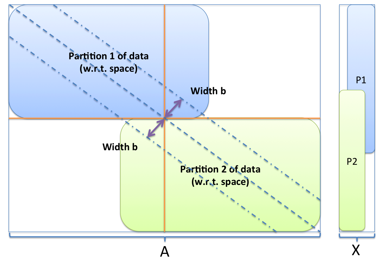
Figure 1: Banded $A$ matrix.

6.1 Efficient one-step-ahead prediction with spatially sparse models

If one observes $X_{t}$ at a given timestamp $t$, then the best linear predictor of $X_{t+1}$ is

$$\widehat{X}_{t+1}=AX_{t}.$$

Let us assume we split $A$ into a row partitioned matrix as follows:

$$A=\left[\begin{array}[]{ccccc}A_{1,0}&A_{1,1}\\ A_{2,-1}&A_{2,0}&A_{2,1}\\ &A_{3,-1}&A_{3,0}&A_{3,1}\\ &&\ddots&\ddots&A_{P-1,1}\\ &&&A_{P,-1}&A_{P,0}\end{array}\right].$$

For any $i\in\left\{1\ldots P\right\}$ let us denote $P_{i}$ the set of indices spanned by the rows of $A_{i,0}$ and $P_{i}^{+}$ the set of indices spanned by $A_{i,-1},\>A_{i,0},\>A_{i,1}$.

The class of sparse models considered above is a linear specific case belonging to the family

$$X_{t+1}=\left[\begin{array}[]{c}A_{\vartheta}^{1}\left(X_{t}^{P_{1}^{+}}\right)\\ A_{\vartheta}^{2}\left(X_{t}^{P_{2}^{+}}\right)\\ \vdots\\ A_{\vartheta}^{P-1}\left(X_{t}^{P_{P-1}^{+}}\right)\\ A_{\vartheta}^{P}\left(X_{t}^{P_{P}^{+}}\right)\end{array}\right]+\varepsilon_{t}$$

where $\left(A_{\vartheta}^{i}\right)_{i\in\left\{1\ldots P\right\}}$ is a family of functions from $\mathbb{R}^{\left|P_{i}^{+}\right|}$ onto $\mathbb{R}^{\left|P_{i}\right|}$ parametric by $\vartheta$.

An efficient unbiased estimator of the one-step-ahead predicted value can be written in a row partitioned manner:

$$\widehat{X}_{t+1}=\left[\begin{array}[]{c}\widehat{X_{t}^{P_{1}}}\\ \widehat{X_{t}^{P_{2}}}\\ \vdots\\ \widehat{X_{t}^{P_{P-1}}}\\ \widehat{X_{t}^{P_{P}}}\end{array}\right]=\left[\begin{array}[]{c}A_{\vartheta}^{1}\left(X_{t}^{P_{1}^{+}}\right)\\ A_{\vartheta}^{2}\left(X_{t}^{P_{2}^{+}}\right)\\ \vdots\\ A_{\vartheta}^{P-1}\left(X_{t}^{P_{P-1}^{+}}\right)\\ A_{\vartheta}^{P}\left(X_{t}^{P_{P}^{+}}\right)\end{array}\right].$$

In the linear case above, the time complexity of the operation is $O\left(d\times\left(2b+1\right)\right)\ll O\left(d^{2}\right)$.

6.2 Efficient sparsity leveraging Bayesian estimation

We assume that $\left(\varepsilon_{t}\right)$ is a Gaussian white noise whose precision matrix, $\Pi_{\varepsilon}=\Sigma_{\varepsilon}^{-1}$ is block diagonal with blocks corresponding to the sets of rows and columns $P_{1},\>P_{2},\ldots,P_{P}$.

$$\Pi_{\varepsilon}=\Sigma_{\varepsilon}^{-1}=\left[\begin{array}[]{ccccc}\pi_{1}&0\\ 0&\pi_{2}&0\\ &&\ddots\\ &&0&\pi_{P-1}&0\\ &&&0&\pi_{P}\end{array}\right].$$

The conditional log-likelihood of an observed process is therefore

$$\mathcal{L}\left(\vartheta,\Pi_{\varepsilon}\right)=\frac{N-1}{2}\mbox{log}\left(\mbox{det}\left(\Pi_{\varepsilon}\right)\right)-\sum_{t=1}^{N-1}\left(X_{t+1}-A_{\vartheta}\left(X_{t}\right)\right)^{T}\Pi_{\varepsilon}\left(X_{t+1}-A_{\vartheta}\left(X_{t}\right)\right).$$

Consider

$$\mathcal{L}_{t}\left(\vartheta,\Pi_{\varepsilon}\right)=\left(X_{t+1}-A_{\vartheta}\left(X_{t}\right)\right)^{T}\Pi_{\varepsilon}\left(X_{t+1}-A_{\vartheta}\left(X_{t}\right)\right)=\sum_{i,j=1}^{P}\left(X_{t+1}^{P_{i}}-A_{\vartheta}^{i}\left(X_{t}^{P_{i}^{+}}\right)\right)^{T}\Pi_{\varepsilon}^{P_{i},P_{j}}\left(X_{t+1}^{P_{j}}-A_{\vartheta}^{j}\left(X_{t}^{P_{j}^{+}}\right)\right).$$

We have assumed $\forall i\neq j,\>\Pi_{\varepsilon}^{P_{i},P_{j}}=0$, therefore

$$\mathcal{L}_{t}\left(\vartheta,\Pi_{\varepsilon}\right)=\sum_{i=1}^{P}\left(X_{t+1}^{P_{i}}-A_{\vartheta}^{i}\left(X_{t}^{P_{i}^{+}}\right)\right)^{T}\pi_{i}\left(X_{t+1}^{P_{i}}-A_{\vartheta}^{i}\left(X_{t}^{P_{i}^{+}}\right)\right)$$

and furthermore

$$\mathcal{L}\left(\vartheta,\Pi_{\varepsilon}\right)=\frac{N-1}{2}\mbox{log}\left(\mbox{det}\left(\Pi_{\varepsilon}\right)\right)-\sum_{i=1}^{P}\sum_{t=1}^{N-1}\left(X_{t+1}^{P_{i}}-A_{\vartheta}^{i}\left(X_{t}^{P_{i}^{+}}\right)\right)^{T}\pi_{i}\left(X_{t+1}^{P_{i}}-A_{\vartheta}^{i}\left(X_{t}^{P_{i}^{+}}\right)\right).$$

Let us consider we want to maximize $\mathcal{L}\left(\vartheta,\Pi_{\varepsilon}\right)$ with respect to $\vartheta$, we have

$$\nabla_{\vartheta}\mathcal{L}\left(\vartheta,\Pi_{\varepsilon}\right)=-2\sum_{i=1}^{P}\sum_{t=1}^{N-1}\left(D_{\vartheta}A_{\vartheta}^{i}\left(X_{t}^{P_{i}^{+}}\right)\right)^{T}\pi_{i}\left(X_{t+1}^{i}-A_{\vartheta}\left(X_{t}^{P_{i}^{+}}\right)\right)$$

where, letting $\left|\vartheta\right|$ denote the number of parameters in the model,

$$D_{\vartheta}A_{\vartheta}^{i}\left(X_{t}^{P_{i}^{+}}\right)=\left[\begin{array}[]{ccc}\partial_{\vartheta_{1}}A_{\vartheta}^{i}\left(X_{t}^{P_{i}^{+}}\right)&\ldots&\partial_{\Theta_{\left|\vartheta\right|}}A_{\vartheta}^{i}\left(X_{t}^{P_{i}^{+}}\right)\end{array}\right].$$

What is remarkable with these expressions is that they enable embarrassingly parallel computations provided one uses $P$ different nodes for any $i\in\left\{1\ldots P\right\}$, node $i$ holds the data corresponding to $\left(X_{t}^{P_{i}^{+}}\right)_{t\in\left\{1\ldots N\right\}}$. This is also true if one plans on using a second order method.

With a first order method, the time complexity of computing the gradient for each node is $O\left(N\times\left|\vartheta\right|\times\left|P_{i}^{+}\right|^{2}\right)$ where $\left|P_{i}^{+}\right|$ the cardinal of the overlapping partition which can be as low as $2\times b+1$. This implies that this solution is scalable with respect to the size of the model as it leverages the prior knowledge of the model’s sparsity. To the best of our knowledge, there is no equivalent computational result with the matrix inversion and Yule-Walker equation based methods above.

6.3 Gradient descent, step size and rate of convergence

This section focuses on the maximization of the conditional likelihood of a Gaussian AR process. In order to simplify notations we only consider the AR1 case. The conclusions below are trivially extended to the general case. Letting $\pi_{\varepsilon}$ the precision matrix of the process’ noise, maximizing the conditional likelihood of the process is equivalent to maximizing

$$\mathcal{L}\left(A_{1},\pi_{\varepsilon}\right)=\frac{1}{N}\sum_{t=1}^{N}\sum_{t=1}^{d}\sum_{t=1}^{d}\left(X_{t}^{i}-\sum_{k=1}^{d}A_{1}^{ik}X_{t-1}^{k}\right)\pi_{\varepsilon}^{i,j}\left(X_{t}^{j}-\sum_{l=1}^{d}A_{1}^{jl}X_{t-1}^{l}\right)$$

and

$$\frac{\partial\mathcal{L}}{\partial A_{1}^{i_{0},j_{0}}}\left(A_{1},\pi_{\varepsilon}\right)=-\frac{2}{N}\sum_{t=1}^{N}\sum_{j=1}^{d}X_{t-1}^{j_{0}}\pi_{\varepsilon}^{i_{0},j}\left(X_{t}^{j}-\sum_{l=1}^{d}A_{1}^{jl}X_{t-1}^{l}\right).$$

We consider $\pi_{\varepsilon}$ has already been estimated by $\widehat{\pi_{\varepsilon}}$. Maximizing $\mathcal{L}$ with respect to $A_{1}$ then comes down to a gradient ascent update by $\left(\frac{\partial\mathcal{L}}{\partial A_{1}^{i_{0},j_{0}}}\left(A_{1},\widehat{\pi_{\varepsilon}}\right)\right)_{i_{0},j_{0}}$. In several particular cases this update matrix takes a remarkable form:

• If $\widehat{\pi_{\varepsilon}}=I$, $\frac{\partial\mathcal{L}}{\partial A_{1}^{i_{0},j_{0}}}\left(A_{1},\widehat{\pi_{\varepsilon}}\right)=-\frac{2}{N}\sum_{t=1}^{N}X_{t-1}^{j_{0}}\left(X_{t}^{i_{0}}-\sum_{l=1}^{d}A_{1}^{i_{0}l}X_{t-1}^{l}\right)=-2\widehat{\mbox{Cov}}\left(\overrightarrow{X_{t}},X_{t}\right)$. In this case the Hessian of $A_{1}\rightarrow\mathcal{L}\left(A_{1},\widehat{\pi_{\varepsilon}}\right)$ is a block diagonal matrix whose blocks are $\widehat{\mbox{Cov}}\left(X_{t},X_{t}\right)$. Therefore finding the smallest $m$ and largest $L$ eigenvalues of $\widehat{\mbox{Cov}}\left(X_{t},X_{t}\right)$ is sufficient to compute $\frac{2}{m+L}$. This step size is of importance as it provably achieves an exponential rate of convergence to the optimum in a gradient ascent.

• If $\widehat{\pi_{\varepsilon}}$ is diagonal, $\frac{\partial\mathcal{L}}{\partial A_{1}^{i_{0},j_{0}}}\left(A_{1},\widehat{\pi_{\varepsilon}}\right)=-\frac{2}{N}\sum_{t=1}^{N}X_{t-1}^{j_{0}}\widehat{\pi_{\varepsilon}^{i_{0},j_{0}}}\left(X_{t}^{i_{0}}-\sum_{l=1}^{d}A_{1}^{i_{0}l}X_{t-1}^{l}\right)=-2\widehat{\pi_{\varepsilon}^{i_{0},j_{0}}}\widehat{\mbox{Cov}}\left(\overrightarrow{X_{t}},X_{t}\right)$. The Hessian is then the Kronecker product of $\widehat{\pi_{\varepsilon}}$ and $\widehat{\mbox{Cov}}\left(X_{t},X_{t}\right)$ which means it is sufficient to compute the smallest and largest eigenvalues of $\widehat{\pi_{\varepsilon}}$ and $\widehat{\mbox{Cov}}\left(X_{t},X_{t}\right)$ in order to find a converging step size to the gradient ascent. The rate of convergence in that case will be linear.

• In any case, a line search method also enables convergence to the maximum.

For the detail of these convergence rates we refer the reader to

7 Common access patterns, fragmentation of data, distribution of computations

The M (frequentist, average based) and Z (bayesian, maximum likelihood based) estimators above rely on similar computational needs. Namely, one computes the output of a kernel function evaluated on neighboring data and then averages the results.

7.1 Map reduce for M kernel based estimators

There is a very common computation pattern to the estimators. Frequentist estimators rely on the estimation of a covariance function. In the centered case, this can be computed by considering a finite covariance matrix which can be estimated by computing quantities

$$\widehat{\gamma_{h}^{X}}\left(\left(X_{t}\right)_{t\in\left\{1\ldots N\right\}}\right)=\frac{1}{N-h-1}\sum_{k=1}^{N-h}X_{k}X_{k+h}^{T}$$

for $h\in\left\{-H\ldots H\right\}$. This means that the vector of square matrices

$$\left(\widehat{\gamma_{h}^{X}}\left(\left(X_{t}\right)_{t\in\left\{1\ldots N\right\}}\right)\right)_{h\in\left\{-H\ldots H\right\}}$$

can be approximately estimated as

$$\frac{1}{N-\left(2h+1\right)}\ \sum_{k=h+1}^{N-h}\left(X_{k}X_{k-h}^{T},\>X_{k}X_{k-\left(h-1\right)}^{T},\ldots,\>X_{k}X_{k}^{T},\>X_{k}X_{k+1}^{T},\ldots,X_{k}X_{k+h}^{T}\right).$$

This estimator is biased but asymptotically unbiased. Computing this estimator of the auto-covariance matrix is quite straightforward with map-reduce operators. One maps the computation of the local kernel

$$\left(X_{k-h},\ldots,X_{k-1},X_{k},X_{k+1},\ldots,X_{k+h}\right)\overset{\kappa}{\rightarrow}\left(X_{k}X_{k-h}^{T},\>X_{k}X_{k-\left(h-1\right)}^{T},\ldots,\>X_{k}X_{k}^{T},\>X_{k}X_{k+1}^{T},\ldots,X_{k}X_{k+h}^{T}\right)$$

and then reduces with a sum operator prior to normalizing by $\frac{1}{N-\left(2h+1\right)}$. Such a computational schema is represented in Figure 2. This estimator is asymptotically normal with a $\frac{1}{N}$ convergence rate.

Figure 2: Example of a mapped kernel based estimation in the case of the estimation of order $H$ auto-covariance

7.2 Map reduce for Z kernel based estimators

Computing the gradient of parameters in an auto-regressive model of finite order $p$ can also be formulated in terms of a similar computational schema. For instance, when one tries to solve the conditional maximum likelihood problem for an AR model

$$\underset{A_{1},A_{2},\ldots,A_{p},\>\Theta}{\max}\sum_{t=p+1}^{N}\log f\left(\Theta,X_{t}-A_{1}X_{t-1}-\ldots-A_{p}X_{t-p}\right)$$

by a first order method, the gradient can also be computed as a sum over a large number of terms of locally computable quantities. Indeed, let $F$ be the function

$$\left(\Theta,A_{1},\ldots,A_{p}\right)\overset{F}{\rightarrow}\sum_{t=p+1}^{N}\log f\left(\Theta,X_{t}-A_{1}X_{t-1}-\ldots-A_{p}X_{t-p}\right)=\sum_{t=p+1}^{N}F_{t}\left(\Theta,X_{t}-A_{1}X_{t-1}-\ldots-A_{p}X_{t-p}\right).$$

Then, by linearity of the gradient,

$$\nabla F\left(\Theta,A_{1},\ldots,A_{p}\right)=\sum_{t=p=1}^{N}\nabla F_{t}\left(\Theta,X_{t}-A_{1}X_{t-1}-\ldots-A_{p}X_{t-p}\right).$$

For any $t\in\left\{p+1\ldots N\right\}$, computing

$$\nabla F_{t}\left(\Theta,X_{t}-A_{1}X_{t-1}-\ldots-A_{p}X_{t-p}\right)$$

only relies on data $X_{t},\ldots,X_{t-p}$.

7.3 Overlapping data

These quantities are straightforward to compute in a serial manner on a single CPU. However, when it comes to using a distributed system of computation such as Apache Spark, one has to take into account the requirement for data to be partitioned. In order to speed up the computation process and avoid the inter-node communication bottleneck one will want to mostly use a data partitioning scheme that, once loaded in the RAM of a cluster of machines, will enable embarrassingly parallel computations.

For GPU units to speed further up the process, it is also interesting to consider data partitioning as global memory units are usually slower to access than shared one. Furthermore, one will want to be able to run the computations above in an embarrassingly parallel way once appropriate parallelization steps have been undertaken.

As we explain in the following, this preparation step consists of replicating the data so as to create overlapping partitioning. The next part will explain the theoretical foundations of the scheme and how to choose its padding horizon parameter appropriately with respect to the calibration of a certain model. In particular, we introduce the fundamental data structure that has been designed to enable large scale analysis of time series: distributed overlapping blocks.

Part II A general programming paradigm for weak memory estimation

In this paragraph we will give formal definitions of the notions of weak memory from a computational standpoint. The following enables general purpose time series analysis calculus to run on partitioned data architecture in an embarrassingly parallel manner. In particular, the distributed overlapping block data structure enables partitioning with respect to both the different dimensions of a time series (different signals, sources of data) and with respect to time, which is new to the best of our knowledge. The paradigm is simple and therefore can easily be adapted to other systems. This non system specific principle of overlapping blocks is very powerful though as it enables in-RAM computations on time series with an EC2 cluster in an embarrassingly parallel way as well as GPU parallelization of time series calculus thanks to CUDA.

The package created for Apache Spark, SparkGeoTS, that follows this scheme enables time series analysis at an unprecedented scale, both in terms of density of time stamps along the time axis and in terms of very highly dimensional time series analysis. It supports data analytics for both regularly time stamped data and irregularly spaced time series. Its novelty stems from leveraging the informational properties of weak memory in ergodic time series. It is not adapted to the non-ergodic context which is not an actual shortcoming as in this case most usual estimators for time series are not even convergent.

8 Weak memory computation for estimators

The first part of this document reviewed a vast class of time series models that feature weak memory computational needs. In the following we formalize that notion. Let us consider data in the form of $\left(X_{t}\right)_{t\in\left\{0\ldots N\right\}}$.

Definition: Order $H$ weak memory estimator

An estimator $\mbox{Est}\left(\left(X_{t}\right)_{t\in\left\{0\ldots N\right\}}\right)$ features order $H$ weak memory if there exists an integer $H$ (horizon in number of steps) such that sufficient statistics for that estimator can be computed by reducing kernel computation results feeding on a data point and the neighbors of that point that are less than $H$ time steps away on the time index.

Example: Second order stationary time series

We have shown above that usual estimators for AR$(p)$ models are $p$ weak memory estimators, similarly with MA$(q)$ ($q$ weak memory) and ARMA$(p,q)$ models ($p+q$ weak memory).

9 Weak memory in time series graphs

If one considers a system in which sensors are included in a relational graph then the time series of readings produced by these sensors are naturally embedded in a graph. An example of the resulting data lattice is represented in Figure 3.

A regularly indexed time series graph is a sequence $\left(\left(X_{t}^{v}\right)_{v\in V}\right)_{t\in\left\{1\ldots N\right\}}$ where the set $V$ of vertices of the graph is tied together by a set $E$ of edges with uniform weight $1$.

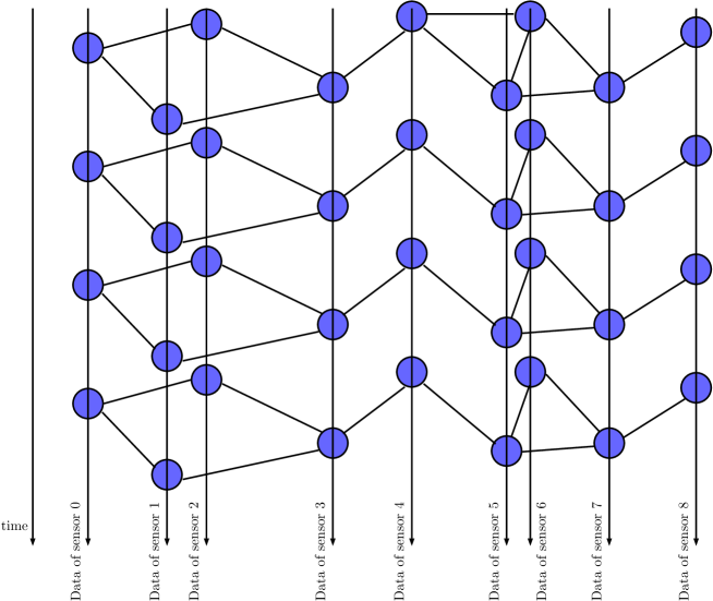
Figure 3: Sensor graph lattice

9.1 Data with regularly indexed timestamps

Definition: Order $\left(H,K\right)$ weak memory estimator

An estimator $\mbox{Est}\left[\left(\left(X_{t}^{v}\right)_{v\in V}\right)_{t\in\left\{1\ldots N\right\}}\right]$ is said to feature order $\left(H,K\right)$ weak memory if sufficient statistics can be computed by reducing kernel computations that, for each vertex state $X_{t}^{v}$, only feed on the states of neighbors that are at most $K$ hops away in the graph on a time window that does not go further than $H$ time steps away from $t_{0}$.

Example: queuing model for arterial traffic

A traffic network can be mapped to a graph where vertices represent intersections and edges correspond to roads. Such a mapping correspond to a primal whose dual graph consists of vertices modeling roads and edges accounting for the binding intersections represent. One considers a discrete model in which the state of congestion at time $t$ on vertex $v$ only depends on the state of congestion of its upstream and downstream neighbors. This assumption is very usual in traffic as soon as the discretization resolution is such that $\frac{\Delta x}{\Delta t}\leq v$ where $\Delta x$ is the length of the shortest road, $\Delta t$ the time discretization resolution and $v$ the maximum speed of vehicles in the network.

10 Embarrassingly parallel weak memory time series distributed representations

In this section we define a programming paradigm to leverage the informational structure of short memory time series in order to make their analysis distributed and embarrassingly parallel. In particular we focus on the case where both the sampling rate and the number of dimensions of the time series under consideration are high enough so that the data cannot fit in a reasonable amount of RAM on a single machine.

10.1 Very high dimensional short memory time series

Strategies have been developed to parallelize the analysis of time series on distributed clusters or high performance computers. For Apache Spark, libraries such as SparkTS and Thunder divide the time series into smaller data sets by splitting it along dimensions. This paradigm is efficient whenever each dimension has few enough timestamp for its entire data to fit a node’s RAM. Also, for multivariate analysis, it is more suitable to preserve data locality across dimensions. The statistical estimation code that should be used then needs not be aware of the partitioning scheme. What is more, there is a gain in terms of efficiency as joins on timestamps are not necessary.

In the following we devise data structures that leverage the informational properties of short memory time series in order to make their analysis embarrassingly parallel. From a design standpoint, a map-reduce programming scheme is adopted so that pre-existing estimation tools can be used with that distributed container.

10.2 The overlapping data model

Going back to the definition of short memory in time series, it is obvious now that any local operation only needs to be aware of its $H$ neighborhood. Neighborhoods are defined in terms of steps for regularly spaced data and units of time for irregularly spaced data.

Considering the data of a time series $\left(t_{i},X_{t_{i}}\right)_{i\in\left\{1\ldots kN\right\}}$ and an estimation kernel $k\left(t_{0},\left(t_{j},X_{t_{j}}\right)_{\left|t_{j}-t_{0}\right|\leq H}\right)$ (with window width $2\times H$), any estimation based on a reduced quantity of the results of this kernel can become embarrassingly parallel provided data is partitioned, partially replicated and contained in an overlapping partitioning with overlap at least $H$.

10.2.1 Map-reduce based estimation with a kernel of width $2\times H$

Let an estimator

$$\sum_{i=1}^{N}k\left(t_{0},\left(t_{j},X_{t_{j}}\right)_{\left|t_{j}-t_{0}\right|\leq H}\right)$$

where $\sum$ stands for any commutative and associative operation.

Let us assume that the data has been partitioned in $k$ partitions with an overlap of width $H$ between partitions. The computation flow is illustrated in the case of the estimation of an auto-covariance function in Figure 2. The presence of an overlap directly enables one to make that computational embarrassingly parallel with no communication needed between computational nodes holding different partitions of the data. Such a representation of data is illustrated in Figure 4.

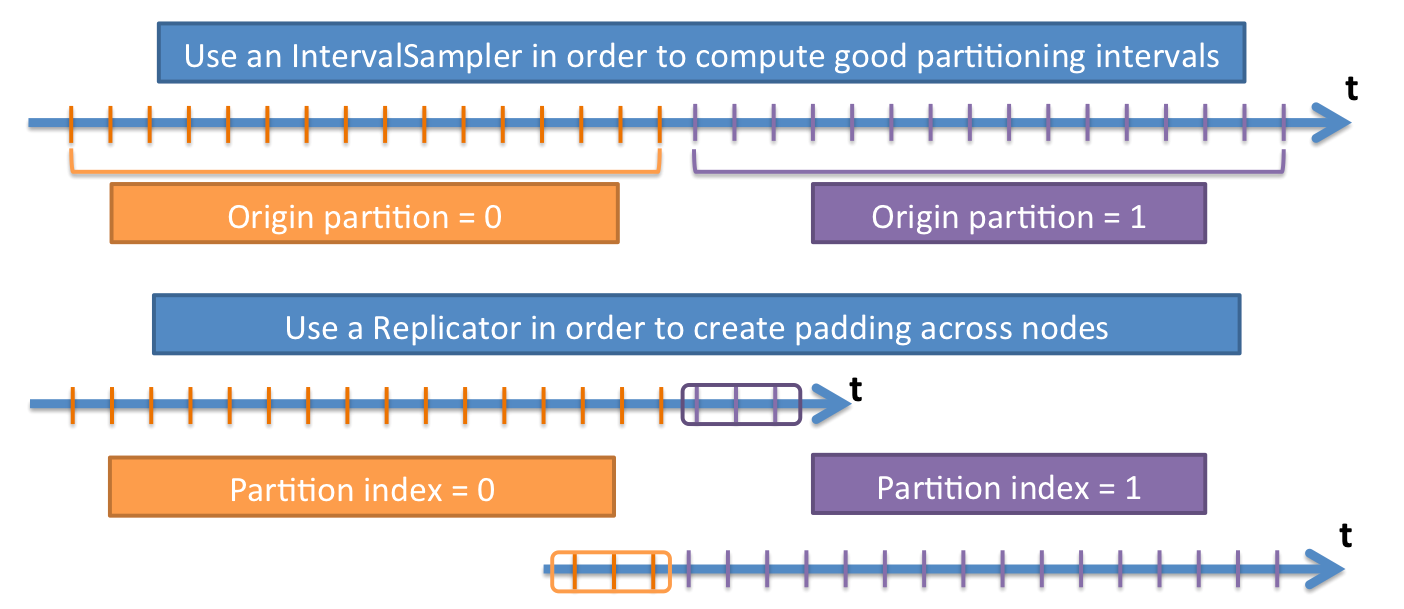
Figure 4: Overlapping distributed dataset.

10.2.2 Overlapping data set with respect to space

Time is not the only dimension along which overlapping partitioning can be computed. Obviously the scheme can be adapted to spatial meshes with regular indexing such as images. The case of data points irregularly arranged on a map falls under the same paradigm. More interesting is the case of data where no Euclidian distance is available in a straightforward way. Graphs correspond to that kind of data.

Local operations on graphs are straightforwardly defined in terms of reduced kernels provided they are only interested in the parenthood degree of the neighbors of the target. Therefore the same scheme can be adapted as illustrated in Figure 5.

Figure 5: Overlapping graph structure

10.3 Long memory case

Time series such as stock valuations on the stock market or volatility are known to feature long memory. In other words, the informational footprint of an event never completely fades away in the system. After having computed its consecutive differences, any integrated process comes down to a short memory time series. This means that the data representation paradigm above is valid in a vast range of cases. It can be extended to partially integrated processes thanks to partial differentiation provided the partial differentiation kernel is approximated by a finite support kernel.

11 Embarrassingly parallel representation of time series embedded in graphs

This section will be dedicated to finding applications of the graph overlapping paradigm above in vast systems where information flows within a sparse Dynamic Bayesian Network.

11.1 Sparse spatial dynamic bayesian network

Studying arterial network dynamics in traffic often comes down to considering the series of states of vertices (road links) bound together by intersections. In order to compute the current number of vehicles on a link, one takes into account the number of vehicles that are effectively leaving, baring the constraints of downstream occupancy capacity, to the current occupancy and adds up the number of vehicles flowing from upstream.

11.1.1 Order $\left(1,1\right)$ time and space memory Directed Acyclic Bayesian network

Such a setting is a particular instantiation of a short time and space memory time series graph. It is illustrated in Figure 6.

In such a framework, the next state of a given vertex can be computed as the result of the convolution of a kernel from its direct parents. Therefore, the overlapping data structure can be used in order to make the corresponding study embarrassingly parallel. This can be used for retrospective data analysis and simulation as well provided the same random number series are provided to edge representing identical forward state computations.

Figure 6: Order $\left(1,1\right)$ time/space memory Bayesian network (for a discretized arterial traffic model)

11.2 Cross-product of overlapping representations

In order to maintain reasonable size partitions, that is to say, partitions that can fit in the RAM of a non HPC machine, one can combine overlapping partitioning with respect to time and the corresponding time series graph in a cross-product fashion. This creates more redundant data but still provides a representation of data that enables embarrassingly parallel computations if short memory is leveraged.

If the informational structure of the data set is as presented in Figure 7, then the cross product partitioning illustrated in Figure 8 enables its embarrassingly parallel analysis.

Figure 7: Data embedded in a $\left(1,1\right)$ memory time series graph

Figure 8: Cross product of overlapping partitioning (with respect to time and space)

12 Speeding up computations on a GPU

Here we prove that the overlapping block scheme is not system specific and can be adapted to another kind of hardware: Graphical Processing Unit (SIMD systems).

12.1 Memory hierarchy

Here we focus on the memory hierarchy highlighted by Nvidia’s CUDA GPGPU language. It is possible to write data from the RAM to both the global device memory and shared memory.

The shared memory is only accessible by threads of the same block and only lives as long as a kernel execution. However, it enables one to leverage the computational power of the GPU as its bandwidth is often $100$ times that of the global memory.

Time series analysis relies on computation of local kernels in which data is mostly accessed redundantly by several threads of the same block. Therefore, it seems reasonable to try and leverage this shared memory. Each block of this memory is only accessible to the corresponding threads and the size is much less than that of the global memory (by a factor of $1000$).

We show here that overlapping blocks enable us to conduct time series analysis in a weak memory context in an embarrassingly parallel manner while leveraging the high bandwidth of shared GPU memory.

12.2 Parallel computation and overlapping blocks in shared memory for regularly spaced time series

In the following we illustrate the use of overlapping blocks on GPUs with regularly spaced time series.

We assume the data $\left(X_{t}\right)$ has been copied in the global GPU memory and one wants to execute a kernel of width $2H$ prior to conducting a reduction on the results.

Let $T_{i,j}$ the $j^{th}$ thread of the $i^{th}$ thread block. We assume blocks are of size $N_{B}+2H$ where $N_{B}$ is small enough so the shared memory of each block is not saturated. $T_{i,j}$ will copy $X_{i\left(N_{B}\right)+j}$ from the global memory (address $iN_{B}+j$) to the shared memory (local address $j$).

Then each thread with index $j\in\left\{H,\>N_{B}+H\right\}$ will compute a kernel based on data contained in local addresses corresponding to the appropriate data, namely that contained in the shared memory addresses ranging from $j-H$ to $j+H$.

Provided the kernel width outweighs the cost of the copy from the global device memory to the block’s shared memory, this provides a speed up and optimized embarrassingly parallel data analysis for weak memory systems. The flow of computations is represented in Figure 9.

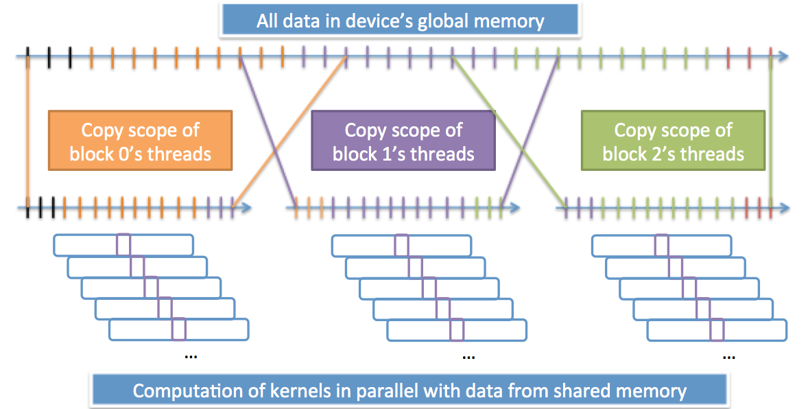
Figure 9: Overlapping block enabling shared memory used on a GPU

12.3 Parallel computation and overlapping blocks in shared memory for irregularly spaced time series

For irregularly spaced data, computations are slightly more challenging as the data that needs to be taken into account by the computation of a local kernel does not straightforwardly correspond to a range of memory addresses. However, we make a weak memory assumption that no data further away than $H$ needs to taken into account in order to compute a kernel around a datum.

One creates an overlapping partitioning of the data with $H$ overlap and baring the memory size constraint of the shared memory blocks. If the kernel considers all data points with timestamps in $\left[t-H,t+H\right]$ in order to compute its output about a datum at $t$, then letting each thread assigned with a kernel computation look backward and forward from $t$ for the first indices whose timestamps are out of range and then run the kernel convolution on the data within range solves the problem.

When kernel centers do not necessarily to data points within the data set under consideration, things get more complicated but can be made computationally efficient thanks to binary search. One may also create a skip list in the global memory of the device for each thread to access and figure out the range of the data it needs to consider. This skip list of timestamps may sit in the global memory as it will be accessed only once by each thread. Copying it to shared memory blocks would cost too much overhead.

Conclusion

In this document we have shown how weak memory models in time series analysis can be estimated and used in the context of big distributed data sets. Identifying how many lagged values are necessary to the calibration of the model the user wants to implement is a necessary preliminary step. It paves the way to building up a distributed set of overlapping partitions. This overlapping partition scheme corresponds to partitioning with respect to time which is the new contribution the present document presents. We show how this can also be extended to spatial partitioning when banded causal relationship models are being considered.
The new overlapping distributed data set presented here enables a new any-scale any-dimensional analysis of data without the need for shuffling observations between computation nodes once the appropriate data representation has been created. This provides the user with the opportunity to calibrate linear weak memory time series at scale in a reactive manner and the possibility to quickly assess how much a given model is appropriate in terms of goodness of fit and complexity. This paradigm can also be extended to the calibration of conditionally heteroscedastic models [24] as well as long memory models [25, 26]. This is the subject of ongoing work.

References

- [1] D. R. Brillinger, Time series: data analysis and theory, vol. 36. Siam, 1981.
- [2] P. J. Brockwell and R. A. Davis, Time Series: Theory and Methods. New York, NY, USA: Springer-Verlag New York, Inc., 1986.
- [3] J. D. Hamilton, “Time series analysis princeton university press,” Princeton, NJ, 1994.
- [4] A. C. Harvey and A. Harvey, Time series models, vol. 2. Harvester Wheatsheaf New York, 1993.
- [5] H. Ltkepohl, New Introduction to Multiple Time Series Analysis. Springer Publishing Company, Incorporated, 2007.
- [6] J. Dean and S. Ghemawat, “Mapreduce: simplified data processing on large clusters,” Communications of the ACM, vol. 51, no. 1, pp. 107–113, 2008.
- [7] K. Shvachko, H. Kuang, S. Radia, and R. Chansler, “The hadoop distributed file system,” in Mass Storage Systems and Technologies (MSST), 2010 IEEE 26th Symposium on, pp. 1–10, IEEE, 2010.
- [8] A. Thusoo, J. S. Sarma, N. Jain, Z. Shao, P. Chakka, N. Zhang, S. Antony, H. Liu, and R. Murthy, “Hive-a petabyte scale data warehouse using hadoop,” in Data Engineering (ICDE), 2010 IEEE 26th International Conference on, pp. 996–1005, IEEE, 2010.
- [9] M. Zaharia, M. Chowdhury, T. Das, A. Dave, J. Ma, M. McCauley, M. J. Franklin, S. Shenker, and I. Stoica, “Resilient distributed datasets: A fault-tolerant abstraction for in-memory cluster computing,” in Proceedings of the 9th USENIX conference on Networked Systems Design and Implementation, pp. 2–2, USENIX Association, 2012.
- [10] R. S. Tsay, Analysis of financial time series, vol. 543. John Wiley & Sons, 2005.
- [11] M. Mudelsee, “Climate time series analysis,” Atmospheric and, vol. 397, 2010.
- [12] S. Basu, A. Mukherjee, and S. Klivansky, “Time series models for internet traffic,” in INFOCOM’96. Fifteenth Annual Joint Conference of the IEEE Computer Societies. Networking the Next Generation. Proceedings IEEE, vol. 2, pp. 611–620, IEEE, 1996.
- [13] K. W. Hipel and A. I. McLeod, Time series modelling of water resources and environmental systems. Elsevier, 1994.
- [14] T. Hunter, T. Moldovan, M. Zaharia, S. Merzgui, J. Ma, M. J. Franklin, P. Abbeel, and A. M. Bayen, “Scaling the mobile millennium system in the cloud,” in Proceedings of the 2nd ACM Symposium on Cloud Computing, p. 28, ACM, 2011.
- [15] M. Franklin et al., “Mllib: A distributed machine learning library,” NIPS Machine Learning Open Source Software, 2013.
- [16] J. Durbin and S. J. Koopman, Time series analysis by state space methods. No. 38, Oxford University Press, 2012.
- [17] S. Boyd and L. Vandenberghe, Convex optimization. Cambridge university press, 2004.
- [18] D. P. Bertsekas, “Nonlinear programming,” 1999.
- [19] F. M. Callier and C. A. Desoer, Linear system theory. Springer Science & Business Media, 2012.
- [20] H. Kantz and T. Schreiber, Nonlinear time series analysis, vol. 7. Cambridge university press, 2004.
- [21] J. Fan and Q. Yao, Nonlinear time series: nonparametric and parametric methods. Springer Science & Business Media, 2003.
- [22] Straumann and T. Mikosch, “Estimation in conditionally heteroscedastic time series models,” tech. rep., Lecture Notes in Statist. 181, 2005.
- [23] H. Akaike, “Block toeplitz matrix inversion,” SIAM Journal on Applied Mathematics, vol. 24, no. 2, pp. 234–241, 1973.
- [24] R. Lund, “Estimation in conditionally heteroscedastic time series models,” Journal of the American Statistical Association, vol. 101, no. 475, p. 1319, 2006.
- [25] P. Doukhan, G. Oppenheim, and M. S. Taqqu, Theory and applications of long-range dependence. Springer Science & Business Media, 2003.
- [26] B. B. Mandelbrot, Fractals and Scaling in Finance: Discontinuity, Concentration, Risk. Selecta Volume E. Springer Science & Business Media, 2013.