mplrs: A scalable parallel vertex/facet enumeration code

Abstract

We describe a new parallel implementation, mplrs, of the vertex enumeration code lrs that uses the MPI parallel environment and can be run on a network of computers. The implementation makes use of a C wrapper that essentially uses the existing lrs code with only minor modifications. mplrs was derived from the earlier parallel implementation plrs, written by G. Roumanis in C++ which runs on a shared memory machine. By improving load balancing we are able to greatly improve performance for medium to large scale parallelization of lrs. We report computational results comparing parallel and sequential codes for vertex/facet enumeration problems for convex polyhedra. The problems chosen span the range from simple to highly degenerate polytopes. For most problems tested, the results clearly show the advantage of using the parallel implementation mplrs of the reverse search based code lrs, even when as few as 8 cores are available. For some problems almost linear speedup was observed up to 1200 cores, the largest number of cores tested.

Keywords: vertex enumeration, reverse search, parallel processing
Mathematics Subject Classification (2000) 90C05

1 Introduction

The vast majority of mathematical programming software was designed and implemented for the prevalent computers of the last century, which generally had single processors. Improvements in algorithmic design and processor speed, in roughly equal measure, led to enormous speed-ups allowing increasingly large problems to be solved in reasonable time. These legacy computer codes are sophisticated and extremely robust, having been extensively tested on a wide range of platforms and applications. Previously, parallel processing was limited largely to expensive supercomputers. In recent years the situation has changed radically; increases in processor speed have been replaced by the ubiquitousness of multicore processors. Desktop computers usually include at least four CPU cores and relatively inexpensive compute servers provide 64 cores in a shared memory machine. Networks of such computers readily provide hundreds of available cores. Unfortunately, very little legacy software for mathematical programming can make effective use of this hardware.

Some algorithms, such as those based on the simplex method, seem inherently sequential and will require new ideas to exploit large scale parallel processing. Others, such as integer programming via branch and cut, are basically tree searches that should benefit greatly from parallelism. For example, the Concorde code for the travelling salesman problem [3, 4] used large scale parallelism to solve extremely large problems to optimality over a distributed network. General integer programming solvers such as CPLEX [42] and Gurobi [35] also make use of multicore and distributed computing. A computational study using Gurobi is contained in Koch et al. [44]. Using a shared memory machine, they report speedups of roughly 9 times with 32 cores and 25 times with 128 cores for integer programming instances tested. Using a distributed system with 8000 cores they report an estimated speedup of approximately 800 times. However, tests by Carle [19] show that results may be very disappointing if some processors are considerably slower than others, even with only 4 or 8 processors. Much work clearly needs to be done in this area.

In this paper we report on the parallelization of lrs, a tree search algorithm for the vertex/facet enumeration problem. The method we developed has the following features which are discussed in detail below: (a) there is little modification to a complex legacy code; (b) the parallelism is applied only in a wrapper; (c) the subproblems are not interrupted; (d) there is no communication between these threads; and (e) it works on both shared-memory and distributed systems with essentially no user intervention required. We also report computational results on a variety of problems and hardware that show near linear speedups, in some cases up to 1200 processors.

Vertex/facet enumeration problems find applications in many areas, of which we list a few here. Early examples include computing the facets of correlation/cut polyhedra by physicists (see, e.g., [21, 26]) and current research in this area relates to detecting quantum behaviour in computers such as D-Wave. Research on facets of travelling salesman polytopes leads to important advances in branch-and-cut algorithms, see, e.g., [4]. For example, Chvátal local cuts are derived from facets of small TSPs and this idea is also seen in the small instance relaxations of Reinelt and Wenger [55]. Vertex enumeration is used to compute all Nash equilibria of bimatrix games and a code for this based on lrs is found at [6]. Vertex enumeration may be a last resort for minimizing extremely complicated concave functions. See, for example, Chapter 3 of Horst et al. [40]. This application shows the advantage of getting the output as a stream, most of which can be immediately discarded. When doing facet enumeration lrs automatically computes the volume of the polytope using much less memory than other methods, such as those described in [30].

The remainder of the paper is organised as follows. We begin by introducing related work in Section 2 and then proceed to background on vertex enumeration, reverse search, lrs and plrs in Section 3. This is followed in Section 4 by a discussion of various parallelization strategies that could be employed to manage the load balancing problem. In Section 5 we discuss the implementation of mplrs and describe its features. In Section 6 we give some test results on a wide range of inputs, comparing 7 codes: cddr+, normaliz, PORTA, ppl_lcdd, lrs, plrs and mplrs and present an analysis of our findings where we see that mplrs scales further than other vertex enumeration codes. Finally in the conclusion we compare our results with those obtained for parallel integer programming and discuss the wider applicability of our research.

2 Related Work

We begin by reviewing the available algorithms and codes for vertex enumeration, focusing in particular on parallel codes. Codes for this problem were recently compared by Assarf et al. [5], however they focus primarily on sequential codes and therefore utilize comparatively easy instances. Then we introduce work on parallel reverse search, and also work on other parallel search problems that may appear related to mplrs.

There are basically two algorithmic approaches to the vertex enumeration problem: the Fourier-Motzkin double description method (see, e.g., [61]) and pivoting methods such as Avis-Fukuda reverse search [10] which enumerates all nodes of a tree. The double description method involves inserting the half spaces from the H-representation sequentially and updating the list of vertices that they span. Readily available codes for this method include cddr+ [31], normaliz [52], ppl_lcdd [14] and PORTA [22]. Although this sequential method did not seem easy to parallelize, it was recently achieved and implemented in normaliz. This breakthrough for the double description method involves a new technique called pyramidal decomposition [18]. This decomposition is not equivalent to a standard polyhedral decomposition and is much less costly to compute. We include experimental results for normaliz in Section 6.

2.1 lrs and parallelization

The reverse search method for vertex enumeration was implemented as lrs [6, 7]. From the outset it was realized that reverse search was eminently suitable for parallelization. Marzetta developed the first parallel reverse search code using his ZRAM parallelization platform [17, 48], and implemented the first parallel vertex enumeration code, prs, using this generic reverse search framework. Load balancing is performed using a variant of what is now known as job stealing. Application codes, such as lrs, were embedded into ZRAM itself leading to problems of maintenance as the underlying codes evolved. Although prs is no longer distributed and was based on a now obsolete version of lrs, it clearly showed the potential for large speedups of reverse search algorithms. Some limited experimental results for vertex enumeration are given in [17] and these are discussed in Section 6.3.

The lrs code is rather complex and has been under development for over twenty years incorporating a multitude of different functions. It has been used extensively and its basic functionality is very stable. Directly adding parallelization code to such legacy software is extremely delicate and can easily produce bugs that are difficult to find. A high level wrapper avoids this problem by implementing the parallelization as a separate layer with very few changes to lrs itself. This allows the independent development of both parallelization ideas and basic improvements in the underlying code, both of which stay up to date. In return for this flexibility there are certain overheads that we discuss later. However, the focus on lrs and reverse search minimizes the number of modifications required compared to using a general framework like ZRAM, and also allows the use of a load balancing technique that is both simple and efficient for such codes.

The concept of a high level wrapper along these lines was tested by a shell script, tlrs, developed by White in 2009. Here the parallelization was achieved by scheduling independent lrs processes for subtrees via the shell. Although good speedups were obtained, several limitations of this approach materialized as the number of processors available increased. In particular job control becomes a major issue: there is no single controlling process.

To overcome these limitations the first author and Roumanis developed plrs [13]. This code is a C++ wrapper that compiles in the original lrslib library essentially maintaining the integrity of the underlying lrs code. The parallelization was achieved by multithreading using the Boost library and was designed to run on shared memory machines with little user interaction. Experience with the plrs code showed good speedups with up to about 16 cores, then reduced performance after that. The goal of mplrs was to solve this load balancing problem and to move to a distributed environment which could contain hundreds or thousands of processors.

The differences between mplrs and plrs are described in Section 3.3. While prs is able to run on distributed systems using the MPI layer in ZRAM, there are many differences between prs and mplrs. In particular, prs uses a very different strategy for load balancing where splitting work is distinct from performing work, splitting is computationally expensive, and is targeted at cases with comparatively regular search trees (see Section 6.3.2 of [48]). This is because the node descriptions are quite large (see Section 4.3.1 of [48]), and so it tries to minimize the number of subproblems stored in memory. mplrs uses much smaller node descriptions (the cobasis) and a very different strategy for load balancing, where splitting and performing work are not distinct. This budgeted tree search results in the much better scaling and performance of mplrs. Many other differences between prs and mplrs are due to the age of prs and the fact that it is no longer available or maintained.

2.2 Other parallel codes

The reverse search framework in ZRAM was also used to implement a parallel code for certain quadratic maximization problems [28]. In a separate project, Weibel [58] developed a parallel reverse search code to compute Minkowski sums. This C++ implementation runs on shared memory machines and he obtains linear speedups with up to 8 processors, the largest number reported.

ZRAM is a general-purpose framework that is able to handle a number of other applications, such as branch-and-bound and backtracking, for which there are by now a large number of competing frameworks. Recent papers by Crainic et al. [25], McCreesh et al. [50] and Herrera et al. [38] describe over a dozen such systems. While branch-and-bound may seem similar to reverse search enumeration, there are fundamental differences. In enumeration it is required to explore the entire tree whereas in branch-and-bound the goal is to explore as little of the tree as possible until a desired node is found. The bounding step removes subtrees from consideration and this step depends critically on what has already been discovered. Hence the order of traversal is crucial and the number of nodes evaluated varies dramatically depending on this order. Sharing of information is critical to the success of parallelization. Similar complications exist in parallel SAT solving [37] and parallel game tree search [41]. These issues do not occur in reverse search enumeration, and so a much lighter wrapper is possible.

Relevant to the heaviness of the wrapper and amount of programming effort required, a comparison of three frameworks is given in [38]. The first, Bob++ [27], is a high level abstract framework, similar in nature to ZRAM, on top of which the application sits. This framework provides parallelization with relatively little programming effort on the application side and can run on a distributed network. The second, Threading Building Blocks (TBB) [54], is a lower level interface providing more control but also considerably more programming effort. It runs on a shared memory machine. The third framework is the Pthread model [20] in which parallelization is deep in the application layer and migration of threads is done by the operating system. It also runs on a shared memory machine. All of these methods use job stealing for load balancing [16]. In [38] these three approaches are applied to a global optimization algorithm. They are compared on a rather small setup of 16 processors, perhaps due to the shared memory limitation of the last two approaches. The authors found that Bob++ achieved a disappointing speedup of about 3 times, considerably slower than the other two approaches which achieved near linear speedup. Other frameworks include CHiPPS [60] for parallel tree search and MW [32], which uses the HTCondor framework. MW can be used to parallelize existing applications using the master-worker paradigm; one such application was to quadratic assignment problems [2].

Computational tasks that can be divided into subproblems which can be solved independently with no communication are often called embarrassingly parallel [59]. Many such problems involve processing an enormous amount of data that can easily be divided, one prominent example being the SETI@home project [1]. A recent approach to parallel constraint solvers [47] (where the input and output are comparatively small) uses this as inspiration and initially creates a large number of subproblems that are then solved in parallel. Other approaches to creating an initial (hopefully balanced) decomposition of the input include cube-and-conquer [39], which uses a lookahead SAT solver to split the original problem into many subproblems that are solved in parallel by CDCL solvers, and applying machine learning techniques to parallel AND/OR branch-and-bound [53]. Self-splitting [29] is a technique for minimizing communication when the subproblem descriptions are large. There, each worker performs an identical split of the original problem and then follows some deterministic rule to decide which portions belong to it. This is not particularly appropriate in our case, where subproblem descriptions are small and the major concern is that subproblem difficulty is highly unbalanced.

Another way to deal with the problem posed by subproblems of varying difficulties is dynamic load balancing, where one can split difficult subproblems during the computation. Work stealing [16] is one well-known approach where free workers can steal portions of work from busy workers.

Parallel search has a long history and many applications [34]. Topics related to this paper include load balancing techniques [45, 46] and estimating the difficulty of subproblems. The general idea of developing a lightweight parallel wrapper and reusing sequential code with minimal changes has been applied in many areas, including mixed integer programming [56] and SAT solving [15].

Parallel programming is almost as old as programming itself and there is a wealth of literature on the subject which we can not cover here. For a modern introduction the reader is referred to Mattson et al. [49]. Generally, much attention is given to machine architecture, communications between processes, data sharing, synchronization, interrupts, load balancing and so on. This is essential knowledge for building and implementing a parallel algorithm from scratch. However our aim was essentially different. In return for some computational overhead, we would like to use existing sequential code with only minor modifications. In particular, this eliminates the need for considering most of these topics. The main issue that remains is load balancing, a topic we discuss in detail throughout the paper.

3 Background

3.1 The vertex/facet enumeration problem

The vertex enumeration problem is described as follows. Given an $m\times d$ matrix $A=(a_{ij})$ and an $m$ dimensional vector $b$, a convex polyhedron, or simply polyhedron, $P$ is defined as:

$$P=\{x\in\mathbb{R}^{d}:b+Ax\geq 0\}.$$ (1)

This description of a polyhedron is known as an H-representation. A polytope is a bounded polyhedron. For simplicity in this article we will assume that the input data $A,b$ defines a polytope which has dimension $d$, i.e. it is full dimensional. For this it is necessary that $m>d$. A point $x\in P$ is a vertex of $P$ if and only if it is the unique solution to a subset of $d$ inequalities from (1) solved as equations. Such a subset of inequalities is called a basis.

The vertex enumeration problem is to output all vertices of a polytope $P$. This list of vertices gives us a V-representation of $P$. The reverse transformation, called the facet enumeration problem, takes a V-representation and computes its H-representation. The two problems are computationally equivalent via polarity. A polytope is called simple if each vertex is described by a single basis and simplicial if each facet contains exactly $d$ vertices. A vertex enumeration problem for a simple polytope is called non-degenerate as is a facet enumeration problem for a simplicial polytope. Other such problems are called degenerate. Since the two problems are equivalent, we will consider only the vertex enumeration problem in what follows.

One of the features of these types of enumeration problems is that the output size varies widely for given parameters $m$ and $d$. It is known that up to scaling by constants, each full dimensional polytope has a unique non-redundant $H$ and $V$ representation. For the bounds given next we assume such representations. For positive integers $m>d$ let

$$f(m,d)=\binom{m-\left\lfloor\frac{d+1}{2}\right\rfloor}{m-d}+\binom{m-\left\lfloor\frac{d+2}{2}\right\rfloor}{m-d}\,.$$ (2)

McMullen’s Upper Bound Theorem (see, e.g., [61]) states that for a polytope whose $H$-representation has parameters $m>d$ the maximum number of vertices it can have is $f(m,d)$. This bound is tight and is achieved by the class of cyclic polytopes. By inverting the formula and using polarity we can get lower bounds on the number of vertices of a polytope. We have:

$$\min\{t:m\leq f(t,d)\}~{}\leq~{}|V|~{}\leq~{}f(m,d)\,.$$ (3)

The first inequality follows because a polytope with fewer than this number of vertices must have less than $m$ facets. For example, suppose $m=40$ and $d=20$. Then we have $22\leq|V|\leq 40,060,020$.

Pivoting methods compute the bases of a polytope and this number can be much larger than the upper bound in (3). However, as described in the next subsection, lrs uses lexicographic pivoting which is equivalent to a symbolic perturbation of the polytope into a simple polytope. Hence $f(m,d)$ is a tight upper bound on the number of bases computed. Since we only require each vertex once, highly degenerate polytopes will cause large overhead for pivoting methods.

3.2 Reverse search and lrs

Reverse search is a technique for generating large, relatively unstructured, sets of discrete objects. We give an outline of the method here and refer the reader to [10, 11] for further details. In its most basic form, reverse search can be viewed as the traversal of a spanning tree, called the reverse search tree $T$, of a graph $G=(V,E)$ whose nodes are the objects to be generated. Edges in the graph are specified by an adjacency oracle, and the subset of edges of the reverse search tree are determined by an auxiliary function, which can be thought of as a local search function $f$ for an optimization problem defined on the set of objects to be generated. One vertex, $v^{*}$, is designated as the target vertex. For every other vertex $v\in V$, repeated application of $f$ must generate a path in $G$ from $v$ to $v^{*}$. The set of these paths defines the reverse search tree $T$, which has root $v^{*}$.

A reverse search is initiated at $v^{*}$, and only edges of the reverse search tree are traversed. When a node is visited the corresponding object is output. Since there is no possibility of visiting a node by different paths, the nodes are not stored. Backtracking can be performed in the standard way using a stack, but this is not required as the local search function can be used for this purpose. This implies two critical features that are essential for effective parallelization. Firstly, it is not necessary to store more than one node of the tree at any given time and no database is required for visited nodes. Secondly, it is possible to restart the enumeration process from any given node in the tree using only a description of this one node. This contrasts with standard depth first search algorithms for which restart is only possible with a complete database of visited nodes as well as the backtrack stack to the root of the search tree.

In the basic setting described here a few properties are required. Firstly, the underlying graph $G$ must be connected and an upper bound on the maximum vertex degree, $\Delta$, must be known. The performance of the method depends on $G$ having $\Delta$ as low as possible. The adjacency oracle must be capable of generating the adjacent vertices of some given vertex $v$ sequentially and without repetition. This is done by specifying a function $\textrm{Adj}(v,j)$, where $v$ is a vertex of $G$ and $j=1,2,\ldots,\Delta$. Each value of $\textrm{Adj}(v,j)$ is either a vertex adjacent to $v$ or null. Each vertex adjacent to $v$ appears precisely once as $j$ ranges over its possible values. For each vertex $v\neq v^{*}$ the local search function $f(v)$ returns the tuple $(u,j)$ where $v=\textrm{Adj}(u,j)$ such that $u$ is $v$’s parent in $T$. Pseudocode is given in Algorithm 1. Note that the vertices are output as a continuous stream. For convenience later, we do not output the root vertex $v^{*}$ in the pseudocode shown.

1:procedure rs($v^{*}$, $\Delta$, Adj, $f$)

2:     $v\leftarrow v^{*}$   $j\leftarrow 0$   $\mathit{depth}\leftarrow 0$

3:     repeat

4:         while $j<\Delta$ do

5:              $j\leftarrow j+1$

6:              if $f(\textrm{Adj}(v,j))=v$ then $\triangleright$ forward step

7:                  $v\leftarrow\textrm{Adj}(v,j)~{}~{}~{}~{}~{}$

8:                  $j\leftarrow 0$

9:                  $\mathit{depth}\leftarrow\mathit{depth}+1$

10:                  output $v$

11:              end if

12:         end while

13:         if $\mathit{depth}>0$ then $\triangleright$ backtrack step

14:              $(v,j)\leftarrow f(v)$

15:              $\mathit{depth}\leftarrow\mathit{depth}-1$

16:         end if

17:     until $\mathit{depth}=0$ and $j=\Delta$

18:end procedure

Algorithm 1 Generic Reverse Search

To apply reverse search to vertex enumeration we first make use of dictionaries, as is done for the simplex method of linear programming. To get a dictionary for (1) we add one new nonnegative variable for each inequality:

$$x_{d+i}=b_{i}+\sum_{j=1}^{d}{a_{ij}x_{j}},~{}~{}x_{d+i}\geq 0~{}~{}~{}i=1,2,\ldots,m.$$

These new variables are called slack variables and the original variables are called decision variables.

In order to have any vertex at all we must have $m\geq d$, and normally $m$ is significantly larger than $d$, allowing us to solve the equations for various sets of variables on the left hand side. The variables on the left hand side of a dictionary are called basic, and those on the right hand side are called non-basic or, equivalently, co-basic. We use the notation $B=\{i:{x_{i}}\mbox{ is basic}\}$ and $N=\{j:{x_{j}}\mbox{ is co-basic}\}$.

A pivot interchanges one index from $B$ and $N$ and solves the equations for the new basic variables. A basic solution from a dictionary is obtained by setting $x_{j}=0$ for all $j\in N$. It is a basic feasible solution (BFS) if $x_{j}\geq 0$ for every slack variable $x_{j}$. A dictionary is called degenerate if it has a slack basic variable $x_{j}=0$. As is well known, each BFS defines a vertex of $P$ and each vertex of $P$ can be represented as one or more (in the case of degeneracy) BFSs.

Next we define the relevant graph $G=(V,E)$ to be used in Algorithm 1. Each node in $V$ corresponds to a BFS and is labelled with the cobasic set $N$. Each edge in $E$ corresponds to a pivot between two BFSs. Formally we may define the adjacency oracle as follows. Let $B$ and $N$ be index sets for the current dictionary. For $i\in B$ and $j\in N$

$$\textrm{Adj}(N,i,j)=\left\{\begin{array}[]{ll}N\setminus\{j\}\cup\{i\}&\mbox{if this gives a feasible dictionary}\\ \emptyset&\mbox{otherwise\,.}\\ \end{array}\right.$$

A target $v^{*}$ for the reverse search is found by solving a linear program over this dictionary with any objective function. A new objective function is then chosen so that the optimum dictionary is unique and represents $v^{*}$. lrs uses Bland’s least subscript rule for selecting the variable which enters the basis and a lexicographic ratio test to select the leaving variable. The lexicographic rule simulates a simple polytope which greatly reduces the number of bases to be considered. We initiate the reverse search from the unique optimum dictionary. For more details see the technical description at [6]. lrs is an implementation of Algorithm 1 in exact rational arithmetic using $\textrm{Adj},f,\mbox{ and }v^{*}$ as just described.

3.3 Parallelization and plrs

The development of mplrs started from our experiences with plrs, with the goal of scaling past the limits of other vertex enumeration codes while using the existing lrs code with only minor modifications. The details of plrs are described in [13]; here we give a generic description of the parallelization which is by nature somewhat oversimplified. We will use as an example the tree shown in Figure 1 which shows the first two layers of the reverse search tree for the problem mit, an 8-dimensional polytope with 729 facets that will be described in Section 6.1. The weight on each node is the number of nodes in the subtree that it roots. The root of the tree is in the centre and its weight shows that the tree contains 1375608 nodes, the number of cobases generated by lrs. At depth 2 there are 35 nodes but of these, just the four underlined nodes contain collectively about 58% of the total number of tree nodes.

Figure 1: Number of nodes in subtrees at depth 2 for mit

The method implemented in plrs proceeds in three phases. In the first phase, sometimes called ramp-up in the parallel processing literature, we generate the reverse search tree $T$ down to a fixed depth, $\mathit{init\_depth}$, reporting all nodes to the output stream. In addition, the nodes of the tree with depth equal to $\mathit{init\_depth}$ which are not leaves of $T$ are stored in a list $L$.

In the second phase we schedule subtree enumeration for nodes in $L$ using a user-specified parameter $\mathit{max\_threads}$ to limit the number of parallel processes. For subtree enumeration we use lrs with a slight modification to its earlier described restart feature. Normally, in a restart, lrs starts at a given restart node at its given depth and computes all remaining nodes in the tree $T$. The simple modification is to supply a depth of zero with the restart node so that the search terminates when trying to backtrack from this node.

When the list $L$ becomes empty we move to Phase 3, sometimes called ramp-down, in which the threads terminate one by one until there are no more running and the procedure terminates. In both Phase 2 and Phase 3 we make use of a collection process which concatenates the output from the threads into a single output stream. It is clear that the only interaction between the parallel threads is the common output collection process. The only signalling required is when a thread initiates or terminates a subtree enumeration.

Let us return to the example in Figure 1. Suppose we set $\mathit{init\_depth}=2$ and $\mathit{max\_threads}=12$. A total of 35 nodes are found at this depth. 34 are stored in $L$ and the other, being a leaf, is ignored. The first 12 nodes are removed from $L$ and scheduled on the 12 threads. Each time a subtree is completely enumerated the associated thread receives another node from $L$ and starts again. When $L$ is empty the thread is idle until the entire job terminates. To visualize the process refer to Figure 2. In this case we have set $\mathit{init\_depth}=3$ to obtain a larger $L$. The vertical axis shows thread usage and the horizontal axis shows time. Phase 1 is so short - less than one second - that it does not appear. Phase 2 lasts about 50 seconds, when all 12 threads are busy. Phase 3 lasts the remaining 70 seconds as more and more threads become idle. If we add more cores, only Phase 2 will profit. Even with very many cores the running time will not drop below 70 seconds and so this technique does not scale well. In comparing Figures 1 and 2 we see that the few large subtrees create an undesirably long Phase 3. Going to a deeper initial depth helps to some extent, but this eventually creates an extremely long list $L$ with subsequent increase in overhead (see [13] for more details). Nevertheless plrs performs very well with up to about 32 parallel threads, as we will see in Section 6.

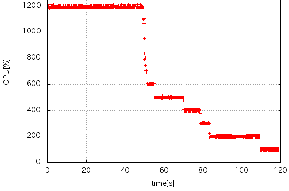
Figure 2: Processor usage by plrs on problem mit on a 12 core machine, $\mathit{init\_depth}=3$

In analyzing this method we observe that in Phase 1 there is no parallelization, in Phase 2 all available cores are used, and in Phase 3 the level of parallelization drops monotonically as threads terminate. Looking at the overhead compared with lrs we see that this almost entirely consists of the amount of time required to restart the reverse search process. In this case it requires the time to pivot the input matrix to a given cobasis, which is not negligible. However a potentially greater cost occurs when $L$ is empty and threads are idle. As the number of available processors increase this cost goes up, but the overhead of restarting remains the same, for given fixed $\mathit{init\_depth}$. This leads to conflicting issues in setting the critical $\mathit{init\_depth}$ parameter. A larger value implies that:

• only a single thread is working for a longer time,

• the list $L$ will typically be larger requiring more overhead in restarts but,

• the time spent in Phase 3 will typically be reduced.

The success in parallelization clearly depends on the structure of the tree $T$. In the worst case it is a path and no parallelization occurs in Phase 2. Therefore in the worst case we have no improvement over lrs. In the best case the tree is balanced so that the list $L$ can be short reducing overhead and all threads terminate at more or less the same time. Success therefore heavily depends on the structure of the underlying enumeration problem.

4 Load Balancing Strategies

plrs generates subproblems in an initial phase based on a user supplied $\mathit{init\_depth}$ parameter. This tends to perform best on balanced trees which, in practice, seem rather rare. In plrs, workers (except the initial Phase 1 worker) always finish the subproblem that they are assigned. However, there is no guarantee that subproblems have similar sizes and as we have seen they can differ dramatically. As we saw earlier, this can lead to a major loss of parallelism after the queue $L$ becomes empty. Load balancing is the efficient distribution of work among a number of processors and is a well-studied area of parallel computation, see for example Shirazi et al. [57]. The constraints of our parallelization approach described in the Introduction, such as no interrupts or communication between subprocesses, greatly limits the methods available. In this section we discuss various strategies we tried in developing mplrs. In particular, we focus on:

• estimating the size of subproblems to improve scheduling and create reasonably-sized problems,

• dynamic creation of subproblems, where we can split subproblems at any time instead of only during the initial phase,

• using budgets for workers, who return after exploring a budgeted number of nodes adding unfinished subproblems to $L$.

4.1 Subtree Estimation

A glance at Figure 1 shows the problem with using a fixed initial depth to generate the subtrees for $L$: the tree mass is concentrated on very few nodes. Of course, increasing $\mathit{init\_depth}$ would decrease the size of the large subtrees. However, the subtrees can still be unbalanced at the new depth and this also increases the number of jobs in $L$, increasing the restart overhead. Since lrs has the capability to estimate subtree size we tried two approaches using that: priority scheduling and iterative deepening.

Estimation is possible for vertex enumeration by reverse search using Hall-Knuth estimation [36]. From any node a child can be chosen at random and by continuing in the same way a random path to a leaf is constructed. This leads to an unbiased estimate of the subtree size from the initial node. Various methods lead to lower variance, see [8].

The first use of estimation we tried was in priority scheduling. Although finding a schedule that minimizes the total time to complete all work is NP-hard, good heuristics are available. One such heuristic is the list decreasing heuristic, analyzed by Graham [33], that schedules the jobs in decreasing order by their execution time. Referring again to Figure 1 we see that we should schedule those four heaviest subtrees at the start of Phase 2. Since we do not have the exact values of the subtree sizes we decided to use the estimation function as a proxy. We then scheduled jobs from $L$ in a list decreasing manner by estimated tree size.

A second idea we tried was iterative deepening. We start by setting a threshold value, say $k$, for maximum estimated subtree size. Once a node at $\mathit{init\_depth}$ is encountered an estimate of its subtree size is made. If this exceeds $k$ then we continue to the next layer of the tree and estimate the subtree sizes again, repeatedly going deeper in the tree for subtrees whose estimates exceed $k$. In this way all nodes returned to $L$ will have estimated subtree sizes smaller than $k$.

The results from these two approaches were mixed. There are two negative points. One is that Hall-Knuth estimates have very high variance, and the true value tends to be larger than the estimate in probability. So very large subtrees receiving small estimates would not be scheduled first in priority scheduling and would not be broken up by iterative deepening. Secondly, the nodes visited during the random probes represent overhead, as these nodes will all be visited again later. In order to improve the quality of the estimate a large number of probes need to be made, increasing this overhead.

Nevertheless this seems to be an interesting area of research. Newer more reliable estimation techniques that do not result in much overhead, such as the on-the-fly methods of [24] and [43], may greatly improve the effectiveness of these approaches.

4.2 Dynamic Creation of Subproblems

As we saw in Section 3.3, plrs creates new subproblems only during the initial phase. We can think in terms of one boss, who creates subproblems in Phase 1, and a set of workers who start work in Phase 2 and each works on a single subproblem until it is completed. However, there is no reason why an individual worker cannot send some parts of its search tree back to $L$ without exploring them.

A simple example of this is to implement a $\mathit{skip}$ parameter. This is set at some integer value $t>1$ and subtrees rooted at every $t$-th node explored are sent back to $L$ without exploration. The boss can set the $\mathit{skip}$ parameter dynamically when allocating work from $L$. If $L$ is getting dangerously small, then a small value is set. Conversely if $L$ is very large an extremely large value is set.

We implemented this idea but did not get good results. When the $\mathit{skip}$ parameter is set then all subtrees are split into smaller pieces, even the small subtrees, which is undesirable. When $\mathit{skip}$ is too small, the list $L$ quickly becomes unmanageably large with very high overhead. It seemed hard for the boss to control the size of $L$ by varying the size of the parameter, due to the delay incurred before the new parameter propagated to all the workers.

4.3 Budgeted Subproblems

The final and most successful approach involved limiting the amount of work a worker could do before being required to quit. Each worker is given a budget which is the maximum number of nodes that can be visited. Once this budget is exceeded the worker backtracks to the root of its subtree returning all unfinished subproblems. These consist of all unexplored children of nodes in the backtrack path. This has several advantages. Firstly, if the subtree has size less than the budget (typically 5000 nodes in practice) then the entire subtree is evaluated without additional creation of overhead. Secondly, each large subtree automatically gets split up. By including all unexplored subtrees back to the root a variable number of jobs will be added to $L$. A giant subtree will be split up many times. For example, the subtree with 308626 nodes in Figure 1 will be split over 600 times, providing work for idle workers. We can also change the budget dynamically to obtain different effects. If the budget is set to be small we immediately create many new jobs for $L$. If $L$ grows large we can increase the budget: since most subtrees will be below the threshold the budget is not used up and new jobs are not created.

Budgeting can be introduced to the generic reverse search procedure of Algorithm 1 as follows. When calling the reverse search procedure we now supply three additional parameters:

• $\mathit{start\_vertex}$ is the vertex from which the reverse search should be initiated and replaces $v^{*}$,

• $\mathit{max\_depth}$ is the depth at which forward steps are terminated,

• $\mathit{max\_cobases}$ is the number of nodes to generate before terminating and reporting unexplored subtrees.

Both $\mathit{max\_depth}$ and $\mathit{max\_cobases}$ are assumed to be positive, for otherwise there is no work to do. The modified algorithm is shown in Algorithm 2.

1:procedure brs($\mathit{start\_vertex}$, $\Delta$, Adj, $f$, $\mathit{max\_depth}$, $\mathit{max\_cobases}$)

2:     $j\leftarrow 0~{}~{}~{}v\leftarrow\mathit{start\_vertex}~{}~{}~{}\mathit{count}\leftarrow 0~{}~{}~{}\mathit{depth}\leftarrow 0$

3:     repeat

4:         $\mathit{unexplored}\leftarrow\textrm{false}$

5:         while $j<\Delta$ and $\mathit{unexplored}=\textrm{false}$  do

6:              $j\leftarrow j+1$

7:              if $f(\textrm{Adj}(v,j))=v$ then $\triangleright$ forward step

8:                  $v\leftarrow\textrm{Adj}(v,j)~{}~{}~{}~{}~{}$

9:                  $j\leftarrow 0$

10:                  $\mathit{count}\leftarrow\mathit{count}+1$

11:                  $\mathit{depth}\leftarrow\mathit{depth}+1$

12:                  if $\mathit{count}\geq\mathit{max\_cobases}$ or $\mathit{depth}=\mathit{max\_depth}$ then $\triangleright$ budget is exhausted

13:                       $\mathit{unexplored}\leftarrow\textrm{true}$

14:                  end if

15:                  $\textrm{put\_output}(v,\mathit{unexplored})$

16:              end if

17:         end while

18:         if $\mathit{depth}>0$ then $\triangleright$ backtrack step

19:              $(v,j)\leftarrow f(v)$

20:              $\mathit{depth}\leftarrow\mathit{depth}-1$

21:         end if

22:     until $\mathit{depth}=0$ and $j=\Delta$

23:end procedure

Algorithm 2 Budgeted Reverse Search

Comparing Algorithm 1 and Algorithm 2 we note several changes. Firstly, an integer variable $\mathit{count}$ is introduced to keep track of how many tree nodes have been generated. Secondly, a flag $\mathit{unexplored}$ is introduced to distinguish the tree nodes which have not been explored and which are to be placed on $L$. It is initialized as false on line 4. The flag is set to true in line 13 if either the budget of $\mathit{max\_cobases}$ has been exhausted or a depth of $\mathit{max\_depth}$ has been reached. In any case, each node encountered on a forward step is output via the routine put_output on line 15. In single-processor mode the output is simply sent to the output file with a flag added to unexplored nodes. In multi-processor mode, the output is synchronized and unexplored nodes are returned to $L$ (cf. Section 5).

Backtracking is as in Algorithm 1. After each backtrack step the $\mathit{unexplored}$ flag is set to false in line 4. If the budget constraint has been exhausted then $\mathit{unexplored}$ will again be set to true in line 13 after the first forward step. In this way all unexplored siblings of nodes on the backtrack path to the root are flagged and placed on $L$. If the budget is not yet exhausted, forward steps continue until the budget is exhausted, $\mathit{max\_depth}$ is reached, or we reach a leaf.

To output all nodes in the subtree of $T$ rooted at $v$ we set $\mathit{start\_vertex}=v$, $\mathit{max\_cobases}=+\infty$ and $\mathit{max\_depth}=+\infty$. So if $v=v^{*}$ this reduces to Algorithm 1. For budgeted subtree enumeration we set $\mathit{max\_cobases}$ to be the worker’s budget. To initialize the parallelization process we will generate the tree $T$ down to a a small fixed depth with a small budget constraint in order to generate a lot of subtrees. We then increase the budget constraint and remove the depth constraint so that most workers will finish the tree they are assigned without returning any new subproblems for $L$. Since subproblems are dynamically created, it is not necessary to have a long Phase 1. By default, mplrs logs the time spent in Phase 1 and this time was insignificant in all runs considered in this paper. The details are given in Section 5.1.

5 Implementation of mplrs

The primary goals of mplrs were to move beyond single, shared-memory systems to clusters and improve load balancing when a large number of cores is available. The implementation uses MPI, and starts a user-specified number of processes on the cluster. One of these processes becomes the master, another becomes the consumer, and the remaining processes are workers.

The master process is responsible for distributing the input file and parametrized subproblems to the workers, informing the other processes to exit at the appropriate time, and handling checkpointing. The consumer receives output from the workers and produces the output file. The workers receive parametrized subproblems from the master, run the lrs code, send output to the consumer, and return unfinished subproblems to the master if the budget has expired.

5.1 Master Process

The master process begins by sending the input to all workers, which may not have a shared file system. In mplrs, Adj and $f$ are defined as in Section 3.2 and so it suffices to send the input polyhedron. Pseudocode for the master is given in Algorithm 3.

Since we begin from a single $\mathit{start\_vertex}$, the master chooses an initial worker and sends it the initial subproblem. We cannot yet proceed in parallel, so the master uses user-specified (or very small default) initial parameters $\mathit{init\_depth}$ and $\mathit{max\_cobases}$ to ensure that this worker will return (hopefully many) unfinished subproblems quickly. The master then executes its main loop, which it continues until no workers are running and the master has no unfinished subproblems. Once the main loop ends, the master informs all processes to finish. The main loop performs the following tasks:

• if there is a free worker and the master has a subproblem, subproblems are sent to workers;

• we check if any workers are finished, mark them as free and receive their unfinished subproblems.

Algorithm 3 Master process

1:procedure mprs($\mathit{start\_vertex}$, $\Delta$, Adj, $f$, $\mathit{init\_depth}$, $\mathit{max\_depth}$, $\mathit{max\_cobases}$, $\mathit{lmin}$, $\mathit{lmax}$, $\mathit{scale}$, $\mathit{num\_workers}$)

2:     Send ($\Delta$, Adj, $f$) to each worker

3:     Create empty list $L$

4:     $\mathit{size}\leftarrow\mathit{num\_workers}+2$

5:     Send ($\mathit{start\_vertex}$, $\mathit{init\_depth}$, $\mathit{max\_cobases}$) to worker $1$

6:     Mark $1$ as working

7:     while $L$ is not empty or some worker is marked as working do

8:         while $L$ is not empty and some worker not marked as working do

9:              if $|L|<\mathit{size}\cdot\mathit{lmin}$ then

10:                  $\mathit{maxd}\leftarrow\mathit{max\_depth}$

11:              else

12:                  $\mathit{maxd}\leftarrow\infty$

13:              end if

14:              if $|L|>\mathit{size}\cdot\mathit{lmax}$ then

15:                  $\mathit{maxc}\leftarrow\mathit{scale}\cdot\mathit{max\_cobases}$

16:              else

17:                  $\mathit{maxc}\leftarrow\mathit{max\_cobases}$

18:              end if

19:              Remove next element $\mathit{start}$ from $L$

20:              Send ($\mathit{start}$, $\mathit{maxd}$, $\mathit{maxc}$) to first free worker $i$

21:              Mark $i$ as working

22:         end while

23:         for each marked worker $i$ do

24:              Check for new message $\mathit{unfinished}$ from $i$

25:              if incoming message $\mathit{unfinished}$ from $i$ then

26:                  Join list $\mathit{unfinished}$ to $L$

27:                  Unmark $i$ as working

28:              end if

29:         end for

30:     end while

31:     Send terminate to all processes

32:end procedure

Using reasonable parameters is critical to achieving good parallelization. As described in Section 4.3, this is done dynamically by observing the size of $L$. We use the parameters $\mathit{lmin}$, $\mathit{lmax}$ and $\mathit{scale}$. Initially, to create a reasonable size list $L$, we set $\mathit{max\_depth}=2$ and $\mathit{max\_cobases}=50$. Therefore the initial worker will generate subtrees at depth 2 until 50 nodes have been visited and then backtrack. Additional workers are given the same aggressive parameters until $L$ grows larger than $\mathit{lmax}$ times the number of processors. We now multiply the budget by $\mathit{scale}$ and remove the $\mathit{max\_depth}$ constraint. Currently $\mathit{scale}=100$ so workers will not generate any new subproblems unless their tree has at least 5000 nodes. If the length of $L$ drops below this bound we return to the earlier value of $\mathit{max\_cobases}=50$ and if it drops below $\mathit{lmin}$ times the size of $L$ we reinstate the $\mathit{max\_depth}$ constraint. The current default is to set $\mathit{lmin}=\mathit{lmax}=3$. In Section 5.4 we show an example of how the length of $L$ typically behaves with these parameter settings.

5.2 Workers

The worker processes are simpler – they receive the problem at startup, and then repeat their main loop: receive a parametrized subproblem from the master, work on it subject to the parameters, send the output to the consumer, and send unfinished subproblems to the master if the budget is exhausted.

Algorithm 4 Worker process

1:procedure worker

2:     Receive ($\Delta$, Adj, $f$) from master

3:     while true do

4:         Wait for message from master

5:         if message is terminate then

6:              Exit

7:         end if

8:         Receive ($\mathit{start\_vertex}$, $\mathit{max\_depth}$, $\mathit{max\_cobases}$)

9:         Call BRS($\mathit{start\_vertex}$, $\Delta$, Adj, $f$, $\mathit{max\_depth}$, $\mathit{max\_cobases}$)

10:         Send list of unfinished vertices to master

11:         Send output list to consumer

12:     end while

13:end procedure

5.3 Consumer Process

The consumer process in mplrs is the simplest. The workers send output to the consumer in exactly the format it should be output (i.e., this formatting is done in parallel). The consumer simply sends it to an output file, or prints it if desired. By synchronizing output to a single destination, the consumer delivers a continuous output stream to the user in the same way as lrs does.

Algorithm 5 Consumer process

1:procedure consumer

2:     while true do

3:         Wait for incoming message

4:         if message is terminate then

5:              Exit

6:         end if

7:         Output this message

8:     end while

9:end procedure

5.4 Histograms

There are additional features supported by mplrs that are minor additions to Algorithms 3–5. We introduce histograms in this subsection, before proceeding to checkpoints in Section 5.5.

When desired, mplrs can provide a variety of information in a histogram file. Periodically, the master process adds a line to this file, containing the following information:

• real time in seconds since execution began,

• the number of workers marked as working,

• the current size of $L$ (number of subproblems the master has).

We use this histogram file with gnuplot to produce plots that help understand how much parallelization is achieved over time, which helps when tuning parameters. Examples of the resulting output are shown in Figure 3. The problem, mit71, is a degenerate 60-dimensional polytope with 71 facets and is described in Section 6.1.

(a) Active workers

(b) Size of $L$

(c) Distribution of subproblem sizes

(d) Distribution of small subproblem sizes

Figure 3: Histograms for mit71 with 128 processes

It is useful to compare Figure 3(a) to Figure 2 showing a typical plrs run. The long Phase 3 ramp-down time of plrs no longer appears. This is due to the budget constraint automatically breaking up large subtrees and the master redistributing this new work to other workers. The fact that workers are generally not idle is necessary for efficient parallelization, but it is not sufficient: if the job queue is very large the overhead required to start jobs will dominate and performance is lost. To get information on this the second histogram, Figure 3(b), is of use. This plot gives the size of $L$, the number of subproblems held by the master. This histogram is useful to visualize the overall progress of the run in real time to see if the parameters are reasonable. In mplrs, $L$ is implemented as a stack. When $|L|$ falls to a value for the first time, a new (relatively high in the tree) subproblem is examined for the first time. If this new subproblem happens to be large, the size of $L$ can grow dramatically due to the budget being exhausted by the assigned worker. The choice of parameters greatly affects the rate at which new subproblems are created.

A third type of histogram, subtree size, can also be produced as shown in Figure 3(c). This gives the frequency of the sizes of all subtrees whose roots were stored in the list $L$, which in this case contained a total of 116,491 subtree roots. We see that for this problem the vast majority of subtrees are extremely small. The detail of this is shown in Figure 3(d). These small subtrees could have been enumerated more quickly than their restart cost alone – if they could have been identified quickly. This is an interesting research problem. After about 60 nodes the distribution is quite flat until the small hump occurring at 5000 nodes. This is due to the budget limit of 5000 causing a worker to terminate. The hump continues slightly past 5000 nodes reflecting the additional nodes the worker visits on the backtrack path back to the root. It is interesting that most workers completely finish their subtrees and only very few actually hit the budget constraint. Histograms such as these may be of interest for theoretical analysis of the budgeting method. For example, the shape of the histogram may suggest an appropriate random tree model to study for this type of problem.

5.5 Checkpointing

An important feature of mplrs is the ability to checkpoint and restart execution with potentially different parameters or number of processes. This allows, for example, users to tune parameters over time using the histogram file, without discarding initial results. It is also very useful for very large jobs if machines need to be turned off for any reason or if new machines become available.

Checkpointing is easy to implement in mplrs but to be effective it depends heavily on the $\mathit{max\_cobases}$ option being set. Workers are never aware of checkpointing or restarting – as in Algorithm 4 they simply use lrs to solve given subproblems until their budget runs out. When the master wishes to checkpoint, it ceases distribution of new subproblems and tells workers to terminate. Once all workers have finished and returned any unfinished subproblems, the master informs the consumer of a checkpoint. The consumer then sends various counting statistics to the master, which saves these statistics and $L$ in a checkpoint file. Note that if $\mathit{max\_cobases}$ is not set then each worker must completely finish the subtree assigned, which may take a very long time.

When restarting from a checkpoint file, the master reloads $L$ from the file instead of distributing the initial subproblem. It informs the consumer of the counting statistics and then proceeds normally. Previous output is not re-examined: mplrs assumes that the checkpoint file is correct.

6 Performance

We describe here some experimental results for the three codes described in this paper and 4 codes based on the double description method: cddr+ [31], normaliz [52], PORTA [22] and ppl_lcdd [14].

6.1 Experimental Setup

The tests were performed using the following computers:

• mai20: 2x Xeon E5-2690v2 (10-core 3.0GHz), 20 cores, 128GB memory, 3TB hard drive,

• mai32ef: 4x Opteron 6376 (16-core 2.3GHz), 64 cores, 256GB memory, 4TB hard drive,

• mai32abcd: 4 nodes, each containing: 2x Opteron 6376 (16-core 2.3GHz), 32GB memory, 500GB hard drive (128 cores in total),

• mai64: 4x Opteron 6272 (16-core 2.1GHz), 64 cores, 64GB memory, 500GB hard drive,

• mai12: 2x Xeon X5650 (6-core 2.66GHz), 12 cores, 24GB memory, 60GB hard drive,

• mai24: 2x Opteron 6238 (12-core 2.6GHz), 24 cores, 16GB memory, 600GB RAID5 array,

• Tsubame2.5: supercomputer located at Tokyo Institute of Technology, nodes containing: 2x Xeon X5670 (6-core 2.93GHz), 12 cores, 54GB memory, large file systems, dual-rail QDR Infiniband.

The first six machines total 312 cores, are located at Kyoto University and connected with gigabit ethernet. They were purchased between 2011-15 for a combined total of 3.9 million yen ($33,200).

The polytopes we tested are described in Table 1 and range from non-degenerate to highly degenerate polyhedra. The input for a vertex enumeration problem, as defined in (1), is given as an $m$ by $n$ array of integers or rationals, where $n=d+1$. For $i=1,\ldots,m$, row $i$ consists of $b_{i}$ followed by the $d$ coefficients of the $i$-th row of $A$. For a $d$-dimensional facet enumeration problem, $m$ is the number of vertices. Each row has $n=d+1$ columns each consisting of a 1 (a 0 would represent an extreme ray) followed by the $d$ coordinates of the vertex. Table 1 includes the results of an lrs run on each polytope as lrs gives the number of bases in a symbolic perturbation of the polytope. We include a column labelled degeneracy which is the number of bases divided by the number of vertices (or facets) output, rounded to the nearest integer. We have sorted the table in order of increasing degeneracy. The horizontal line separates the non-degenerate from the degenerate problems. The corresponding input files are available by following the Download link at [6]. Note that the input sizes are small, roughly comparable and except for cp6, much smaller than the output sizes. Five of the problems were previously used in [13]:

• c30, c40: cyclic polytopes which achieve the upper bound (2). These have very large integer coefficients, the longest having 23 digits for c30 and 33 digits for c40. The polytopes are given by their V-representation. Due to the internal lifting performed by lrs these appear to have degeneracy less than 1, but they are in fact non-degenerate simplicial polyhedra.

• perm10: the permutahedron for permutations of length 10, whose vertices are the $10!$ permutations of $(1,2,3,\ldots,10)$. It is a 9-dimensional simple polytope. More generally, for permutations of length $p$, this polytope is described by $2^{p}-2$ facets and one equation and has $p!$ vertices. The variables all have coefficients $0$ or $1$.

• mit: a configuration polytope used in materials science, created by G. Garbulsky [21]. The inequality coefficients are mostly integers in the range $\pm 100$ with a few larger values.

• bv7: an extended formulation of the permutahedron based on the Birkhoff-Von Neumann polytope. It is described by $p^{2}$ inequalities and $3p-1$ equations in $p^{2}+p$ variables and also has $p!$ vertices. The inequalities are all $0,\pm 1$ valued and the equations have single digit integers. The input matrix is very sparse and the polytope is highly degenerate.

The new problems are:

• km22: the Klee-Minty cube for $d=22$ using the formulation given in Chvátal [23]. It is non-degenerate and the input coefficients use large integers.

• vf500, vf900: two random polytopes used in Fisikopoulos and Peñaranda [30] chosen from input files kindly provided by the authors. vf500 consists of 500 random points on a 6-dimensional sphere centred at the origin of radius 100, rounded to rationals. vf900 consists of 900 random points in a 6-dimensional hypercube with vertices having coordinates $\pm 100$.

• mit71: a correlation polytope related to problem mit, created by G. Garbulsky [21]. The coefficients are similar to mit and it is moderately degenerate.

• fq48: related to the travelling salesman problem for on 5 cities, created by F. Quondam (private communication). The coefficients are all $0,\pm 1$ valued and it is moderately degenerate.

• zfw91: $0,\pm 1$ polytope based on a sensor network that is extremely degenerate and has large output size, created by Z.F. Wang [51]. There are three non-zeroes per row.

• cp6: the cut polytope for the complete graph $K_{6}$ solved in the ‘reverse’ direction: from an H-representation to a V-representation. The output consists of the 32 cut vectors of $K_{6}$. It is extremely degenerate, approaching the lower bound of 19 vertices implied by (2) for these parameters. The coefficients of the variables are $0,\pm 1,\pm 2$.

Name	Input				Output		lrs
	H/V	$m$	$n$	size	V/H	size	bases	secs	depth	degeneracy
c30	V	30	16	4.7K	341088	73.8M	319770	43	14	1
c40	V	40	21	12K	40060020	15.6G	20030010	10002	19	1
km22	H	44	23	4.8K	4194304	1.2G	4194304	200	22	1
perm10	H	1023	11	29K	3628800	127M	3628800	2381	45	1
vf500	V	500	7	98K	56669	38M	202985	188	41	4
vf900	V	900	7	20K	55903	3.9M	264385	971	45	5
mit71	H	71	61	9.5K	3149579	1.1G	57613364	21920	20	18
fq48	H	48	19	2.1K	119184	8.7M	7843390	275	24	66
mit	H	729	9	21K	4862	196K	1375608	519	101	283
bv7	H	69	57	8.1K	5040	867K	84707280	9040	17	16807
zfw91	H	91	38	7.1K	2787415	205M	108192898881242	-	-	3881478
cp6	H	368	16	18K	32	1.6K	4844923002	17746813	153	151403843

• [30] reports an average of 900 secs for problems like this on an Intel i5-2400 (3.1GHz).

• Computed by mplrs1 v. 6.2 in 2144809 seconds using 289 cores.

• Computed by lrs v. 6.0.

Table 1: Polytopes tested and lrs times (mai20): *=time $>$ 604800 secs

We tested five sequential codes, including four based on the double description method and one based on pivoting:

• cddr+ (v. 0.77): Double description code developed by K. Fukuda [31].

• normaliz (v. 3.1.3): Hybrid parallel double description code developed by the Normaliz project [52].

• PORTA (v. 1.4.1): Double description code developed by T. Christof and A. Lobel [22].

• ppl_lcdd (v. 1.2): Double description code developed by the Parma Polyhedra Library project [14].

• lrs (v. 6.2): C vertex enumeration code based on reverse search developed by D. Avis [6].

All codes were downloaded from the websites cited and installed using instructions given therein. Of these, lrs and normaliz offer parallelization. For normaliz this occurs automatically if it is run on a shared memory multicore machine. The number of cores used can be controlled with the -x option, which we used extensively in our tests. For lrs two wrappers have been developed:

• plrs (v. 6.2): C++ wrapper for lrs using the Boost library, developed by G. Roumanis [13]. It runs on a single shared memory multicore machine.

• mplrs (v. 6.2): C wrapper for lrs using the MPI library, developed by the authors.

All of the above codes compute in exact integer arithmetic and with the exception of PORTA, are compiled with the GMP library for this purpose. However normaliz also uses hybrid arithmetic, giving a very large speedup for certain inputs as described in the next section. PORTA can also be run in either fixed or extended precision. Finally, lrs is also available in a fixed precision 64-bit version, lrs1, which does no overflow checking. In general this can give unpredictable results that need independent verification. In practice, for cases when there is no arithmetic overflow, lrs1 runs about 4–6 times faster than lrs (see Computational Results on the lrs home page [6]). The parallel version of lrs1 (mplrs1) was used to compute the number of cobases for zfw91, taking roughly 25 days on 289 cores.

6.2 Sequential Results

Table 2 contains the results obtained by running the five sequential codes on the problems described in Table 1. Except for cp6, the time limit set was one week (604,800 seconds). Both normaliz and PORTA rejected the problem vf500 due to rational numbers in the input, as indicated by the letter “r” in the table. For each polytope the first line lists the time in seconds and the second line the space used in megabytes. A hyphen indicates that the space usage was not recorded. These data were obtained by using the utility /usr/bin/time -a.

Name	lrs	cddr+	ppl_lcdd	normaliz		PORTA
	secs/MB	secs/MB	secs/MB	(H) secs/MB	(G) secs/MB	secs/MB
c30	43	2734	844	27	29	**
	6	1701	1733	2193	2193	-
c40	10002	**	*	3695	4813	**
	12	-	-	328819	328846	-
km22	200	156037	374160	1898	1776	**
	6	22028	31761	75189	75202	-
perm10	2381	*	*	1247	14636	*
	99	4904	-	26018	31971	-
vf500	188	4385	321	r	r	r
	69	240	287	-	-	-
vf900	97	3443	1004	96	131	**
	72	148	173	218	194	-
mit71	21920	*	91409	7901	10333	109953
	21	-	40538	115983	146226	35939
fq48	275	438	628	39	287	5183
	6	527	983	1427	1820	1141
mit	519	440	21944	203	2364	47697
	71	43	915	337	720	5623
bv7	9040	4038	477	165	322	296
	12	1351	2073	333	748	457
zfw91	*	*	*	176606	*	31120
	-	-	-	64668	-	15944
cp6	17746811	1463829	$>$65700001	142329	15187851	$>$4925580
	62	-	13236	166226	-	-

• Codes used were lrs v. 6.0, ppl_lcdd v. 1.1 and normaliz v. 3.0.0. respectively.

Table 2: Sequential times (mai20): *=time $>$ 604800 secs **=abnormal termination

cddr+, lrs, and ppl_lcdd were used with no parameters. normaliz performs many additional functions, but was set to perform only vertex/facet enumeration. By default, it begins with 64-bit integers and switches to GMP arithmetic (used by all others except PORTA) in case of overflow. In this case, all work done with 64-bit arithmetic is discarded. Using option -B, normaliz will do all computations using GMP. In Table 2, we give times for the default hybrid (H) and for GMP-only (G) arithmetic. PORTA supports arithmetic using 64-bit integers or, with the -l flag, its own extended precision arithmetic package. It terminates if overflow occurs. We tested both on each problem and found the extended precision option outperformed the 64-bit option in all cases, so give only the former in the table.

There can be significant variations in the time of a run. One cause is dynamic overclocking, where the speed of cores may be increased by 25%–30% when other cores are idle. Other factors are excessive memory and disk usage, perhaps by other processes. Due to the one week time limit and long cp6 runs it was not practical to do all runs on otherwise idle machines. Table 2 should be taken as indicative only. The two codes which allow parallelization were primarily run on idle machines as they are used as benchmarks in Section 6.3. In particular, all runs of lrs (except zfw91 and cp6 due to their length) and all runs of normaliz were done on otherwise idle machines. These times would probably increase by at least the above amounts on a busy machine. Some times for cp6 used earlier versions of the codes, see the table footnotes. These were not rerun with new versions due to the long running times.

6.3 Parallel Results

We now give results comparing the three parallel codes using default settings. For mplrs and plrs these are (see User’s guide at [6] for details):

• plrs: -id 4

• mplrs: -id 2, -lmin 3 -maxc 50 -scale 100

Our main measures of performance are the elapsed time taken and the efficiency defined as:

$$\mathrm{efficiency~{}=~{}\frac{single~{}core~{}running~{}time}{number~{}of~{}cores*multicore~{}running~{}time}}\,.$$ (4)

Multiplying efficiency by the number of cores gives the speedup. Speedups that scale linearly with the number of cores give constant efficiency.

Name	4 cores			8 cores			12 cores			16 cores
	secs/efficiency			secs/efficiency			secs/efficiency			secs/efficiency
	mplrs	plrs	normaliz	mplrs	plrs	normaliz	mplrs	plrs	normaliz	mplrs	plrs	normaliz
c40	5979	3628	2475	2023	2564	2131	1219	2237	2048	873	2066	2256
	.42	.69	.37	.62	.49	.22	.69	.37	.15	.72	.30	.10
km22	190	95	823	65	84	551	39	85	461	28	82	425
	.26	.53	.58	.38	.30	.43	.43	.20	.34	.45	.15	.28
perm10	1422	709	1232	481	445	1100	292	367	1067	215	320	1061
	.42	.84	.25	.62	.67	.14	.68	.54	.10	.69	.47	.07
vf500	92	46	r	36	27	r	22	19	r	17	19	r
	.51	1.02	-	.65	.87	-	.71	.82	-	.69	.62	-
vf900	51	26	36	20	16	22	11	13	28	9	11	100
	.48	.93	.67	.61	.76	.55	.73	.62	.29	.67	.55	.06
mit71	11386	6479	2452	3983	3320	1360	2390	2254	973	1709	1724	798
	.48	.85	.81	.69	.83	.73	.76	.81	.68	.80	.79	.62
fq48	146	70	15	49	37	10	30	27	8	21	21	9
	.47	.98	.65	.70	.93	.49	.76	.85	.41	.82	.82	.27
mit	293	152	89	99	89	51	61	68	39	44	57	39
	.44	.85	.57	.66	.73	.50	.71	.64	.43	.74	.57	.33
bv7	5219	2399	47	1739	1213	26	1045	818	18	747	624	14
	.43	.94	.88	.65	.93	.79	.72	.92	.76	.76	.91	.74
zfw91	*	*	49246	*	*	24057	*	*	16686	*	*	13160
	-	-	.90	-	-	.92	-	-	.88	-	-	.84
cp6	968550	486667	43360	331235	268066	24520	199501	201792	18016	143006	169352	15301
	.46	.91	.82	.67	.83	.73	.74	.73	.66	.78	.65	.58

Table 3: Small scale parallelization (mai20): *=time $>$ 604800 secs, **=abnormal termination

Table 3 gives results for low scale parallelization using mai20. We omit c30 as it runs in under a minute using a single processor with either lrs or normaliz. We observe that for plrs and normaliz the efficiency goes down as the number of cores increases as is typical for parallel algorithms. The efficiency of mplrs, however, goes up. This is due to the fact we assign one core each to the master and consumer which continually monitor the remaining worker cores which run lrs. Therefore with 16 cores there are 14 workers which is 7 times as many workers as when 4 cores are used; hence the improved efficiency. We discuss this further in Section 6.4.

For cp6, the lrs times in Tables 1–2 were obtained using v. 6.0 which has a smaller backtrack cache size than v. 6.2. Hence the mplrs and plrs speedups against lrs for cp6 in Table 3 are probably somewhat larger than they would be against lrs v. 6.2. With 4 cores available, plrs usually outperforms mplrs, they give similar performances with 8 cores, and mplrs is usually faster with 12 or more cores. With 16 cores mplrs gave quite consistent performance with efficiency in the range .67 to .82, with the exception of km22 with efficiency .45. The efficiencies obtained by plrs and normaliz show a much higher variance, in the range .15 to .91 and .06 to .84 respectively.

Table 4 contains results for medium scale parallelization on the 64-core shared memory machine mai32ef. We omit from the table the five problems that mplrs could solve in under a minute with 16 cores. Note that these processors are considerably slower than mai20 on a per-core basis as can be seen by comparing the single processor times in Tables 2 and 4. The running time for lrs on cp6 was estimated by scaling the time for a partial run, making use of the fact that lrs runs in time proportional to the number of bases computed. In this case the partial run produced 1807251355 bases in 1285320 seconds. So we scaled up this running time using the known total number of bases given in Table 1.

Name	1 core		16 cores			32 cores			64 cores
	secs/efficiency		secs/efficiency			secs/efficiency			secs/efficiency			memory (MB)
	lrs	normaliz	mplrs	plrs	normaliz	mplrs	plrs	normaliz	mplrs	plrs	normaliz	plrs	normaliz
c40	15039	5464	1453	3711	3647	782	3607	4421	466	3561	4593	154	100839
	1	1	.65	.25	.09	.60	.13	.04	.50	.07	.02
perm10	3741	2420	371	543	1645	207	556	1638	140	509	1930	771	8063
	1	1	.63	.43	.09	.56	.21	.05	.42	.11	.02
mit71	35426	17448	2965	3367	2831	1592	1806	1694	1040	1368	1163	385	29689
	1	1	.75	.66	.39	.70	.61	.32	.53	.40	.23
bv7	14340	333	1271	1188	44	683	612	30	460	434	22	149	139
	1	1	.71	.75	.47	.66	.73	.35	.49	.52	.24
zfw91	*	289813	*	*	21604	*	*	12600	*	*	6768	*	21829
	-	1	-	-	.84	-	-	.72	-	-	.67
cp6	34457171	191586	312264	367249	26517	183161	260200	18740	90296	200801	15758	1218	43270
	1	1	.69	.59	.45	.59	.41	.32	.60	.27	.19

• Estimate based on scaling a partial run on the same machine.

Table 4: Medium scale parallelization (mai32ef): *=time $>$ 604800 secs, **=abnormal termination

With 64 cores, in terms of efficiency, mplrs again gave a very consistent performance with efficiencies ranging from .42 to .60. This compares to .07 to .52 for plrs and .02 to .67 for normaliz. We give memory usage for the 64 core runs for plrs and normaliz. Memory usage by mplrs is not directly measurable by the time command mentioned above, but is comparable to plrs. On problem cp6, with 64 cores normaliz is nearly 6 times faster than mplrs but this is due to the arithmetic package. On a similar run using GMP arithmetic, normaliz took 182236 seconds which is twice as long as mplrs.

For this scale of parallelization some limited computational results for prs were given in [17]. They report in detail on only one problem which has an input size of $m=134$ and $n=11$ obtaining efficiencies of .94, .35 and .26, respectively, when using 10, 100 and 150 processors on a Paragon MP computer. Their problem solves in under a minute with the current version of lrs so no direct comparison of efficiency with mplrs is possible. The authors also report solving three problems for the first time including mit71, which completed in 4.5 days using 64 processors on a Cenju-3. They estimated the single processor running time for mit71 to be 130 days on a DEC AXP. This machine has a very different processor and architecture making it hard to meaningfully estimate the efficiency of the Cenju-3 run.

Name	mplrs     secs/efficiency
	96 cores	128 cores	160 cores	192 cores	256 cores	312 cores
c40	329	247	203	179	134	129
	.48	.48	.46	.44	(.44)	(.37)
perm10	115	94	85	96	64	61
	.34	.31	.28	.20	(.23)	(.20)
mit71	686	516	412	350	231	205
	.54	.54	.54	.53	(.60)	(.55)
bv7	302	229	184	158	98	88
	.49	.49	.49	.47	(.57)	(.52)
cp6	56700	43455	34457	28634	18657	15995
	.63	.62	.63	.63	(.72)	(.69)

Table 5: Large scale parallelization (mai cluster)

Table 5 contains results for large scale parallelization on the 312-core mai cluster of 9 nodes described in Section 6.1. Only mplrs can use all cores in this heterogeneous environment. The first 5 columns used only the mai32 group of five nodes which all use the same processor. The efficiencies are therefore directly comparable and Table 5 is an extension of Table 4. In the final two columns the machines were scheduled in the order given in Section 6.1. Since the processors have different clock speeds we include the efficiency in parentheses as it is only a rough estimate.

Finally, Table 6 shows results for very large scale parallelization on the Tsubame2.5 supercomputer at the Tokyo Institute of Technology. We ran tests on the four hardest problems for mplrs.

Name	mplrs
	1 core	300 cores	600 cores	900 cores	1200 cores
c40	17755	89	49	43	44
	1	.66	.60	.46	.34
mit71	36198	147	80	63	49
	1	.82	.75	.64	.62
bv7	10594	48	27	27	29
	1	.73	.65	.44	.30
cp6	24006481	9640	4887	3278	2570
	1	.83	.82	.81	.78

• Estimate based on scaling a partial run on the same machine.

Table 6: Very large scale parallelization: secs/efficiency

The hardest problem solved was cp6, the 6 point cut polytope solved in the reverse direction, which is extremely degenerate. Its more than 4.8 billion bases span just 32 vertices! Normally such polytopes would be out of reach for pivoting algorithms. We observe near linear speedup between 300 and 1200 cores. Solving in the ‘reverse’ direction is useful for checking the accuracy of a solution, and is usually extremely time consuming. For example, converting the V-representation of cp6 to an H-representation takes less than 2 seconds using any of the three single core codes.

6.4 Analysis of Results

In Figure 4 we plot the efficiencies of the three parallel codes on the four hardest problems that they could all solve, using a logarithmic scale for the horizontal axis. Each figure is divided into three parts by two vertical lines. The left part corresponds to data from Table 3, the centre part to data from Tables 4–5 and the right part to data from Table 6. Recall that speedup is the product of efficiency times the number of cores, and that a horizontal line in the figure corresponds to speedups that scale linearly with the number of cores. Overall near linear speedup is observed for mplrs throughout the range until about 500 cores and, in two cases, until 1200 cores. The efficiencies for plrs and normaliz generally decrease monotonically to 64 cores, the limit of our shared memory hardware.

(a) Efficiency on bv7

(b) Efficiency on c40

(c) Efficiency on cp6

(d) Efficiency on mit71

Figure 4: Efficiency vs number of cores (data from Tables 3–6 )

The mplrs plots have more or less the same shape. In the left section the efficiency increases. This is due to the fact that one core is used as the master process and one as the collection process. Therefore there are 2 lrs workers when 4 cores are available which rises to 14 workers with 16 cores, a 7 fold increase. There is a small drop in efficiency at 16 cores as mai32ef replaces the more powerful mai20. A similar drop is observable for plrs and normaliz. A small increase in efficiency is observed at 256 cores as mai20 is used in the cluster and hosts the master/collector processes. Finally a jump occurs at 300 cores as Tsubame2.5 replaces the mai cluster and then efficiency decreases.

A decrease in efficiency indicates that overhead has increased. The two causes of overhead in plrs discussed in Section 3.3 remain in mplrs. One cause is the cost, for each job taken from $L$, of pivoting to the LP dictionary corresponding to its restart basis. This is borne by each worker as it receives a new job from the list $L$. This cost is directly proportional to the length of the job list, which is typically longer in mplrs than in plrs. However, this overhead is shared among all workers and so the cost is mitigated. The amount of overhead for each job depends on the number of pivots to be made and on the difficulty of an individual pivot. It is therefore highly problem dependent and this is one reason why the efficiency varies from problem to problem.

The second cause of overhead is that processors are idle when $L$ becomes empty. In Section 3.3 we saw that this was a major problem with plrs as this overhead increases as more and more processors become idle when $L$ is empty. This overhead has been largely eliminated in mplrs by our budgeting and scaling strategy, as $L$ rarely becomes empty. This was illustrated in Figure 3(b). A third cause of overhead in mplrs are the master and the consumer processes, as mentioned above. This overhead was not apparent in plrs. It dissipates, however, as the number of cores increased as we see in Figure 4.

There is additional overhead and bottlenecks in mplrs due to communication between nodes. For instances such as c40 that have large output sizes, the workers can saturate the interconnect. In Table 5, the times for c40 slightly beat the time needed to transfer the output over the gigabit ethernet interconnect (which is possible because some of the workers are local to the collector and so some of the output does not need to be transferred). One could transfer the output in a more compact form, but this would involve additional modifications to the underlying lrs code.

The latency involved in communications is also an issue, since we pay this cost each time we send a job to a worker. This is especially costly on small jobs, which can be very common (cf. Figure 3(d)). The lower latency of the Tsubame interconnect is likely responsible for the jump in efficiency that we see at 300 cores in Figure 4 (and also the higher bandwidth in the case of c40).

Ideally, an algorithm that scales perfectly would have an efficiency of 1 for any number of cores. However our present hardware does not seem able to achieve this due to a combination of factors. As a test, we ran multiple copies of lrs in parallel and computed the efficiency, compared to the same number of sequential single runs, using (4). Specifically, using the problem mit we ran, respectively, 16, 32 and 64 copies of lrs in parallel on the 64-core mai32ef. The time of a single lrs run on this machine is 892 seconds and the times of the parallel runs were, respectively, 958, 1060 and 1465 seconds. So the efficiencies obtained were respectively .93, .84 and .61. One possible cause for this is that dynamic overclocking (mentioned in Section 6.2) limits the maximum efficiency obtainable by the parallel codes. However, leaving some cores idle in order to obtain higher frequencies on working cores is a technique worth consideration and so we did not disable dynamic overclocking.

(a) $\mathit{max\_cobases}=1$ : 1132 secs, $|L|=\mbox{2,157,153}$

(b) $\mathit{max\_cobases}=10$ : 604 secs, $|L|=\mbox{417,272}$

(c) $\mathit{max\_cobases}=100$ : 501 secs, $|L|=\mbox{69,422}$

(d) $\mathit{max\_cobases}=1000$ : 516 secs, $|L|=\mbox{30,088}$

Figure 5: The effect of varying the budget parameter $\mathit{max\_cobases}$ (mai32ef,mai32abcd) : mit71, 128 cores, $\mathit{scale}=100$

Finally we address the sensitivity of the performance of mplrs to the two main parameters, $\mathit{max\_cobases}$ and $\mathit{scale}$. Here the news is encouraging: the running time is quite stable over a wide range of values for the problems we have tested. Figure 5 shows the job list evolution and running times for mit71 using 128 cores on mai32ef and mai32abcd with $\mathit{max\_cobases}=1,10,100,1000$. Recall that Figure 3(b) contains the histogram for the default setting of $\mathit{max\_cobases}=50$, where a total of 120,556 jobs were created and the running time was 516 seconds. We observe that, apart from the extreme value $\mathit{max\_cobases}=1$, the running time is quite stable in the range of 500–600 seconds, for very different budgets. Note that the number of jobs produced does vary a lot. With $\mathit{max\_cobases}=1000$ the job queue becomes dangerously near empty at roughly 110 and 200 seconds and for the last 40 seconds. The other three job queue plots show similar behaviour and $\mathit{max\_cobases}=100$ wins the race since it generates the fewest extra jobs.

(a) $\mathit{scale}=1$ : 1482 secs, $|L|=\mbox{3,315,660}$

(b) $\mathit{scale}=10$ : 685 secs, $|L|=\mbox{683,870}$

(c) $\mathit{scale}=1000$ : 528 secs, $|L|=\mbox{32,721}$

(d) $\mathit{scale}=10000$ : 872 secs, $|L|=\mbox{54,555}$

Figure 6: The effect of varying the $\mathit{scale}$ parameter (mai32ef,mai32abcd) : mit71, 128 cores, $\mathit{max\_cobases}=50$

Figure 6 shows the job list evolution and running time with $\mathit{max\_cobases}=50$ and varying $\mathit{scale}=1,10,1000,10000$. Recall Figure 3(b) contains the plot for $\mathit{scale}=100$. With a $\mathit{scale}=1$ too many jobs are produced, slowing the running time by nearly a factor of 3 compared to the default settings. With $\mathit{scale}=1000$ we notice that even though the job queue becomes empty roughly 50 seconds before the end of the run the total running time is nearly the same as with default settings. The situation is much worse with $\mathit{scale}=10000$ as the job list is essentially empty for almost half of the run. We see that the number of jobs produced drops rapidly as the scale is increased up to 1000 but then rises for a scale of 10000. This is due to the fact the budget gets reset back to $\mathit{max\_cobases}=50$ whenever the job list becomes nearly empty, which happens frequently in this case.

It would be nice to get a formal relationship between job list size and the budget. This is likely to be very difficult for the vertex enumeration problem due to vast differences in search tree shapes. However such results are possible for random search trees. In recent work Avis and Devroye [9] analyzed this relationship for very large randomly generated Galton-Watson trees. They showed that, in probability, the job list size declines as the square root of the increase in budget.

7 Conclusions

It is natural to ask what is the limit of the scalability of the current mplrs? Very preliminary experiments with Tsubame2.5 using up to 2400 cores indicate that this limit may be at about 1200 cores. Although budgeting seemed to produce nicely scaled job queue sizes, there was a limit to the ability of the single producer (and consumer) to keep up with the workers. While small modifications can perhaps push this limit somewhat further, this indicates that a higher level ‘depot’ system may be required, where each depot receives a part of the job queue and acts as a producer with a subset of the available cores. This could also help avoid overhead related to the interconnect latency, since many jobs would be available locally and even remote jobs would be transferred in blocks. Similarly the output may need to be collected by several consumers, especially when it is extremely large as in c40 and mit71. These are topics for future research.

Finally one may ask if the parallelization method used here could be used to obtain similar results for other tree search applications. Indeed we believe it can. In ongoing work [12] we have prepared a generic framework called mts that can be used to parallelize legacy reverse search enumeration codes. The results presented there for two other reverse search applications give comparable speedups to the ones we obtained for mplrs. We are also extending the range of possible applications by allowing in mts a certain amount of shared information between workers. This allows the possibility of trying this approach on branch and bound algorithms, game trees, satisfiability solvers, and the like.

Acknowledgements

We thank Kazuki Yoshizoe for helpful discussions concerning the MPI library which improved mplrs’ performance.

References

- [1] Anderson, D.P., Cobb, J., Korpela, E., Lebofsky, M., Werthimer, D.: SETI@home: an experiment in public-resource computing. Communications of the ACM 45(11), 56–61 (2002)
- [2] Anstreicher, K., Brixius, N., Goux, J.P., Linderoth, J.: Solving large quadratic assignment problems on computational grids. Mathematical Programming 91(3), 563–588 (2002)
- [3] Applegate, D.L., Bixby, R.E., Chvatal, V., Cook, W.J.: http://www.math.uwaterloo.ca/tsp/concorde.html
- [4] Applegate, D.L., Bixby, R.E., Chvatal, V., Cook, W.J.: The Traveling Salesman Problem: A Computational Study (Princeton Series in Applied Mathematics). Princeton University Press (2007)
- [5] Assarf, B., Gawrilow, E., Herr, K., Joswig, M., Lorenz, B., Paffenholz, A., Rehn, T.: Computing convex hulls and counting integer points with polymake. Mathematical Programming Computation 9, 1–38 (2017)
- [6] Avis, D.: http://cgm.cs.mcgill.ca/~avis/C/lrs.html
- [7] Avis, D.: A revised implementation of the reverse search vertex enumeration algorithm. In: Polytopes — Combinatorics and Computation, pp. 177–198 (2000)
- [8] Avis, D., Devroye, L.: Estimating the number of vertices of a polyhedron. Information Processing Letters 73(3-4), 137–143 (2000)
- [9] Avis, D., Devroye, L.: An analysis of budgeted parallel search on conditional Galton-Watson trees. CoRR abs/1703.10731 (2017)
- [10] Avis, D., Fukuda, K.: A pivoting algorithm for convex hulls and vertex enumeration of arrangements and polyhedra. Discrete & Computational Geometry 8, 295–313 (1992)
- [11] Avis, D., Fukuda, K.: Reverse search for enumeration. Discrete Applied Mathematics 65, 21–46 (1996)
- [12] Avis, D., Jordan, C.: A parallel framework for reverse search using mts. CoRR abs/1610.07735 (2016)
- [13] Avis, D., Roumanis, G.: A portable parallel implementation of the lrs vertex enumeration code. In: Combinatorial Optimization and Applications - 7th International Conference, COCOA 2013, Lecture Notes in Computer Science, vol. 8287, pp. 414–429. Springer (2013)
- [14] Bagnara, R., Hill, P.M., Zaffanella, E.: The Parma Polyhedra Library: Toward a complete set of numerical abstractions for the analysis and verification of hardware and software systems. Science of Computer Programming 72(1–2), 3–21 (2008). URL http://bugseng.com/products/ppl
- [15] Balyo, T., Sanders, P., Sinz, C.: HordeSat: A massively parallel portfolio SAT solver. In: Proceedings of the 18th International Conference on Theory and Applications of Satisfiability Testing (SAT 2015), Lecture Notes in Computer Science, vol. 9340, pp. 156–172 (2015)
- [16] Blumofe, R.D., Leiserson, C.E.: Scheduling multithreaded computations by work stealing. Journal of the ACM 46(5), 720–748 (1999)
- [17] Brüngger, A., Marzetta, A., Fukuda, K., Nievergelt, J.: The parallel search bench ZRAM and its applications. Annals of Operations Research 90, 45–63 (1999)
- [18] Bruns, W., Ichim, B., Söger, C.: The power of pyramid decomposition in Normaliz. Journal of Symbolic Computation 74, 513–536 (2016)
- [19] Carle, M.A.: The quest for optimality. http://www.thequestforoptimality.com
- [20] Casado, L.G., Martínez, J.A., García, I., Hendrix, E.M.T.: Branch-and-bound interval global optimization on shared memory multiprocessors. Optimization Methods and Software 23(5), 689–701 (2008)
- [21] Ceder, G., Garbulsky, G., Avis, D., Fukuda, K.: Ground states of a ternary fcc lattice model with nearest- and next-nearest-neighbor interactions. Phys Rev B Condens Matter 49(1), 1–7 (1994)
- [22] Christof, T., Loebel, A.: http://porta.zib.de
- [23] Chvátal, V.: Linear Programming. W.H. Freeman (1983)
- [24] Cornuéjols, G., Karamanov, M., Li, Y.: Early estimates of the size of branch-and-bound trees. INFORMS Journal on Computing 18(1), 86–96 (2006)
- [25] Crainic, T.G., Le Cun, B., Roucairol, C.: Parallel Branch-and-Bound Algorithms, pp. 1–28. John Wiley & Sons, Inc. (2006)
- [26] Deza, M.M., Laurent, M.: Geometry of Cuts and Metrics. Springer (1997)
- [27] Djerrah, A., Le Cun, B., Cung, V.D., Roucairol, C.: Bob++: Framework for solving optimization problems with branch-and-bound methods. In: 2006 15th IEEE International Conference on High Performance Distributed Computing, pp. 369–370 (2006)
- [28] Ferrez, J., Fukuda, K., Liebling, T.: Solving the fixed rank convex quadratic maximization in binary variables by a parallel zonotope construction algorithm. European Journal of Operational Research 166, 35–50 (2005)
- [29] Fischetti, M., Monaci, M., Salvagnin, D.: Self-splitting of workload in parallel computation. In: Integration of AI and OR Techniques in Constraint Programming, CPAIOR 2014, Lecture Notes in Computer Science, vol. 8451, pp. 394–404 (2014)
- [30] Fisikopoulos, V., Peñaranda, L.M.: Faster geometric algorithms via dynamic determinant computation. Computational Geometry 54, 1–16 (2016)
- [31] Fukuda, K.: http://www.inf.ethz.ch/personal/fukudak/cdd_home
- [32] Goux, J.P., Kulkarni, S., Yoder, M., Linderoth, J.: Master–worker: An enabling framework for applications on the computational grid. Cluster Computing 4(1), 63–70 (2001)
- [33] Graham, R.L.: Bounds on multiprocessing timing anomalies. SIAM Journal on Applied Mathematics 17(2), 416–429 (1969)
- [34] Grama, A., Kumar, V.: State of the art in parallel search techniques for discrete optimization problems. IEEE Transactions on Knowledge and Data Engineering 11(1), 28–35 (1999)
- [35] Gurobi, I.: Gurobi optimizer. http://www.gurobi.com/
- [36] Hall, Jr., M., Knuth, D.E.: Combinatorial analysis and computers. American Math Monthly 10, 21–28 (1965)
- [37] Hamadi, Y., Wintersteiger, C.M.: Seven challenges in parallel SAT solving. In: Proceedings of the 26th AAAI Conference on Artificial Intelligence (AAAI’12), pp. 2120–2125 (2012)
- [38] Herrera, J.F.R., Salmerón, J.M.G., Hendrix, E.M.T., Asenjo, R., Casado, L.G.: On parallel branch and bound frameworks for global optimization. Journal of Global Optimization pp. 1–14 (2017)
- [39] Heule, M.J., Kullmann, O., Wieringa, S., Biere, A.: Cube and conquer: guiding CDCL SAT solvers by lookaheads. In: Hardware and Software: verification and testing (HVC’11), Lecture Notes in Computer Science, vol. 7261, pp. 50–65 (2011)
- [40] Horst, R., Pardalos, P.M., Thoai, N.V.: Introduction to Global Optimization (Nonconvex Optimization and Its Applications). Springer (2000)
- [41] Hyatt, R.M., Suter, B.W., Nelson, H.L.: A parallel alpha/beta tree searching algorithm. Parallel Computing 10(3), 299–308 (1989)
- [42] ILOG, I.: ILOG CPLEX. http://www-01.ibm.com/software/info/ilog/
- [43] Kilby, P., Slaney, J., Thiébaux, S., Walsh, T.: Estimating search tree size. In: Proceedings of the 21st National Conference on Artificial Intelligence (AAAI’06), pp. 1014–1019 (2006)
- [44] Koch, T., Ralphs, T., Shinano, Y.: Could we use a million cores to solve an integer program? Mathematical Methods of Operations Research 76(1), 67–93 (2012)
- [45] Kumar, V., Grama, A.Y., Vempaty, N.R.: Scalable load balancing techniques for parallel computers. Journal of Parallel and Distributed Computing 22, 60–79 (1994)
- [46] Kumar, V., Rao, V.N.: Parallel depth first search. Part II. Analysis. International Journal of Parallel Programming 16(6), 501–519 (1987)
- [47] Malapert, A., Régin, J.C., Rezgui, M.: Embarrassingly parallel search in constraint programming. Journal of Artificial Intelligence Research 57, 421–464 (2016)
- [48] Marzetta, A.: ZRAM: A library of parallel search algorithms and its use in enumeration and combinatorial optimization. Ph.D. thesis, Swiss Federal Institute of Technology Zurich (1998)
- [49] Mattson, T., Sanders, B., Massingill, B.: Patterns for Parallel Programming. Addison-Wesley Professional (2004)
- [50] McCreesh, C., Prosser, P.: The shape of the search tree for the maximum clique problem and the implications for parallel branch and bound. ACM Transactions on Parallel Computing 2(1), 8:1–8:27 (2015)
- [51] Moran, B., Cohen, F., Wang, Z., Suvorova, S., Cochran, D., Taylor, T., Farrell, P., Howard, S.: Bounds on multiple sensor fusion. ACM Transactions on Sensor Networks 12(2) (2016)
- [52] Normaliz: (2015). https://www.normaliz.uni-osnabrueck.de/
- [53] Otten, L., Dechter, R.: AND/OR branch-and-bound on a computational grid. Journal of Artificial Intelligence Research 59, 351–435 (2017)
- [54] Reinders, J.: Intel Threading Building Blocks. O’Reilly & Associates, Inc. (2007)
- [55] Reinelt, G., Wenger, K.M.: Small instance relaxations for the traveling salesman problem. In: Operations Research Proceedings 2003, Operations Research Proceedings, vol. 2003, pp. 371–378. Springer (2004)
- [56] Shinano, Y., Achterberg, T., Berthold, T., Heinz, S., Koch, T.: ParaSCIP: A parallel extension of SCIP. In: Competence in High Performance Computing 2010, pp. 135–148 (2012)
- [57] Shirazi, B.A., Kavi, K.M., Hurson, A.R. (eds.): Scheduling and Load Balancing in Parallel and Distributed Systems. IEEE Computer Society Press (1995)
- [58] Weibel, C.: Implementation and parallelization of a reverse-search algorithm for Minkowski sums. In: 2010 Proceedings of the Twelfth Workshop on Algorithm Engineering and Experiments (ALENEX), pp. 34–42 (2010)
- [59] Wilkinson, B., Allen, M.: Parallel Programming: Techniques and Applications Using Networked Workstations and Parallel Computers. Prentice Hall (2005)
- [60] Xu, Y.: Scalable algorithms for parallel tree search. Ph.D. thesis, Lehigh University (2007)
- [61] Ziegler, G.M.: Lectures on polytopes. Springer (1995)