Initial Access in Millimeter Wave
Cellular Systems

Abstract

The millimeter wave (mmWave) bands have recently attracted considerable interest for next-generation cellular systems due to the massive spectrum at these frequencies. However, a key challenge in designing mmWave cellular systems is initial access – the procedure by which a mobile device establishes an initial link-layer connection to a base station cell. MmWave communication relies on highly directional transmissions and the initial access procedure must thus provide a mechanism by which initial transmission directions can be searched in a potentially large angular space. Design options are compared considering different scanning and signaling procedures to evaluate access delay and system overhead. The channel structure and multiple access issues are also considered. The results of our analysis demonstrate significant benefits of low-resolution fully digital architectures in comparison to single stream analog beamforming.

I Introduction

The millimeter wave (mmWave) bands – roughly corresponding to frequencies above 10 GHz – are a new frontier for cellular wireless communications [2, 3, 4, 5, 6, 7]. These frequency bands offer orders of magnitude more spectrum than the congested bands in conventional UHF and microwave frequencies below 3 GHz. In addition, advances in CMOS RF circuits combined with the small wavelengths of mmWave frequencies enable large numbers of electrically steerable antenna elements to be placed in a picocellular access point or mobile. These high-dimensional antenna arrays can provide further gains via adaptive beamforming and spatial multiplexing. Preliminary capacity estimates demonstrate that this combination of massive bandwidth with large numbers of spatial degrees of freedom can enable orders of magnitude increases in capacity over current cellular systems [8, 9].

However, much remains to be designed to enable cellular systems to achieve the potential of the mmWave bands [10]. One issue often neglected in the discussions on future cellular networks using mmWave is that of control plane latency. That is, the delay a mobile device (or user equipment (UE) in 3GPP terminology) experiences during the transition from idle mode to connected state. This transition may occur much more often than in current LTE deployments for two reasons: i) Intermittency of the links: mmWave links are acutely susceptible to shadowing. Furthermore, mmWave cells are projected to be small in size and the coverage may be “spotty”. In this case, the coverage holes will be filled by a 4G macro-cell. Therefore, frequent inter-mmWave and cross-technology handovers are expected to occur. ii) Frequent idle mode cycles: Operating at extremely high frequencies and with wide bandwidths may quickly drain the UE’s battery. Therefore, a more aggressive use of idle mode may be necessary.

This paper considers the basic problem of initial access (IA) – the procedure by which a UE discovers a potential mmWave cell and establishes a link-layer connection [11]. It is this very procedure that will be triggered in case of an intermittent link or recovery from idle mode. Hence, addressing this problem will have significant impact on the control plane latency.

Initial access is a basic prerequisite to any communication and is an essential component of all cellular systems. However, mmWave communication relies heavily on highly-directional transmissions to overcome the large isotropic pathloss and the use of directional transmissions significantly complicates initial access. In addition to detecting the presence of the base station and access request from the UE, the mmWave initial access procedure must provide a mechanism by which both the UE and the base station (BS) can determine suitable beamforming (BF) directions on which subsequent directional communication can be carried out. With very high BF gains, this angular search can significantly slow down the initial access, due to the potentially large beam search space. This increase in delay goes against one of the main objectives of mmWave systems, which is to dramatically reduce both data plane and control plane latency [12, 13].

I-A Contributions

This paper presents several different design options for mmWave initial access. We consider various procedures, using the basic steps used in the LTE standard as a reference but with this major modification: beside detecting each other, both the UE and the BS learn the initial BF directions. The design options consider different methods for transmitting and receiving the synchronization (Sync) signals from the BS and the random access (RA) request (also called preamble) from the UE.

In our previous work [14], we explored the problem of synchronization (downlink) in a mmWave cell using random BF TX/RX. We were interested in the boundaries of the SNR region where the Sync signal is detectable. This work is a major extension to [14] as it looks at the whole IA procedure (through five basic design options) which includes both Sync and UE discovery by the BS. We derive an optimal detector based on the assumption that each side (BS /UE) has a fixed set of BF directions in which they can transmit and receive signals. Rather than just the SNR regimes, here we are interested in the overall delay of each design option and we evaluate this delay as a function of the system overhead, thereby determining the control plane latency.

Due to the wide bandwidths and large number of antenna elements in the mmWave range, it may not be possible from a power consumption perspective for the UE to obtain high rate digital samples from all antenna elements [15, 16]. Most proposed designs perform BF in analog (at either RF or IF) prior to the analog to digital (A/D) conversion [17, 18, 19, 20, 21]. A key limitation of these architectures is that they permit the UE to “look” in only one or a small number of directions at a time. In this work, in addition to analog BF we consider a theoretical fully digital architecture that can look in all directions at once. To compensate for the high power consumption of this fully digital architecture, we consider a low-resolution design where each antenna is quantized at very low bit rates (say 2 to 3 bits per antenna) as proposed by [22, 23] and related methods in [24].

It is worth noting that throughout this work we assume a standalone mmWave system. Some recent papers such as [25] discuss assisted peer discovery, proposing out of band (sub $6$ GHz) detection by using overheard packets. Others use an “external localization service”[26, 27, 28] to get positioning information, provided perhaps using GPS. Unfortunately, in most of these works discovery requires line of sight (LOS) paths while we assume that establishing NLOS links is also achievable. Therefore, in our simulation we evaluate the proposed design option via a realistic LOS/NLOS channel model.

The rest of the paper is organized as follows. In Section II we describe initial access in a mmWave cellular system while drawing clear parallels with the current LTE procedure. We provide various design options for the two commencing phases of initial access, namely, synchronization and random access. In Section III we present our assumed channel model and theoretically derive an optimal detector for the analog BF case, arguing that the same detector can be used for the digital beamforming case as well. In Section V we evaluate through simulation the design options presented earlier and finally in Section VI we summarize our major findings.

II Design Options for mmWave Initial Access

II-A Initial Access Procedure Steps

Figure 1: Directional initial access procedure.

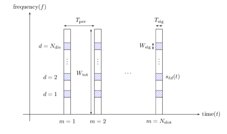
Figure 2: Periodic transmission of narrowband synchronization signals from the BS.

All the design options considered for initial access follow the same basic steps as shown in Figure 1. At a high level, these steps are identical to the methods used in 3GPP LTE, which are described in the specifications [29, 30, 31] as well as any standard text such as [32]. However, the depicted procedure needs major modifications for mmWave to enable both the UE and the BS to determine the initial BF directions in addition to detecting the presence of the BS and the access request from the UE. The steps are as follows. Note that since the most challenging task of mmWave IA is to determine the spatial signatures of the BS and the UE, we focus on the first two steps and do not elaborate on the rest.

1. Synchronization signal detection: Each cell periodically transmits synchronization signals that the UE can scan to detect the presence of the base station and obtain the downlink frame timing. In LTE, the first synchronization signal to detect is the Primary Synchronization Signal (PSS). For mmWave, the synchronization signal will also be used to determine the UE’s BF direction, which is related to the angles of arrival of the signal paths from the BS. Critical to our analysis, we will assume that the UE only attempts to learn the long-term BF directions [33], which depend only on the macro-level scattering paths and do not vary with small scale fading. The alternative, i.e., instantaneous beamforming, would require channel state information (CSI) at both TX and RX which may not be feasible at the initial stages of random access and also due to high Doppler frequencies, a point made in [8]. As a result, the long-term BF directions will be stable over much longer periods and thus will be assumed to be constant over the duration of the initial access procedure.

2. RA preamble transmission: Similar to LTE, we assume that the uplink contains dedicated slots exclusively for the purpose of random access (RA) messages. After detecting the synchronization signals and decoding the broadcast messages, the location of these RA slots is known to the UE. The UE randomly selects one of a small number (in LTE, there are up to 64) of waveforms, called RA preambles, and transmits the preamble in one of the RA slots. In all design options we consider below, the UE BF direction is known after step 0, so the RA preamble can be transmitted directionally, thereby obtaining the BF gain on the UE side. The BS will scan for the presence of the RA preamble and will also learn the BF direction at the BS side. As we discuss below, the method by which the BS will learn the BF direction will depend on the RA procedure.

3. Random access response (RAR): Upon detecting a RA preamble, the base station transmits a random access response to the UE indicating the index of the detected preamble. At this point, both the BS and the UE know the BF directions so all transmissions can obtain the full BF gain. The UE receiving the RAR knows its preamble was detected.

4. Connection request: After receiving RAR, the UE desiring initial access will send some sort of connection request message (akin to “Radio Resource Control (RRC) connection request” in LTE) on the resources scheduled in the uplink (UL) grant in the RAR.

5. Scheduled communication: At this point, all subsequent communication can occur on scheduled channels with the full BF gain on both sides.

Step	Item	Option	Explanation
0	Sync BS TX	Omni	BS transmits the downlink synchronization signal in a fixed, wide angle beam pattern to cover the entire cell area.
		Directional	BS transmits the downlink synchronization signal in time-varying narrow-beam directions to sequentially scan the angular space.
0	Sync UE RX	Directional	UE listens for the downlink synchronization signal in time-varying narrow-beam directions with analog BF that sequentially scans the angular space.
		Digital RX	UE has a fully digital RX and can thereby receive in all directions at once.
1	RA BS RX	Directional	In each random access slot, the BS listens for the uplink random access signal in time-varying narrow-beam directions using analog BF. The directions sequentially scan the angular space.
		Digital RX	The BS has a fully digital RX and can thereby receive in all directions in the random access slot at once.

TABLE I: Design options for each stage

II-B Synchronization and Random Access Signals

We assume that synchronization and random access signals are transmitted in relatively narrowband waveforms in periodically occurring intervals as shown in Figure  2. As shown in the figure, the synchronization signal is transmitted periodically once every $T_{\rm per,sync}$ seconds for a duration of $T_{\rm sig,sync}$ in each transmission. In LTE, the primary synchronization signal (PSS) is transmitted once every 5 ms for a duration of one OFDM symbol ($71.3~{}\mu$s). In this work, we will consider potentially different periods and signal lengths. We assume that the random access slots are located once every $T_{\rm per,RA}$ seconds and that the random access signals are of length $T_{\rm sig,RA}$. In LTE, the frequency of the random access slots is configurable and they are located at least once every 10 ms. Both the synchronization and the random access signals are assumed to be relatively narrowband with bandwidths $W_{\rm sig,sync}$ and $W_{\rm sig,RA}$, respectively. Note that in general, the periodicity, signal length, and signal bandwidth can be different for the synchronization and random access phases, resulting in different delays and overheads in the two cases. In this paper however, for the sake of simplicity and also to make the comparison between different design options more tractable, we take them to be equal for both phases and will refer to them simply as $T_{\rm per}$, $T_{\rm sig}$, and $W_{\rm sig}$, respectively.

Option	Sync BS TX	Sync UE RX	RA BS RX	$\bf{L}$		How the UE learns the BF direction	How the BS learns the BF direction
				Sync	RA
(a) DDO	Directional	Directional	Omni	$N_{\rm tx}N_{\rm rx}$	1	Directional scanning	The time slot index on which the UE received the sync signal is encoded in the RA preamble index (which reduces the number of available preamble waveforms). This way, the BS knows the TX direction in which the sync signal was received. Alternatively, the index of the time slot of the sync signal can be encoded implicitly in the RA preamble slot, which increases the access delay since the UE must wait for the appropriate access slot, but keeps all RA preamble waveforms available.
(b) DDD	Directional	Directional	Directional	$N_{\rm tx}N_{\rm rx}$	$N_{\rm tx}$	Same as (a)	Since the BS scans the directions for the RA preamble, the BF direction can be learned from the direction in which the RA preamble is received.
(c) ODD	Omni	Directional	Directional	$N_{\rm rx}$	$N_{\rm tx}$	Same as (a)	Same as option (b).
(d) ODDig	Omni	Directional	Digital RX	$N_{\rm rx}$	1	Same as (a)	With digital BF at the BS, the direction can be learned from the spatial signature of the received preamble.
(e) ODigDig	Omni	Digital RX	Digital RX	1	1	With digital BF at the UE, the direction can be learned from the spatial signature of the received sync signal	Same as option (d).

TABLE II: Design option combinations for initial access. The fifth and sixth columns are the size of the angular domain $L$ that has to be scanned for the Sync and the RA preamble detection respectively.

II-C Learning the BF Directions

While the basic procedure steps for initial access are similar to that used currently in LTE, the mmWave initial access procedure must include a method by which the base station and the UE can learn the directions of communication. The key modifications to enable this learning would occur in steps 0 and 1 of the procedure in Figure 1. In step 0, the UE must learn its BF direction, and in step 1 the BS learns the BF direction on its side. As stated earlier, these steps are the most challenging ones, hence we will focus on them. Table I shows some options for three items in this procedure, namely: (i) the manner in which the synchronization signal in step 0 is transmitted by the BS; (ii) the manner in which the synchronization signal is received at the UE; and (iii) the manner in which the random access preamble from the UE is received at the BS in step 1. For each item, we consider two possible options. For example, for the manner in which the synchronization signal is transmitted, we consider a fixed omni-directional transmission or a sequential scanning with directional transmissions. Note that since it is assumed that by the end of step 0 the UE has learned the correct direction of arrival from the BS , in step 1 it will always beamform in that direction to transmit the random access preamble.

Now, since there are two options for each of the three items in Table I, there are a total of eight design option combinations. However, for reasons that will become clear in the next section, we only consider five of these options. We will use the following nomenclature for these five options: They are named after the manner the Sync signal is transmitted (omni or analog directional) and how both the Sync and RA signals are received (analog directional or digital). For example, a design where the Sync signal is transmitted and received in analog directional while the RA preamble is received in the same manner is called DDD; and one where the signal is transmitted omni-directionally and received with digital BF in the Sync phase, and the RA preamble is received with digital BF is called ODigDig. We summarize the functionality and characteristics of these option combinations in Table II. This table includes the designs proposed in the recent works [34, 10].

II-D Sequential Beamspace Scanning

To analyze the different design options, we first need to quantify the time it takes to detect the synchronization and random access signals as a function of the SNR and signal overhead. We can analyze both the synchronization and RA phase with the same analysis. Suppose a transmitter (TX) repeatedly broadcasts some known signal once every $T_{\rm per}$ seconds as illustrated in Figure 2. For frequency diversity, we assume that each transmission consists of $N_{\rm div}$ subsignals transmitted in different frequency locations and that subsignals and their frequency locations are known to the receiver. The subsignals are assumed to be mostly constrained to some small time-frequency region of size $T_{\rm sig}\times W_{\rm sig}$. The goal of the receiver is to detect the presence of the signal, and, if it is present, detect its time and angle of arrival.

This model can be applied to analyze either the synchronization or the random access phase. In the synchronization phase (Step 0 of Figure 1), the TX will be the base station and the signal is the synchronization signal. In the random access phase (Step 1 of Figure 1), the TX will be the UE and the signal will be its random access preamble.

Now, for the moment, suppose that both the TX and the RX can perform only analog BF, so that they can only align their arrays in one direction at a time. We will address searching with hybrid and digital BF later – see Section III-B. To detect the synchronization signal, we assume that the TX and the RX cycle through $L$ possible TX-RX BF direction pairs. We will call each such cycle of $L$ transmissions a “directional scan” or “ scan cycle”. Since the transmission period is $T_{\rm per}$ seconds, each scan cycle will take $LT_{\rm per}$ seconds. We index the transmissions in each scan cycle by $\ell=1,\ldots,L$, and let $\mathbf{u}_{\ell}$ and $\mathbf{v}_{\ell}$ be the RX and TX beamforming vectors applied during the $\ell$-th transmission in each scan cycle. The same beamforming vectors are applied to all subsignals in each transmission.

There are a large number of options for selecting the $L$ direction pairs $(\mathbf{u}_{\ell},\mathbf{v}_{\ell})$ to use in each scan cycle – see, for example, [21] for a summary of some common methods. In this work, we will assume a simple beamspace sequential search. Given a linear or 2D planar array with $N$ antennas, the spatial signature of any plane wave on that array is given by the superposition of $N$ orthogonal directions called the beamspace directions. Each beamspace direction corresponds to a direction of arrival at a particular angle. In beamspace scanning, the TX and RX directions that need to be searched are selected from the orthogonal beamspace directions. If the TX and RX have $N_{\rm tx}$ and $N_{\rm rx}$ antennas, respectively, then the number $L$ of directions to scan is given by:

• $L=N_{\rm tx}N_{\rm rx}$ if both the TX and RX scan over all the beamspace directions;

• $L=N_{\rm tx}$ if only the TX scans while the RX uses an omni-directional or fixed antenna pattern;

• $L=N_{\rm rx}$ if only the RX scans while the TX uses an omni-directional or fixed antenna pattern;

• $L=1$ if both the TX and RX use omni-directional (or fixed antenna patterns) or digital BF. In the latter case, unlike in analog BF the digital receiver can “look” into all $N_{\rm rx}$ directions simultaneously while maintaining the RX directivity gain.

The TX and RX continue repeating the transmission scans until either the signal is detected or the procedure times out. Therefore, the size of the angular space $L$ is directly connected to the delay of signal detection since more time is needed to cover all the angular pairs as $L$ grows. In Table II, for each design we have put the respective number of directions $L$ in both Sync and RA. Note that RA’s $L$ is always less than or equal to Sync’s $L$ since after step 0, the position of the BS is assumed to be known and only one side may need to scan the angular space.

In Section II-C we mentioned that we present only five designs out of the eight possible combinations of Table I. The explanation is that every one of the three designs omitted share the same number of directions to scan $L$ with some of the five basic designs and their performance in delay was assessed to be no different than the ones presented in Table II.

III Signal Detection under a Sequential Beamspace Scanning

III-A Generalized likelihood ratio (GLRT) Detection

Given the above transmissions, the RX must determine whether the signal is present, and, if it is present, determine the direction of maximum energy. To make this decision, suppose that the RX listens to $K$ scan cycles for a total of $LK$ transmissions. Index the transmissions within each scan cycle by $\ell=1,\ldots,L$ and the cycles themselves by $k=1,\ldots,K$. We assume that each transmission occurs in some signal space with $M$ orthogonal degrees of freedom and we let $\mathbf{s}_{\ell d}\in{\mathbb{C}}^{M}$ be the signal space representation of the $d$-th subsignal transmitted in the $\ell$-th transmission in each scan cycle where $d=1,\ldots,N_{\rm div}$. If the subsignal can be localized to a time interval of length $T_{\rm sig}$ and bandwidth $W_{\rm sig}$, then the number of degrees of freedom is approximately $M\approx T_{\rm sig}W_{\rm sig}$.

We assume that in the $\ell$-th transmission within each scan cycle, the RX and TX apply the beamforming vectors $\mathbf{u}_{\ell}\in{\mathbb{C}}^{N_{\rm rx}}$ and $\mathbf{v}_{\ell}\in{\mathbb{C}}^{N_{\rm tx}}$. We assume that the received complex baseband signal in the $d$-th subsignal in the $\ell$-th transmission and $k$-th scan cycle can be modeled as

$$\mathbf{r}_{k\ell d}=\mathbf{u}^{*}_{\ell}\mathbf{H}_{k\ell d}\mathbf{v}_{\ell}\mathbf{s}_{\ell d}+\mathbf{w}_{k\ell d},\quad\mathbf{w}_{k\ell d}\sim{\mathcal{N}}(0,\tau_{k\ell d}\mathbf{I}_{M}),$$ (1)

where $\mathbf{r}_{k\ell d}\in{\mathbb{C}}^{M}$ is the signal space representation of the received subsignal after beamforming; $\mathbf{H}_{k\ell d}$ is the complex MIMO fading channel matrix during the transmission, and $\mathbf{w}_{k\ell d}$ is complex white Gaussian noise (WGN) with some variance $\tau_{k\ell d}$ in each dimension. We have assumed that the signal in each transmission is transmitted in a sufficiently small time and frequency bandwidth so that the channel can be approximated as constant and flat within that transmission.

Our first key simplifying assumption is that the true channel between the TX and RX, if it exists, is described by a single LOS path exactly aligned with one of the $L$ TX-RX beamspace directions. That is,

$$\mathbf{H}_{k\ell d}=h_{k\ell d}\mathbf{u}_{\ell_{0}}\mathbf{v}_{\ell_{0}}^{*},$$ (2)

so that the channel’s TX direction $\mathbf{v}_{\ell_{0}}$ and RX direction $\mathbf{u}_{\ell_{0}}$ are each aligned exactly along one of the TX and RX beamspace directions, $\mathbf{v}_{\ell}$ and $\mathbf{u}_{\ell}$. The coefficient $h_{k\ell d}$ is a scalar small-scale fading coefficient that may vary with the subsignal $d$, transmission $\ell$ and scan cycle $k$. Of course, real channels are composed of multiple path clusters with beamspread, none of which will align exactly with one of the directions. However, we will use this idealized beamspace model only to simplify the detector design and analysis. Our simulations, on the other hand, will be performed using a measurement-based realistic channel model.

Now, if we assume that the beamforming directions are orthonormal, i.e., $\mathbf{u}_{\ell}^{*}\mathbf{u}_{\ell_{0}}\mathbf{v}_{\ell}^{*}\mathbf{v}_{\ell_{0}}=\delta_{\ell,\ell_{0}},$ we can rewrite (1) as

$$\mathbf{r}_{k\ell d}=\psi_{kd}\delta_{\ell,\ell_{0}}\mathbf{s}_{\ell d}+\mathbf{w}_{k\ell d},$$ (3)

where $\psi_{kd}=h_{k\ell_{0}d}$ and $\ell_{0}$ is the true direction. The variable $\psi_{kd}$ is the complex gain on the $d$-th subsignal in the $k$-th scan cycle at the time when the beam directions are properly aligned.

The detection problem can then be posed as a hypothesis testing problem. Specifically, the presence or absence of the signal corresponds to two hypotheses:

$$\begin{array}[]{ll}H_{0}:~{}\psi_{kd}=0&\mbox{(signal absent),}\\ H_{1}:~{}\psi_{kd}\neq 0&\mbox{(signal present).}\end{array}$$ (4)

Now, the model in (3) specifies the probability distribution of the observed data, which we denote as

$$p(\mathbf{r}|{\bm{\tau}},{\bm{\psi}},\ell_{0}),$$ (5)

where $\mathbf{r}=\{\mathbf{r}_{k\ell d}\}$ is the set of all measurements, ${\bm{\tau}}=\{\tau_{k\ell d}\}$ is the set of noise levels, ${\bm{\psi}}=\{\psi_{kd}\}$ is the set of signal levels. Since the model has unknown parameters, we follow the procedure in [14] and use a standard Generalized Likelihood Ratio Test (GLRT) [35] to decide between the two hypothesis. Specifically, we first compute the minimum negative log likelihood (ML) of each hypothesis,

$$\Lambda_{0}:=\min_{{\bm{\tau}},\ell_{0}}-\ln p(\mathbf{r}|{\bm{\tau}},{\bm{\psi}}=0,\ell_{0})$$ (6a)

$$\Lambda_{1}:=\min_{{\bm{\tau}},{\bm{\psi}},\ell_{0}}-\ln p(\mathbf{r}|{\bm{\tau}},{\bm{\psi}},\ell_{0}),$$ (6b)

and then use the test

$$\widehat{H}=\begin{cases}1&\Lambda_{0}-\Lambda_{1}\geq t\\ 0&\Lambda_{0}-\Lambda_{1}<t,\end{cases}$$ (7)

where $t$ is a threshold. It is shown in Appendix A that the test can be computed as follows. For each transmission $\ell$ in scan cycle $k$, we compute the correlation

$$\rho_{k\ell d}:=\frac{|\mathbf{s}_{\ell d}^{*}\mathbf{r}_{k\ell d}|^{2}}{\|\mathbf{s}_{\ell d}\|^{2}\|\mathbf{r}_{k\ell d}\|^{2}}.$$ (8)

This is simply a matched filter. We next compute the optimal beamspace direction by minimizing

$$\widehat{\ell}_{0}=\mathop{\mathrm{arg\,min}}_{\ell=1,\ldots,L}\sum_{k=1}^{K}\sum_{d=1}^{N_{\rm div}}\ln\left(1-\rho_{k\ell d}\right).$$ (9)

Then, it is shown in Appendix A that the log likelihood difference is given by

$$\Lambda_{0}-\Lambda_{1}=M\sum_{k=1}^{K}\sum_{d=1}^{N_{\rm div}}\ln\left(1-\rho_{k\widehat{\ell}_{0}d}\right),$$ (10)

which can be applied into the hypothesis test (7).

III-B Hybrid and Digital Beamforming

The above detector was derived for the case of analog BF. However, the same detector can be used for hybrid and digital BF. In hybrid BF at the RX, the RX has $S$ complete RF chains and thus has the ability to operate as $S$ analog BF systems in parallel. Thus, an identical detector can be used. The only difference is that one can obtain $S$ power measurements in each time instant – hence speeding up the detection by a factor of $S$.

For digital BF, one can simply test all $N_{\rm rx}$ directions in each time step, which is again equivalent to analog BF but with an even faster acceleration. Note that in digital BF, one can also test angles of arrival that are not exactly along one of the $N_{\rm rx}$ beamspace directions. However, to keep the analysis of various design options simple we will not consider this detector but assume that in digital BF the arrival angles are aligned with the beamspace directions.

Of course, as discussed above, digital BF may require much higher power consumption to support separate ADCs for each antenna element. In the analysis below, we will thus consider a low-resolution digital architecture.

IV Delay Analysis

Given the search algorithm, we can now evaluate each of the design options described in Table II. Our goal is to determine two key delay parameters: (1) The synchronization delay, i.e., the time it takes the UE to detect the presence of the synchronization signal in Step 0 of Figure 1, and (2) the RA preamble detection delay, i.e., the time the BS needs to reliably detect the random access preamble in Step 1. These first two steps will be the dominant components of the overall delay for initial access. We call the sum of the synchronization and RA delay the access delay. Note that this delay is the baseline for the total, control plus data plane, latency. Due to beam “fine-tuning” and channel estimation delay before each transmission in data plane, a subject discussed in [36] and [37], it is crucial to push the access delay as low as possible in order to achieve the very high throughput and low latency targets set for 5G [5].

Before undertaking a detailed numerical simulation, it is useful to perform a simple theoretical analysis that illustrates the fundamental relations between beamforming gains and delay for the different design options. We focus on the synchronization phase which, since both the UE and the BS don’t know the correct directions, is more challenging than RA. To this end, suppose the initial access system targets all UEs whose SNR is above some minimum target value, $\gamma_{\rm tgt}$. This target SNR may be defined for a target rate the UE is assumed to require when in connected mode, and should be measured relative to the SNR that a UE could get with beamforming gains, i.e.,

$$\gamma_{\rm tgt}=\frac{PG_{\rm rx}G_{\rm tx}}{N_{0}W_{\rm tot}},$$ (11)

where $P$ is the omni-directional received power (affected by the pathloss), $W_{\rm tot}$ the total available bandwidth in connected mode, and $G_{\rm rx}$ and $G_{\rm tx}$ are the maximum RX and TX antenna gains, i.e., the gains that the link could enjoy if the directions were perfectly aligned.

Now, let $\gamma_{\rm sig}$ be the minimum SNR accumulated on the synchronization signal required for reliable detection (the precise value will depend on the false alarm and misdetection probabilities). Each synchronization transmission will have an omni-directional received energy of $PT_{\rm sig}$. In all design options in the synchronization phase, the UE scans the space directionally, obtaining a maximum gain of $G_{\rm rx}$ when the beams are aligned. We let $G_{\rm tx}^{\rm sync}$ be the maximum TX beamforming gain available in the synchronization phase: $G_{\rm tx}^{\rm sync}=1$ for the omni-directional transmission and $G_{\rm tx}^{\rm sync}=G_{\rm tx}$ for the case of directional transmissions. Thus, when the beams are correctly aligned, the synchronization signal will have a received energy of $G_{\rm rx}G_{\rm tx}^{\rm sync}PT_{\rm sig}.$ The beams will be correctly aligned exactly once every scan cycle, and hence, to obtain reliable detection after $K$ scan cycles we need

$$\frac{KPT_{\rm sig,sync}G_{\rm rx}G_{\rm tx}^{\rm sync}}{N_{0}}\geq\gamma_{\rm sig}.$$ (12)

Following Fig. 2, the synchronization signal occupies $T_{\rm sig,sync}$ seconds every $T_{\rm per,sync}$ seconds and hence the overhead is

$$\phi_{\rm ov,sync}=T_{\rm sig,sync}/T_{\rm per,sync},$$ (13)

and the time to perform $K$ scan cycles in

$$D_{\rm sync}=KLT_{\rm per,sync}.$$ (14)

Combining (11), (12) and (13), the synchronization delay $D_{\rm sync}$ can be bounded as

$$D_{\rm sync} =KLT_{\rm per,sync}\geq\frac{\gamma_{\rm sig}LG_{\rm tx}}{G_{\rm tx}^{\rm sync}\gamma_{\rm tgt}W_{\rm tot}\phi_{\rm ov,sync}}.$$ (15)

Now, the antenna gain is proportional to the number of antennas, and we will thus assume that the maximum gain is given by $G_{\rm rx}=N_{\rm rx},\quad G_{\rm tx}=N_{\rm tx}.$ Also, for the analog BF options, ODx and DDx, it can be verified that $L=G_{\rm rx}G_{\rm tx}^{\rm sync}$, so

$$D_{\rm sync}\geq\frac{\gamma_{\rm sig}G_{\rm rx}G_{\rm tx}}{\gamma_{\rm tgt}W_{\rm tot}\phi_{\rm ov,sync}}.$$ (16)

This bound may not be achievable, since it may require that the synchronization signal duration $T_{\rm sig,sync}$ is very small. Very short synchronization signals may not be practical since the signal needs sufficient degrees of freedom to accurately estimate the noise in addition to the signal power – we will see this effect in the numerical simulations below. Thus, suppose there is some minimum practical synchronization signal time, $T_{\rm sig,sync}^{\rm min}$. Since $K\geq 1$,

$$D_{\rm sync} =KLT_{\rm per}\geq\frac{LT_{\rm sig,sync}}{\phi_{\rm ov,sync}}$$

$$\geq\frac{LT_{\rm sig,sync}^{\rm min}}{\phi_{\rm ov,sync}}=\frac{G_{\rm rx}G_{\rm tx}^{\rm sync}T_{\rm sig,sync}^{\rm min}}{\phi_{\rm ov,sync}},$$ (17)

Combining (16) and (17),

$$D_{\rm sync}\geq\frac{G_{\rm rx}}{\phi_{\rm ov,sync}}\max\left\{\frac{\gamma_{\rm sig}G_{\rm tx}}{\gamma_{\rm tgt}W_{\rm tot}},G_{\rm tx}^{\rm sync}T_{\rm sig,sync}^{\rm min}\right\}.$$ (18)

The digital case is similar except that $L=G_{\rm tx}^{\rm sync}$ since only the transmitter needs to sweep the different directions. Hence, the synchronization delay is reduced by a factor of $G_{\rm rx}$:

$$D_{\rm sync}\geq\frac{1}{\phi_{ov,sync}}\max\left\{\frac{\gamma_{\rm sig}G_{\rm tx}}{\gamma_{\rm tgt}W_{\rm tot}},G_{\rm tx}^{\rm sync}T_{\rm sig,sync}^{\rm min}\right\}.$$ (19)

This simple analysis reveals several important features. First consider the delay under analog BF in (18). Without a bound on $T_{\rm sig,sync}$, both analog BF options ODx and DDx will have the same delay, and the delay grows linearly with the combined gain $G_{\rm rx}G_{\rm tx}$. Hence, there is a direct relation between delay and the amount of BF gain used in the system. However, when using a signal duration equal to the bound $T_{\rm sig,sync}^{\rm min}$, the second term in the maximum in (18) will become dominant. In this case, an omni directional transmission will have a lower bound delay of only $T_{\rm sig,sync}^{\rm min}$ (since $G^{\rm sync}_{\rm tx}=1$), while a directional one will be lower-bounded by $G^{\rm sync}_{\rm tx}T_{\rm sig,sync}^{\rm min}>T_{\rm sig,sync}^{\rm min}$.

Finally, digital BF at the UE (Option DDigX) offers a significant improvement over both analog options by a factor of $G_{\rm rx}$. Hence, in circumstances where the UE has a high directional gain antenna, the benefits can be significant.

V Numerical Evaluation

V-A System Parameters

The above analysis is highly simplified and, while useful to gain some intuition and basic understanding, cannot be used to make detailed system design choices. For a more accurate analysis of the delay, we assessed the delay under realistic system parameters and channel models. Appendix B provides a detailed discussion on the reasoning behind the parameter selection. In brief, the signal parameters $T_{\rm sig}$ and $W_{\rm sig}$ were selected to ensure that the channel is roughly flat within each $T_{\rm sig}\times W_{\rm sig}$ subsignal time-frequency region based on the typical values of the coherence time and the coherence bandwidth observed in [38, 39]. The parameter $T_{\rm sig}$ was also selected sufficiently short so that the Doppler shift across the subsignal would not be significant with moderate UE velocities (30 km/h). Depending on the overhead that we can tolerate for synchronization and random access signals, different values for $T_{\rm per}$ are selected. The use of $N_{\rm div}=4$ subsignals was found experimentally to give the best performance in terms of frequency diversity versus energy loss from non-coherent combining. For the antenna arrays, we followed the capacity analysis in [8] and considered 2D uniform planar arrays with $4\times 4$ elements at the UE, and $8\times 8$ at the BS.

To compute the threshold level $t$ in (10), we first computed a false alarm probability target with the formula

$$P_{\textsc{F}A}=\frac{R_{\textsc{F}A}}{N_{\rm sig}N_{\rm dly}N_{\textsc{F}O}},$$

where $R_{\textsc{F}A}$ is the maximum false alarm rate per search period over all signal, delay and frequency offset hypotheses and $N_{\rm sig}$, $N_{\rm dly}$ and $N_{\textsc{F}O}$ are, respectively, the number of signal, delay and frequency offset hypotheses. Again, the details of the selection are given in Appendix B. $N_{\rm dly}$ represents the number of delay hypotheses in each transmission period in either uplink or downlink. The detector has to decide at which delay $\tau$ the signal was received. The granularity of searching for the correct $\tau$ is at the level of one out of all the samples between two transmission periods $T_{\rm per}$. Assuming sampling at twice the bandwidth, in the downlink direction, this is $\frac{1}{2W_{\rm sig,sync}\times T_{\rm per,sync}}$. Hence, the number of delay hypotheses, $N_{\rm dly}$, is equal to all these possible $\tau$s. In other words, $N_{\rm dly}=2W_{\rm sig,sync}T_{\rm per,sync}$. Note that, since the signal is transmitted periodically, $N_{\rm dly}$ stays constant and does not increase as time passes. In the uplink direction we have $N_{\rm dly}=2W_{\rm sig,RA}T_{\rm offset}$, where $T_{\rm offset}$ is the round trip time of the signal propagation between UE and BS (See Appendix B for why this number is different for RA and Sync.) The number of frequency offset hypotheses $N_{\textsc{F}O}$ was computed so that the frequency search could cover both an initial local oscillator (LO) error of $\pm 1$ part per million (ppm) as well as a Doppler shift up to 30 km/h at 28 GHz. We selected $N_{\rm sig}=3$ for the number of signal hypotheses in the synchronization step and $N_{\rm sig}=64$ for the random access step as used in current 3GPP LTE. We then used a large number of Monte Carlo trials to find the threshold to meet the false alarm rate. Having set this target $P_{FA}$, we essentially wish to find the correlation $\rho_{k\ell d}$ at point $t$ which corresponds to this probability. This point will be the detection threshold [35]. As long as $\rho_{k\ell d}$ is below this threshold the detector assumes that just noise is being received, while if $\rho_{k\ell d}$ goes above it, the detector will assume $\rho_{k\ell d}=\rho_{k\hat{\ell}_{0}d}$ and hence an estimate of the correct angle $\ell_{0}$ is found. As shown in Appendix B for our selected parameters, $P_{\textsc{F}A}$ becomes very small. Therefore, we extrapolated the tail distribution of the statistic $T=\rho_{k\ell d}$ of the test defined by (7) and (10), to estimate the threshold analytically. To this end we used a second degree polynomial fit for $\log\Pr(T>t)$ [14].

Parameter	Value
Total system bandwidth, $W_{\rm tot}$	1 GHz
Number of subsignals per time slot, $N_{\rm div}$	$4$
Subsignal Duration, $T_{\rm sig}$	varied ($10$ $\mu$s, $50$ $\mu$s, $100$ $\mu$s)
Subsignal Bandwidth, $W_{\rm sig}$	1 MHz
Period between transmissions, $T_{\rm per}$	Varied to meet overhead requirements
Total false alarm rate per scan cycle, $R_{\textsc{F}A}$	$0.01$
Number of sync signal waveform hypotheses	$3$
Number of RA preambles	$64$
Number of frequency offset hypotheses, $N_{\textsc{F}O}$	$23$
BS antenna	$8\times 8$ uniform planar array
UE antenna	$4\times 4$ uniform planar array
Carrier Frequency	28 GHz
Cell radius	100 m
Number of bits in the low resolution digital architecture	3 per I/Q

TABLE III: Default simulation parameters unless otherwise stated.

Parameter	Value
Cell radius, $r$	$100$ m
Downlink TX power	$30$ dBm
Uplink TX power	$20$ dBm
BS noise figure, $NF_{BS}$	$4$ dB
UE noise figure, $NF_{UE}$	$7$ dB
Thermal noise power density, $kT$	$-174$ dBm/Hz
Carrier Frequency	28 GHz
Total system bandwidth, $W_{\rm tot}$	1 GHz
Probability of LOS vs. NLOS	$P_{LOS}(d)=\exp(-a_{los}d)$, $a_{los}=67.1$ m
Path loss model dB	$PL(d)=\alpha+10\beta\log 10(d)+\xi$ $\xi\sim\mathcal{N}(0,\sigma^{2})$, $d$ is in meters
NLOS parameters	$\alpha=72.0$, $\beta=2.92$, $\sigma=8.7$ dB
LOS parameters	$\alpha=61.4$, $\beta=2.0$, $\sigma=5.8$ dB

TABLE IV: SNR simulation parameters.

V-B SNR

We used the following model for the SNR distribution. We envision a cell area of radius $r=100$ m with the mmWave BS at its center, and UEs randomly “dropped” within this area. We then compute a random path loss between the BS and the UEs based on the model in [8]. This model was obtained from data gathered in multiple measurement campaigns in downtown New York City [38, 40, 41, 3, 39]. The path loss model parameters, along with the rest of the simulation parameters, are given in Table IV.

In the model in [8], the channel/link between a UE and a BS is randomly selected, according to some distance dependent probabilities, to be in one of three states, namely, LOS, NLOS or outage. Here, we ignore the outage state, since UEs in outage cannot establish a link, and instead focus on the other two states, in which initial access can be performed. A UE may be in either state with probabilities $P_{\textsc{L}OS}(d)$ or $P_{\textsc{N}LOS}=1-P_{\textsc{L}OS}(d)$. The omni-directional path loss is then computed from

$$PL=\alpha+10\beta\log 10(d)+\xi\;[dB],\;\xi\sim\mathcal{N}(0,\sigma^{2}),$$

where the parameters $\alpha$, $\beta$ and $\sigma$ depend on the LOS or NLOS condition and $d$ is the distance between the transmitter and the receiver.

We do not consider interference from other cells. In the downlink, since the bandwidth in mmWave cells is large, we assume that neighboring cells can be time synchronized and place their synchronization signals on non-overlapping frequencies. Since we assume that there are no other signals transmitted during the synchronization signal slot (see Fig. 2), using partial frequency reuse does not increase the overhead. In the uplink, we ignore collisions from other random access transmissions either in-cell or out-of-cell, so again we can ignore the interference.

Fig. 3 shows the DL and UL SNR distributions under these assumptions. The SNR plotted is measured on a total bandwidth of $W_{\rm tot}=1$ GHz,

$$\mbox{\small SNR}_{\rm data,omni}=\frac{P}{N_{0}W_{\rm tot}},$$ (20)

where $P$ is the received power and $N_{0}$ is the noise power spectral density (including the noise figure). Note that this is the omni-directional SNR and hence does not include the beamforming gain.

The synchronization and RA signals are transmitted in much narrower bands and therefore will have higher SNRs in the signal bandwidth. The reason we plot the SNR with respect to the total bandwidth is that we believe it makes it easier to interpret the results of Fig. 3. Plotting the narrowband RA/Sync SNRs would be somehow irrelevant since they are meaningless beyond the context of these very signals. It is the SNR over the whole available bandwidth $W_{\rm tot}$ that defines the SNR regime where a UE operates. It is this SNR that determines the data rates in both DL and UL – See Appendix B for the connection between $\mbox{\small SNR}_{\rm data,omni}$ and the signals’ SNRs. Also plotted are the $1\%$ and $5\%$ percentiles and the median lines for the UL and DL.

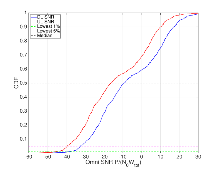
Figure 3: SNR distribution in downlink and uplink for a cell of radius 100 m.

V-C Fully Digital BF with Low Bit Resolution

Two of the options in Table II require fully digital receivers: ODDig requires a fully digital front-end at the BS and ODigDig requires one at both the UE and the BS. Deploying such a fully digital front end comes at the potential cost of high power consumption due to the need for one analog to digital converter (ADC) per antenna element. This problem is especially of concern on the UE side where the power consumption of the device should remain as low as possible.

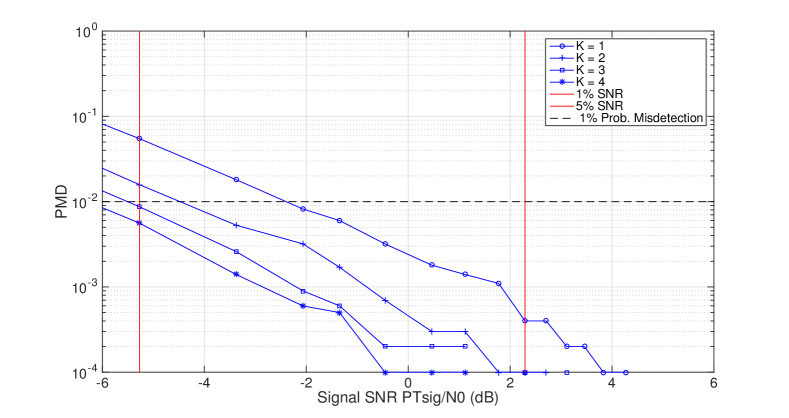
Figure 4: DDD/DDO, probability of misdetection (PMD) versus synchronization signal SNR for $K=1,2,3,4$. Each additional cycle decreases the misdetection probability for a given SNR regime.

To properly compare fully digital options with the analog BF cases, we constrain the digital architecture to have the power consumption in the same order as the analog BF case by using a very small number of bits per I/Q dimension. Such low bit resolution mmWave front-ends have been studied in [22, 23, 42, 43, 44]. In [44] specifically, the authors discuss among other things the impact of ADC resolution on the communication rate after the link has been established. The concept is that the power consumption of an ADC generally scales as $2^{b}$, where $b$ is the number of bits  [45]. In the analysis below, we will constrain the fully digital architecture to have $b=3$ bits per I/Q dimension at most. Since conventional ADCs typically have near 10 bits, using 3 bits should reduce the power consumption by a factor of 128 which more than compensates for adding an ADC on all 16 or 64 elements of the antenna array.

Number bits	Quantization loss, $-10\log_{10}\frac{\gamma_{\rm hq}}{\gamma_{\rm lq}}$ (dB)
1	1.96
2	0.54
3	0.15

TABLE V: Quantization loss as a function of the number of bits for a scalar uniform quantizer with Gaussian noise.

To analyze the effect of the low resolution, we use a standard additive noise quantization model [46, 47] as used in the analysis of fully digital receivers for cell search in [14]. There it is shown that the effective SNR due to the quantization noise is given by

$$\gamma_{\rm lq}=\frac{(1-\sigma)\gamma_{\rm hq}}{1+\sigma\gamma_{\rm hq}},$$ (21)

where $\gamma_{\rm lq}$ and $\gamma_{\rm hq}$ are the effective SNR of the low resolution ADC, and the initial SNR of the high resolution ADC, respectively. The factor $\sigma$ is the average relative error of the quantizer and depends on the quantizer design, input distribution and number of bits. Equation (21) shows that at very low SNRs, the quantization results in a loss of $1-\sigma$. Table V shows this loss for $b=1$ to 3 bits using the numbers from [14]. We see that at $b=3$, the quantization loss is only 0.15 dB. In all the subsequent analysis below, we will restrict the digital solutions to have only $b=3$ bits and use (21) to transform the SNRs to account for the increased quantization noise.

Option	$T_{\rm sig}$	$L$		1% SNR				5% SNR				High SNR
		Sync	RA	Sync		RA		Sync		RA		Sync		RA
				$K^{*}$	delay	$K^{*}$	delay	$K^{*}$	delay	$K^{*}$	delay	$K^{*}$	delay	$K^{*}$	delay
DDO	$10~{}\mu$s			3	614.4	2393	478.6	1	204.8	65	13	1	204.8	1	0.2
	$50~{}\mu$s	1024	1	1	1024	60	60	1	1024	3	3	1	1024	1	1
	$100~{}\mu$s			1	2048	17	34	1	2048	2	4	1	2048	1	2
DDD	$10~{}\mu$s			3	614.4	24	307.2	1	204.8	2	25.6	1	204.8	1	12.8
	$50~{}\mu$s	1024	64	1	1024	2	128	1	1024	1	64	1	1024	1	64
	$100~{}\mu$s			1	2048	1	128	1	2048	1	128	1	2048	1	128
ODD	$10~{}\mu$s			73	233.6	24	307.2	4	12.8	2	25.6	1	3.2	1	12.8
	$50~{}\mu$s	16	64	3	48	2	128	1	16	1	64	1	16	1	64
	$100~{}\mu$s			1	32	1	128	1	32	1	128	1	32	1	128
ODDig	$10~{}\mu$s			73	233.6	25	5	4	12.8	2	0.4	1	3.2	1	0.2
	$50~{}\mu$s	16	1	3	48	2	2	1	16	1	1	1	16	1	1
	$100~{}\mu$s			1	32	1	2	1	32	1	2	1	32	1	2
ODigDig	$10~{}\mu$s			79	15.8	25	5	4	0.8	2	0.4	1	0.2	1	0.2
	$50~{}\mu$s	1	1	4	4	2	2	1	1	1	1	1	1	1	1
	$100~{}\mu$s			2	4	1	2	1	2	1	2	1	2	1	2

TABLE VI: Detection delays in milliseconds for a fixed overhead of 5$\%$. The third and fourth column show the size of the angular space $L$ that has to be scanned in Sync and RA for each option. Note that they are the same as the fifth and sixth columns of Table III except that we have assigned numbers to $N_{\rm tx}$ and $N_{\rm rx}$. $K^{*}$ is the number of full cycles required for detection in each scenario. Values for digital BF are derived given an ADC with 3 bit resolution.

V-D Multipath NYC Channel Model

In deriving the GLRT detector in Section III-A we assumed that the channel gain was concentrated in a single path aligned exactly with one of the $L$ beamspace direction pairs. This assumption may look naive at first, since real channel measurements have shown that the mmWave channel exhibits multipath characteristics [38, 40, 41, 3, 39]. However, the fundamental difficulty in Sync/RA signal detection arises from the potentially large size of the angular space and the time needed to cover it. Our detector sufficiently captures this difficulty for each and every one of the presented designs. Moreover, in our previous work [14], we showed that a multipath channel helps in detecting the desired signal as it provides more discovery opportunities through multiple macro-level scattering paths. Nevertheless, while we will use this detector, we simulate and evaluate our proposed designs against a realistic spatial non-line of sight (NLOS) channel model in [8] derived from actual 28 GHz measurements in New York City [38, 40, 41, 3, 39]. Due to limited space, we do not provide a detailed discussion on this channel model here, and just mention that it is described by multiple random clusters, with random azimuth and elevation angles and beamspread – see [8] for details. Finally, we note that the proposed analysis and methodology are general and, although used here in combination with the NYU measurement-based channel model to evaluate and compare the design options, can be applied to any other channel model or measurement data set.

V-E Synchronization Delay

We now proceed to evaluate the delays for each of the proposed options in Table II. We first estimate the number of scan cycles $K$ it takes to reliably detect the synchronization signal from the BS. This depends on the design option and the SNR. Figure 4 shows the probability of misdetection ($P_{MD}$) as a function of the SNR and of the number of scan cycles $K$ for the DDD/DDO design options, evaluated via on Monte Carlo simulations. Recall that the false alarm rate was set to $R_{\textsc{F}A}=0.01$ per scan cycle. Also plotted are the vertical lines for the lowest $1\%$ and $5\%$ of the SNR DL distributions described in Section V-B. We set a target misdetection rate of $P_{MD}=0.01$ for a Sync signal of duration $T_{\rm sig,sync}=10$ $\mu$s. We observe in the same figure that the 1% cell edge users, as defined by the SNR distribution obtained in Section V-B, will require $K=3$ scan cycles to meet the target while the 5% and above users (according to the same distribution) are able to pass the detection target in just one scan cycle.

The simulation is repeated for the other design options and different values of $T_{\rm sig,sync}$. Based on the minimum number of required scan cycles, we can then compute the synchronization delay as a function of the overhead. Following the analysis of Section IV, the relation between delay and overhead is $D_{\rm sync}=KLT_{\rm per,sync}=\frac{KLT_{\rm sig,sync}}{\phi_{\rm ov,sync}}.$ Using $K$ from the simulation, Table VI shows the delays $D_{\rm sync}$ for a fixed overhead of $\phi_{\rm ov,sync}=$ 5%.

The minimum synchronization signal time we consider is $T_{\rm sig,sync}^{min}=10~{}\mu$s. Since each synchronization subsignal is transmitted over a narrow band $W_{\rm sig}$, the degrees of freedom in each subsignal are $T_{\rm sig}W_{\rm sig}$. Since we have assumed $W_{\rm sig}=1$ MHz, using $T_{\rm sig,sync}=10~{}\mu$s would provide 10 degrees of freedom, and thus 9 degrees of freedom on which to estimate the noise variance.

In Figure 5, the synchronization delay is illustrated as a function of the overhead.

There are two important results: First, for analog BF, the omni-directional transmissions (options ODx) outperform directional transmissions (Option DDx). This is consistent with the analysis in Section IV: since the directional transmissions were using the minimum $T_{\rm sig}$, the omni-directional transmissions provided a benefit (see the second part of the max in (18)). Second, we see that digital reception (Option ODigDig) in both SNR regimes significantly outperforms other schemes for all overhead ratios. The digital BF curve accounts for the fact that we are using low-resolution quantization to keep the power consumption roughly constant. The gain with digital BF is due to its ability to “look” into multiple directions at once while exploiting directionality at both RX and TX, and is clearly observable when comparing the high SNR curves of DDO and ODigDig, as predicted by (19).

V-F Random Access Delay

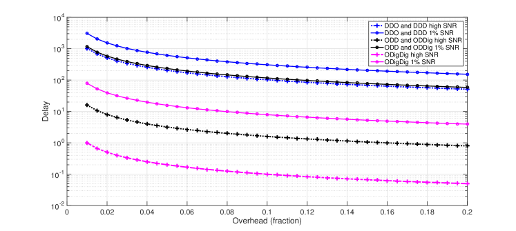
Figure 5: Synchronization delay in ms versus signal overhead for the minimum Sync signal duration $T_{\rm sig,sync}^{\rm min}=10$ ${\rm\mu}$s.

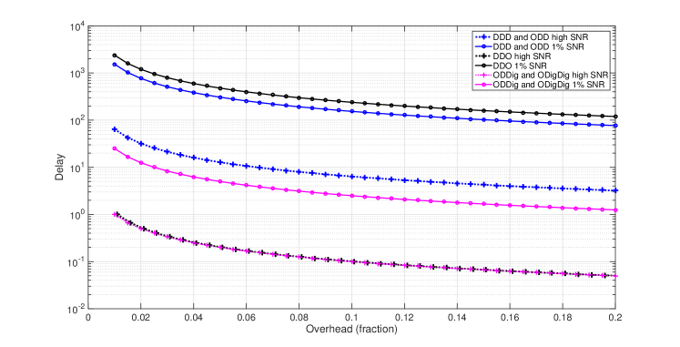
Figure 6: Synchronization delay in ms versus signal overhead for the minimum Sync signal duration $T_{\rm sig,RA}^{min}=10$ ${\rm\mu}$s.

For the Random access phase, we perform a detection procedure similar to that of synchronization. We consider the same SNR regimes for edge and high SNR users as before, and we can compute the RA overhead as

$$\phi_{\rm ov,\textsc{R}A}=T_{\rm sig,\textsc{R}A}/T_{\rm per,\textsc{R}A}.$$ (22)

It should be noted that in digital BF or hybrid BF with more than one stream, a lower overhead may be possible: With digital or multi-stream hybrid BF, in the same time slot of any RA period, a BS can theoretically schedule uplink transmissions from UEs that are already connected. This is not possible with analog BF with one stream since the BS in that case can only “look” in one direction at a time. Since the RA signals occupy a total frequency of $N_{\rm div}W_{\rm sig,\textsc{R}A}$, the total overhead with digital BF or multi-stream hybrid BF is

$$\phi_{\rm ov,\textsc{R}A}=W_{\rm sig,\textsc{R}A}T_{\rm sig,\textsc{R}A}/(W_{\rm tot}T_{\rm per,\textsc{R}A}).$$ (23)

Since this multiplexing would require a potentially larger dynamic range, possibly not afforded by low-resolution ADCs, the analysis below will forgo this potential improvement until further investigation can be conducted. In the meantime, we will conservatively assume that the overhead in (22) applies to both digital and analog BF. The detection delay is then given by $D_{\rm RA}=KLT_{\rm per,RA}=\frac{KLT_{\rm sig,RA}}{\phi_{\rm ov,RA}}.$

Also, the same minimum duration $T_{\rm sig,RA}^{min}=10~{}\mu$s is considered. What is inherently different in RA, compared to the synchronization phase, is that the beam space is always smaller. This is due to the fact that RA follows the synchronization phase. Therefore, the UE has already obtained the correct angle to the BS and transmits its RA preamble only in that direction. Also, the number of the delay hypotheses is considerably smaller and is a function of the propagation round trip time. This is because we can assume that by detecting the synchronization signal, the UE learns where in the frame the BS expects the RA requests - see Appendix B.

Figure 6 and Table VI summarize the results of our RA simulations. As in synchronization, to achieve both low overhead and delay, digital RX is always a better choice: ODdig/ODigDig in both SNR regimes (red curves) outperform, in some cases by orders of magnitude, DDO (green curves) and DDD/ODD (blue curves). Note that in all the schemes we calculated the overhead assuming that for the duration of $T_{\rm sig,RA}^{min}$ the BS expects to receive only RA requests and nothing else. However, we need to stress that with digital BF and hence frequency multiplexing, the BS can receive both RA and data at the same time. This reduces the overhead and increases even more the benefits of using digital BF. Of course, high performance and low overhead come at the cost of large complexity and power consumption. Similarly to the Sync phase, we again see a dramatic reduction of delay with digital BF at the BS.

VI Findings and Conclusions

A key challenge for initial access in mmWave cellular is the need for the BS and UE to not only discover one another, but also determine the initial directions of communication. We have analyzed various design options for this directional search in both the synchronization phase where the UE discovers the BS and the random access phase where the BS detects the access request from the UE. Our analysis demonstrates several key findings:

• Cost of directionality: While directional transmissions are essential for mmWave, they can significantly delay initial access. Our analysis in Section IV reveals that, with highly directional beams at the BS, the synchronization delay grows linearly with the beamforming gain. With the large number of antenna elements projected to be employed in mmWave systems, this can enormously increase the delay. This is confirmed in our simulations.

• Omni-directional transmission of the synchronization signal: When the transmitted signal duration $T_{\rm sig,sync}$ is unbounded, there is theoretically no difference in delay whether the BS transmits the synchronization signals directionally or omni-directionally. When the BS uses directional transmissions, the synchronization signal should be transmitted very frequently with each transmission occupying a very short duration. However, our evaluations suggest that the necessary Sync signal duration for directional transmissions to perform as well as omni-directional ones may be too short for practical implementations. Therefore, when using a signal duration greater than or equal to a lower bound $T_{\rm sig,sync}^{min}$, omni-directional transmission of the synchronization signal may have significant benefits.

• Value of digital BF: Fully digital architectures can dramatically improve the delay even further. Since the receiver can “look” in all directions at once, the delay from sequential scanning is removed. In addition, in the random access phase, the BS can use digital BF to multiplex other channels at the same time (but on different frequencies) to reduce the overhead. The added power consumption of fully digital transceivers can be compensated by using low-resolution quantizers at minimal performance cost.

With digital BF we can obtain access delays of a few milliseconds – an order of magnitude faster than the control plane latency target in LTE of 50 ms [48]. This possibility suggests that mmWave systems enabled with low-resolution fully digital transceivers can not only offer dramatically improved data rates and lower data plane latency but significantly reduced control plane latency as well. Future work can study how systems can be best designed to exploit this capability, particularly for inter-RAT handover, aggressive use of idle modes and fast recovery from link failure.

Appendix A Derivation of the GLRT

Under the signal model in (3), $\mathbf{r}_{k\ell d}$ is conditionally Gaussian given the parameters $\psi_{kd}$, $\ell_{0}$ and $\tau_{k\ell d}$. Therefore, the negative log likelihood is

$$-\ln p(\mathbf{r}_{k\ell d}|\tau_{k\ell d},\psi_{kd},\ell_{0})$$ (24)

$$=\frac{1}{\tau_{k\ell d}}\|\mathbf{r}_{k\ell d}-\psi_{kd}\delta_{\ell,\ell_{0}}\mathbf{s}_{\ell d}\|^{2}+M\ln(2\pi\tau_{k\ell d}).$$

Now define the minimum log likelihoods

$$\Lambda^{k\ell d}_{0}(\ell_{0}) :=\min_{\tau_{k\ell d},\psi_{kd}=0}-\ln p(\mathbf{r}_{k\ell d}|\tau_{k\ell d},\psi_{kd},\ell_{0})$$ (25a)

$$\Lambda^{k\ell d}_{1}(\ell_{0}) :=\min_{\tau_{k\ell d},\psi_{kd}}-\ln p(\mathbf{r}_{k\ell d}|\tau_{k\ell d},\psi_{kd},\ell_{0})$$ (25b)

For $\Lambda^{k\ell d}_{0}(\ell_{0})$, the minimum over $\tau_{k\ell}$ occurs at $\tau_{k\ell d}=\|\mathbf{r}_{k\ell d}\|^{2},$ and we obtain

$$\Lambda^{k\ell d}_{0}(\ell_{0})=M\ln\left(2\pi e\|\mathbf{r}_{k\ell d}\|^{2}\right).$$ (26)

When $\ell\neq\ell_{0}$, we obtain the same expression for $\Lambda^{k\ell d}_{1}(\ell_{0})$,

$$\Lambda^{k\ell d}_{1}(\ell_{0})=M\ln\left(2\pi e\|\mathbf{r}_{k\ell d}\|^{2}\right),\quad\ell\neq\ell_{0}.$$ (27)

For $\ell=\ell_{0}$, we first minimize over $\psi_{kd}$ and obtain $\psi_{kd}=\frac{\mathbf{s}_{\ell d}^{*}\mathbf{r}_{k\ell d}}{\|\mathbf{s}_{\ell d}\|^{2}}.$

Next, we perform the minimization over $\tau_{k\ell d}$ similar to the $\Lambda^{k\ell d}_{0}$ case which results in

$\tau_{k\ell d}=\|\mathbf{r}_{k\ell d}\|^{2}-\frac{|\mathbf{s}_{\ell d}^{*}\mathbf{r}_{k\ell d}|^{2}}{\|\mathbf{s}_{\ell d}\|^{2}},$ and finally we obtain

$$\Lambda^{k\ell d}_{1}(\ell_{0})=M\ln\left(2\pi e\left[\|\mathbf{r}_{k\ell d}\|^{2}-\frac{|\mathbf{s}_{\ell d}^{*}\mathbf{r}_{k\ell d}|^{2}}{\|\mathbf{s}_{\ell d}\|^{2}}\right]\right).$$ (28)

Therefore, if we define

$$T^{k\ell d}(\ell_{0}):=\Lambda^{k\ell d}_{1}(\ell_{0})-\Lambda^{k\ell d}_{0}(\ell_{0}),$$ (29)

we get

$$T^{k\ell d}(\ell_{0})=M\ln\left(1-\rho_{k\ell d}\right)\delta_{\ell,\ell_{0}},$$ (30)

where $\rho_{k\ell}$ is the correlation in (8).

Under the assumption that the noise vectors are independent on different transmissions,

$$\ln p(\mathbf{r}|{\bm{\tau}},{\bm{\psi}},\ell_{0})=\sum_{k=1}^{K}\sum_{\ell=1}^{L}\sum_{d=1}^{N_{\rm div}}\ln p(\mathbf{r}_{k\ell d}|\tau_{k\ell d},\psi_{kd},\ell_{0}).$$ (31)

Due to (31), the negative log likelihoods (6) are given by

$$\Lambda_{i}=\min_{\ell_{0}}\sum_{k=1}^{K}\sum_{\ell=1}^{L}\sum_{d=1}^{N_{\rm div}}\Lambda^{k\ell d}_{i}(\ell_{0}).$$

Therefore, we can apply (29) and (30) to obtain

$$\Lambda_{1}-\Lambda_{0}=\min_{\ell_{0}}\sum_{k=1}^{K}\sum_{\ell=1}^{L}\sum_{d=1}^{N_{\rm div}}T^{k\ell d}(\ell_{0})$$ (32)

$$= \min_{\ell_{0}}M\sum_{k=1}^{K}\sum_{\ell=1}^{L}\sum_{d=1}^{N_{\rm div}}\ln\left(1-\rho_{k\ell d}\right)\delta_{\ell,\ell_{0}}.$$ (33)

It can then be seen that the minimization of (33) occurs at $\widehat{\ell}_{0}$ given in (9) with minimum value (10).

Appendix B Simulation Parameter Selection Details

Here we provide more details on the selection of the simulation parameters. We also hint at some of the considerations that should be taken into account in selecting parameter values for practical systems.

Signal parameters

We assume that both the synchronization signal and the random access signal are divided into $N_{\rm div}$ narrow-band subsignals sent over different frequency bands to provide frequency diversity. Our experiments indicated that $N_{\rm div}=4$ provides a good tradeoff between frequency diversity and coherent combining.

For the length of the signals, we tried three different cases: a very short signal of duration $T_{\rm sig}=$ 10 $\mu$s and two longer ones with $T_{\rm sig}=$ 50 $\mu$s and $T_{\rm sig}=$ 100 $\mu$s. All of them are sufficiently small for the channel to be coherent even at the very high frequencies of mmWave communication. For instance, if we take a moderately mobile UE with a velocity of $30$ km/h ($\sim 18.6$ mph), at 28 GHz the maximum Doppler shift of the mmWave channel is $\approx 780$ Hz. Therefore, the coherence time is $\gg 100~{}\mu$s, which is the maximum of the signal lengths we consider. Furthermore, typical delay spreads in a mmWave outdoor setting within a narrow angular region are $<30\;\text{ns}$ [38, 39]. This means that if we take a subsignal bandwidth of $W_{\rm sig}$ = 1 MHz, the channel will be relatively flat across this band.

Since the transmission occurs every $T_{\rm per}$ seconds, it has to account for the ability to track UEs in motion and resynchronize UEs for which the signal is lost due to sudden changes in the direction. Hence, $T_{\rm per}$ needs to be frequent enough to ensure fast synchronization and resynchronization times. However, depending on the length of the signal, a very frequent signal transmission may introduce high overhead. Therefore, there is a tradeoff between overhead and delay in choosing the frequency of signal transmission. The overhead is defined as the ratio of the signal length $T_{\rm sig}$ over the transmission period $T_{\rm per}$. Therefore, if we fix $T_{\rm per}$, we will get different overhead values for different signal lengths. For instance, for $T_{\rm per}=1$ ms we get $1\%$, $5\%$ and $10\%$ overhead for $T_{\rm sig}=$ 10, 50 and 100 $\mu$s, respectively. In Figures 5 and 6, we show the delay as a function of the overhead which can be interpreted as varying $T_{\rm per}$ from very sparse to very frequent. As mentioned in Section V-B the path loss based SNR is calculated using the pre beamforming data SNR, i.e., the SNR at which the UE will communicate data packets with the BS using all the available bandwidth, without considering the directional antenna gains. This is different from the narrow band SNR of the synchronization or the RA signals and is equal to $\gamma_{0}=\frac{P_{\rm omni}}{N_{0}W_{\rm tot}}$, where $P_{\rm omni}$ is the omnidirectional received power, and $N_{0}$ is the noise power spectral density. Based on this, the pre-beamforming SNR of the synchronization signal can be derived as: $\gamma_{sync}=\gamma_{0}T_{\rm sig}W_{\rm tot}.$ Similarly, if we consider the effect of beamforming, the signal SNR can be computed as $\gamma_{\rm sync,dir}=\gamma_{0}T_{\rm sig}W_{\rm tot}G_{\rm tx}^{\rm sync}G_{\rm rx},$ where $G_{\rm tx}^{\rm sync}$ and $G_{\rm rx}$ are the antenna gains of the transmitter and receiver, respectively.

False alarm target

In this simulation, we will assume that the total false alarm rate is at most $R_{\textsc{F}A}$ = 0.01 false alarms per transmission period. Thus, the false alarm rate per delay hypothesis must be $P_{\textsc{F}A}\leq R_{\textsc{F}A}/N_{\rm hyp}$ where $N_{\rm hyp}$ is the number of hypotheses that will be tested per transmission period. The number of hypotheses are given by the product $N_{\rm hyp}=N_{\rm sig}N_{\rm dly}N_{\textsc{F}O},$ where $N_{\rm dly}$ is the number of delay hypotheses per transmission period $T_{\rm per}$, $N_{\rm sig}$ is the number of possible signals that can be transmitted by the BS ($N_{\rm sync}$ in the synchronization step) or the UE ($N_{\rm rach}$ in the random access step), and $N_{\textsc{F}O}$ is the number of frequency offsets.

To calculate $N_{\rm dly}$, we have to distinguish between initial synchronization and random access. In the Sync phase, the UE must search over delays in the range $\tau\in[0,T_{\rm per}]$. Assuming the correlations are computed at twice the bandwidth, we will have $N_{\rm dly}=2W_{\rm sig}T_{\rm per}=2(10)^{6}\times 5(10)^{-3}=10^{4}$, if we take an overhead resulting into a $T_{\rm per}=5$ ms. Note that $5$ ms is the Sync transmission period used in the 3GPP LTE systems [29, 30, 31]. After the synchronization signal is received at the UE, the UE must trigger the random access by transmitting a random preamble back to the BS. Thus, the BS will receive the preamble after one full round trip time after the signal transmission. In order to calculate the round trip time, we assume a cell radius of 100 m. As a result the round trip time is found to be $T_{D}=2\frac{100}{3\times 10^{8}}=0.66~{}\mu s$ and we have $N_{\rm dly}=2W_{\rm sig}T_{D}=2(10)^{6}\times 0.66(10)^{-6}=1.33$.

For the number of synchronization signals, we will take $N_{\rm sig}=N_{\rm sync}=3$, which is the same as the number of primary synchronization signals in the current LTE system. However, we may need to increase this number to accommodate more cell IDs in a dense BS deployment. For the random access signal, we use $N_{\rm sig}=N_{\rm rach}=64$ which is also used in the current LTE system. The higher the number of preambles, the higher the detection resolution and the lower the likelihood of contention during random access. To estimate the number of frequency offsets, suppose that the initial frequency offset can be as much as 1 ppm at 28 GHz. This will result in a frequency offset of $28(10)^{3}$ Hz. The maximum Doppler shift will add approximately 780 Hz, giving a total initial frequency offset error of $\Delta f_{\rm max}=28+0.78$ kHz. For the channel not to rotate more than 90^∘ over the period of maximum $T_{\rm sig}=100$ $\mu$s, we need a frequency accuracy of $\Delta f=10^{4}/4$. Since $2\Delta f_{max}/\Delta f=23.0$, it will suffice to take $N_{\textsc{F}O}=23$ frequency offset hypotheses. Hence, the target FA rate for initial access should be

$$P_{\textsc{F}A,DL}=\frac{R_{\textsc{F}A}}{N_{\rm hyp}}=\frac{0.01}{10^{4}(3)23}=1.4493(10)^{-8},$$

and the FA rate for random access is:

$$P_{\textsc{F}A,UL}=\frac{R_{\textsc{F}A}}{N_{\rm hyp}}=\frac{0.01}{1.33(64)23}=5.1079(10)^{-6}.$$

Antenna pattern

We assume a set of two dimensional antenna arrays at both the BS and the UE. On the BS and the UE sides, the arrays consist of $8\times 8$, and $4\times 4$ elements, respectively. The spacing of the elements is set at half the signal wavelength. These antenna patterns were used in [8] showing excellent system capacity for small cell urban deployments.

References

- [1] C. N. Barati, S. A. Hosseini, M. Mezzavilla, P. Amiri-Eliasi, S. Rangan, T. Korakis, S. S. Panwar, and M. Zorzi, “Directional initial access for millimeter wave cellular systems,” in Proc. of Asilomar Conf. on Signals, Syst. & Computers, Nov. 2015, pp. 307–311.
- [2] F. Khan and Z. Pi, “An introduction to millimeter-wave mobile broadband systems,” IEEE Commun. Mag., vol. 49, no. 6, pp. 101 – 107, June 2011.
- [3] T. S. Rappaport, S. Sun, R. Mayzus, H. Zhao, Y. Azar, K. Wang, G. N. Wong, J. K. Schulz, M. Samimi, and F. Gutierrez, “Millimeter Wave Mobile Communications for 5G Cellular: It Will Work!” IEEE Access, vol. 1, pp. 335–349, May 2013.
- [4] S. Rangan, T. S. Rappaport, and E. Erkip, “Millimeter-wave cellular wireless networks: Potentials and challenges,” Proc. IEEE, vol. 102, no. 3, pp. 366–385, Mar. 2014.
- [5] J. Andrews, S. Buzzi, W. Choi, S. Hanly, A. Lozano, A. Soong, and J. Zhang, “What will 5G be?” IEEE J. Sel. Areas Commun., vol. 32, no. 6, pp. 1065–1082, June 2014.
- [6] A. Ghosh, T. A. Thomas, M. C. Cudak, R. Ratasuk, P. Moorut, F. W. Vook, T. S. Rappaport, G. MacCartney, S. Sun, and S. Nie, “Millimeter wave enhanced local area systems: A high data rate approach for future wireless networks,” IEEE J. Sel. Areas Commun., vol. 32, no. 6, pp. 1152–1163, June 2014.
- [7] C. Dehos, J. L. Gonzalez, A. D. Domenico, D. Ktenas, and L. Dussopt, “Millimeter-wave access and backhauling: the solution to the exponential data traffic increase in 5G mobile communications systems?” IEEE Commun. Mag., vol. 52, no. 9, pp. 88–95, Sept. 2014.
- [8] M. Akdeniz, Y. Liu, M. Samimi, S. Sun, S. Rangan, T. Rappaport, and E. Erkip, “Millimeter wave channel modeling and cellular capacity evaluation,” IEEE J. Sel. Areas Commun., vol. 32, no. 6, pp. 1164–1179, June 2014.
- [9] T. Bai and R. Heath, “Coverage and rate analysis for millimeter-wave cellular networks,” IEEE Trans. Wireless Commun., vol. 14, no. 2, pp. 1100–1114, Feb. 2015.
- [10] H. Shokri-Ghadikolaei, C. Fischione, G. Fodor, P. Popovski, and M. Zorzi, “Millimeter wave cellular networks: A MAC layer perspective,” IEEE Trans. Commun., vol. 63, no. 10, pp. 3437–3458, Oct. 2015.
- [11] M. Giordani, M. Mezzavilla, S. Rangan, and M. Zorzi, “Multi-connectivity in 5G mmwave cellular networks,” submitted to IEEE Commun. Magazine (available at arxiv.org/abs/1605.00105), 2016.
- [12] F. Boccardi, R. Heath, A. Lozano, T. Marzetta, and P. Popovski, “Five disruptive technology directions for 5G,” IEEE Commun. Mag., vol. 52, no. 2, pp. 74–80, Feb. 2014.
- [13] T. Levanen, J. Pirskanen, and M. Valkama, “Radio interface design for ultra-low latency millimeter-wave communications in 5G era,” in Proc. IEEE Globecom Workshops, Dec. 2014, pp. 1420–1426.
- [14] C. Barati, S. Hosseini, S. Rangan, P. Liu, T. Korakis, S. Panwar, and T. Rappaport, “Directional cell discovery in millimeter wave cellular networks,” IEEE Trans. Wireless Commun., vol. 14, no. 12, pp. 6664–6678, Dec. 2015.
- [15] F. Khan and Z. Pi, “Millimeter-wave Mobile Broadband (MMB): Unleashing 3-300GHz Spectrum,” in Proc. IEEE Sarnoff Symposium, May 2011.
- [16] W. B. Abbas and M. Zorzi, “Towards an appropriate receiver beamforming scheme for millimeter wave communication: A power consumption based comparison,” in Proc. European Wireless conference 2016 (EW16), May 2016.
- [17] K.-J. Koh and G. Rebeiz, “0.13-m CMOS Phase Shifters for X-, Ku-, and K-Band Phased Arrays,” IEEE J. Solid-State Circuts, vol. 42, no. 11, pp. 2535–2546, Nov. 2007.
- [18] K.-J. Koh, J. May, and G. Rebeiz, “A millimeter-wave (40-45 GHz) 16-element phased-array transmitter in 0.18-m SiGe BiCMOS technology,” IEEE J. Solid-State Circuts, vol. 44, no. 5, pp. 1498–1509, May 2009.
- [19] X. Guan, H. Hashemi, and A. Hajimiri, “A fully integrated 24-GHz eight-element phased-array receiver in silicon,” IEEE J. Solid-State Circuts, vol. 39, no. 12, pp. 2311–2320, Dec. 2004.
- [20] A. Alkhateeb, O. E. Ayach, G. Leus, and J. Robert W. Heath, “Hybrid precoding for millimeter wave cellular systems with partial channel knowledge,” in Proc. Inform. Theory and Applicat. Workshop (ITA), Feb. 2013.
- [21] S. Sun, T. Rappaport, R. Heath, A. Nix, and S. Rangan, “MIMO for millimeter-wave wireless communications: beamforming, spatial multiplexing, or both?” IEEE Commun. Mag., vol. 52, no. 12, pp. 110–121, Dec. 2014.
- [22] H. Zhang, S. Venkateswaran, and U. Madhow, “Analog multitone with interference suppression: Relieving the ADC bottleneck for wideband 60 GHz systems,” in Proc. IEEE Global Commun. Conference (GLOBECOM), Nov. 2012, pp. 2305–2310.
- [23] D. Ramasamy, S. Venkateswaran, and U. Madhow, “Compressive tracking with 1000-element arrays: A framework for multi-Gbps mm wave cellular downlinks,” in Proc. Ann. Allerton Conf. on Commun., Control and Comp., Oct. 2012, pp. 690–697.
- [24] K. Hassan, T. Rappaport, and J. Andrews, “Analog equalization for low power 60 GHz receivers in realistic multipath channels,” in Global Telecommunications Conference (GLOBECOM 2010), 2010 IEEE, Dec. 2010.
- [25] T. Nitsche, A. B. Flores, E. W. Knightly, and J. Widmer, “Steering with eyes closed: mm-wave beam steering without in-band measurement,” in Proc. IEEE Conference on Computer Communications (INFOCOM), Apr. 2015, pp. 2416–2424.
- [26] A. Capone, I. Filippini, and V. Sciancalepore, “Context information for fast cell discovery in mm-wave 5G networks,” in Proc. 21th European Wireless Conference, May 2015.
- [27] H. Jung, Q. Li, and P. Zong, “Cell detection in high frequency band small cell networks,” in Proc. of Asilomar Conf. on Signals, Syst. & Computers, Nov. 2015, pp. 1762–1766.
- [28] W. B. Abbas and M. Zorzi, “Context information based initial cell search for millimeter wave 5G cellular networks,” in Proc. European Conference on Networks and Communications (EuCNC 2016), Jun. 2016.
- [29] 3GPP, “Evolved Universal Terrestrial Radio Access (E-UTRA) and Evolved Universal Terrestrial Radio Access Network (E-UTRAN); Overall description; Stage 2,” TS 36.300 (release 10), 2010.
- [30] ——, “Evolved Universal Terrestrial Radio Access (E-UTRA) and Evolved Universal Terrestrial Radio Access Network (E-UTRAN); Medium Access Control (MAC) protocol specification,” TS 36.321, 2015.
- [31] ——, “Evolved Universal Terrestrial Radio Access (E-UTRA) and Evolved Universal Terrestrial Radio Access Network (E-UTRAN); Radio Resource Control (RRC) protocol specification,” TS 36.331, 2015.
- [32] E. Dahlman, S. Parkvall, J. Sköld, and P. Beming, 3G Evolution: HSPA and LTE for Mobile Broadband. Oxford, UK: Academic Press, 2007.
- [33] A. Lozano, “Long-term transmit beamforming for wireless multicasting,” in Proc. IEEE Int. Conference on Acoust., Speech, and Signal Process., vol. 3, Apr. 2007, pp. III–417–III–420.
- [34] C. Jeong, J. Park, and H. Yu, “Random access in millimeter-wave beamforming cellular networks: issues and approaches,” IEEE Commun. Mag., vol. 53, no. 1, pp. 180–185, Jan. 2015.
- [35] H. L. Van Trees, Detection, Estimation and Modulation Theory, Part I. New York, NY: Wiley, 2001.
- [36] H. Shokri-Ghadikolaei, L. Gkatzikis, and C. Fischione, “Beam-searching and transmission scheduling in millimeter wave communications,” in Proc. IEEE International Conference on Communications (ICC), June 2015, pp. 1292–1297.
- [37] T. E. Bogale, L. B. Le, and X. Wang, “Hybrid analog-digital channel estimation and beamforming: Training-throughput tradeoff,” IEEE Trans. Commun., vol. 63, no. 12, pp. 5235–5249, Dec. 2015.
- [38] Y. Azar, G. Wong, K. Wang, R. Mayzus, J. Schulz, H. Zhao, F. Gutierrez, D. Hwang, and T. Rappaport, “28 GHz propagation measurements for outdoor cellular communications using steerable beam antennas in New York City,” in Proc. IEEE International Conference on Communications (ICC), June 2013, pp. 5143–5147.
- [39] G. Maccartney, M. Samimi, and T. Rappaport, “Exploiting directionality for millimeter-wave wireless system improvement,” in Proc. IEEE International Conference on Communications (ICC), June 2015, pp. 2416–2422.
- [40] H. Zhao, R. Mayzus, S. Sun, M. Samimi, J. Schulz, Y. Azar, K. Wang, G. Wong, F. Gutierrez, and T. Rappaport, “28 Ghz millimeter wave cellular communication measurements for reflection and penetration loss in and around buildings in New York City,” in Proc. IEEE International Conference on Communications (ICC), June 2013, pp. 5163–5167.
- [41] M. Samimi, K. Wang, Y. Azar, G. N. Wong, R. Mayzus, H. Zhao, J. K. Schulz, S. Sun, F. Gutierrez, and T. S. Rappaport, “28 GHz angle of arrival and angle of departure analysis for outdoor cellular communications using steerable beam antennas in New York City,” in Proc. IEEE Veh. Technology Conference (VTC), June 2013.
- [42] J. Mo and R. W. Heath, “High SNR capacity of millimeter wave MIMO systems with one-bit quantization,” in Proc. Inform. Theory and Applicat. Workshop (ITA), Feb. 2014.
- [43] J. Mo, P. Schniter, N. G. Prelcic, and R. W. Heath Jr, “Channel estimation in millimeter wave MIMO systems with one-bit quantization,” in Proc. of Asilomar Conf. on Signals, Syst. & Computers, Nov. 2014, pp. 957–961.
- [44] O. Orhan, E. Erkip, and S. Rangan, “Low power analog-to-digital conversion in millimeter wave systems: Impact of resolution and bandwidth on performance,” in Proc. Inform. Theory and Applicat. Workshop (ITA), Feb. 2015, pp. 191–198.
- [45] B. Razavi, Design of Analog CMOS Integrated Circuits. McGraw Hill, 2003.
- [46] A. Gersho and R. M. Gray, Vector Quantization and Signal Compression. Boston, MA: Kluwer Acad. Pub., 1992.
- [47] A. K. Fletcher, S. Rangan, V. K. Goyal, and K. Ramchandran, “Robust predictive quantization: Analysis and design via convex optimization,” IEEE J. Sel. Topics Signal Process., vol. 1, no. 4, pp. 618–632, Dec. 2007.
- [48] 3GPP, “Requirements for further advancements for Evolved Universal Terrestrial Radio Access (E-UTRA) (LTE-Advanced),” TR 36.913 (release 11), 2012.