MaxOutProbe: An Algorithm for Increasing the Size of Partially Observed Networks

Abstract

Networked representations of real-world phenomena are often partially observed, which lead to incomplete networks. Analysis of such incomplete networks can lead to skewed results. We examine the following problem: given an incomplete network, which $b$ nodes should be probed to bring the largest number of new nodes into the observed network? Many graph-mining tasks require having observed a considerable amount of the network. Examples include community discovery, belief propagation, influence maximization, etc. For instance, consider someone who has observed a portion (say 1%) of the Twitter retweet network via random tweet sampling. She wants to estimate the size of the largest connected component of the fully observed retweet network. To improve her estimate, how should she use her limited budget to reduce the incompleteness of the network? In this work, we propose a novel algorithm, called MaxOutProbe, which uses a budget $b$ (on nodes probed) to increase the size of the observed network in terms of the number of nodes. Our experiments, across a range of datasets and conditions, demonstrate the advantages of MaxOutProbe over existing methods.

1 Introduction

Suppose that one has observed an incomplete portion $\hat{G}$ of some larger complete network $G$. To learn more about the structure of $G$, one can probe nodes from $\hat{G}$, where each such probe reveals all the neighbors of the selected node in $G$. The question we address here is: which nodes in $\hat{G}$ should be probed to observe as many nodes as possible in $G$? This question is related to previous works on graph sampling and crawling. However, unlike much of the work in graph sampling, we are not attempting to generate a sample from scratch. Instead, we are studying how one can enhance or improve an existing incomplete network observation, without control over how it was generated or observed. Our work is motivated by problems where one only has a partial observation of the complete network; but needs the most accurate and informative picture of the complete network. For example, suppose a network administrator who has partially observed a computer network through traceroutes. Which parts of the observed network should she more closely examine to get the best (i.e., most complete) view of the entire network? With a limited probing budget, how should this further exploration be done? Alternatively, suppose that one has obtained a sample of the Twitter network from another researcher. The sample was (most likely) collected for some other purpose, and so may not contain the most useful structural information for one’s purposes. How should one best supplement/enrich this sampled data?

We present a novel algorithm, called MaxOutProbe, whose goal is to select $b$ nodes in $\hat{G}$ for probing, such that the greatest number of new nodes are brought into $\hat{G}$. MaxOutProbe achieves this goal by ranking each node $u$ in $\hat{G}$ based on its estimate of have many neighbors $u$ has outside of $\hat{G}$. It then selects the top $b$ nodes in this ranking. In particular, MaxOutProbe consists of two steps: (1) Estimation and (2) Selection. First, during Estimation, for each node $u$ in $\hat{G}$, MaxOutProbe estimates $u$’s true degree in $G$; it also estimates $G$’s average clustering coefficient. Second, during Selection, MaxOutProbe uses these two quantities to estimate the number of nodes outside $\hat{G}$ to which $u$ is adjacent. The $b$ nodes that are estimated to have the most neighbors outside the incomplete network are selected for probing. We evaluate MaxOutProbe on six network datasets, using incomplete networks observed by four popular sampling method, and show that MaxOutProbe selects nodes for probing that are more valuable than those selected by comparison methods.

The contributions of our paper are as follows:

• We present MaxOutProbe, a two-step algorithm that first estimates graph statistics, and then selects probes in accordance with those statistics. Unlike existing methods on estimating network characteristics, MaxOutProbe does not assume knowledge of how the incomplete network was observed, and estimates the relevant statistics without such background knowledge.

• Our experiments demonstrate that with respect to the task of bringing as many nodes as possible into the incomplete network, the graphs obtained by probing nodes according to MaxOutProbe are substantially better than those by competing methods.

2 Problem Definition

We are given an incomplete, partially observed graph $\hat{G}$ that is a part of a larger, fully observed graph $G$. We wish to gain broader observability of $G$; that is, we wish to observe as many nodes as possible in $G$. To aid in this task, we are allowed to probe a specified number $b$ additional nodes in $\hat{G}$ and gain more information about the probed nodes. Thus, the problem at hand is to select the $b$ nodes which maximize the number of nodes observed in $G$ using only the structure provided in $\hat{G}$. Let $\hat{G^{\prime}}$ represent the augmented graph$-$i.e., $\hat{G}$ with the information obtained from the probes.

In this work, probing a node $u$ is defined as learning all of $u$’s neighbors (e.g., querying Facebook for a list of all friends of a user or learning all e-mail contacts of an individual). Moreover, there is no ‘master list’ of nodes in $G$ that allows an algorithm to probe nodes it has not yet seen. Thus, only nodes that already exist in $\hat{G}$ can be probed.

Figure 1 illustrates the probing process. Red nodes in $\hat{G}$ have already been fully explored. Yellow nodes are present in $\hat{G}$, but have not yet been fully explored: these are the candidates for probing. Green nodes are not yet present in $\hat{G}$, and we have no knowledge of them. By probing yellow nodes, we learn about the existence of the green node. We refer to the red nodes as ‘fully explored’, and the yellow nodes as ‘unexplored’.

3 Proposed Method: MaxOutProbe

Given a budget of $b$ nodes to probe, MaxOutProbe selects which $b$ unprobed nodes in $\hat{G}$ (i.e., yellow nodes in Figure 1) are adjacent to many nodes outside $\hat{G}$ (i.e., green nodes in Figure 1). MaxOutProbe does not make assumptions about how $\hat{G}$ was observed.

MaxOutProbe has two steps: Estimation and Selection. During the Estimation Step, a small amount of budget is used to probe nodes from $\hat{G}$. The resulting information is used to estimate necessary statistics of $G$. During the Selection Step, the statistics estimated during the Estimation Step are used to score each node in $\hat{G}$ with respect to how many neighbors outside of $\hat{G}$ that node may have. The highest scoring $b$ nodes are then selected for probing.

Let a candidate node be a node in $\hat{G}$ that was not fully observed during the process of observing $\hat{G}$ (i.e., such a node is a candidate for probing; a yellow node in Figure 1). For each candidate node $u$ in $\hat{G}$, MaxOutProbe estimates $d^{out}_{u}$, the number of $u$’s neighbors that lie outside of $\hat{G}$, as follows:

$$d^{out}_{u}=d_{u}-d^{in}_{u}=d_{u}-d^{known}_{u}-d^{unknown}_{u}$$ (1)

where:

• $d_{u}$ is $u$’s true degree in $G$. This quantity is unknown and must be estimated.

• $d^{in}_{u}$ is the number of nodes in $\hat{G}$ that $u$ is adjacent to in $G$. This includes:

  • $d^{known}_{u}$, the number of nodes in $\hat{G}$ that we already know to be adjacent to $u$. This quantity can be directly calculated.

  • $d^{unknown}_{u}$, the number of nodes in $\hat{G}$ that $u$ is connected to in $G$, but not in $\hat{G}$ (i.e., the connections to $u$ that have not been observed). This quantity must be estimated.

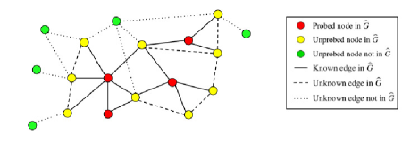
Figure 1: Overview of probing. Red nodes are already fully explored. The problem is to select yellow nodes (unprobed but in $\hat{G}$) that are adjacent to many green nodes (unprobed and not in $\hat{G}$).

Once $d^{out}_{u}$ has been calculated, MaxOutProbe selects the $b$ nodes with the highest such values (where $b$ is the probing budget).

We next describe how MaxOutProbe estimates each node $u$’s true degree $d_{u}$ as well as the graph’s average clustering coefficient $C$, which is used to estimate $d^{unknown}$ for each node. Section 3.2 describes how MaxOutProbe puts these various pieces together to obtain estimates for $d^{out}_{u}$.

3.1 MaxOutProbe’s Estimation Step

MaxOutProbe estimates (a) each candidate node $u$’s true degree $d_{u}$ and (b) the graph’s clustering coefficient $C$. Note that although there is a large body of work on estimating graph statistics, those works typically assume knowledge about how the graph was observed or generated (see Section 5). In contrast, MaxOutProbe makes no such assumptions. Instead to estimate the necessary statistics of $G$, MaxOutProbe performs a series of initial probes.

Estimating Node Degrees. We empirically observe that for incomplete networks, there exists some scale factor $f$ such that multiplying $u$’s sample degree by $\frac{1}{f}$ gives a good approximation of $d_{u}$. Thus, if MaxOutProbe estimates $f$, it can estimate the true degree $d_{u}$ of every node in the incomplete network by using that node’s observed degree. To perform this estimate, given a total probing budget of $b$, MaxOutProbe begins by identifying the $b$ candidate nodes from $\hat{G}$ with the highest degrees in $\hat{G}$. A small number of these nodes are randomly selected for probing, and their true degrees in $G$ are learned. By taking the average of the ratios of each selected node’s true degree to its degree in $\hat{G}$, MaxOutProbe estimates $f$.

Estimating Average Clustering Coefficient. Recall that the clustering coefficient of a node is the fraction of its neighbors that are connected, divided by the maximum possible such value. For a candidate node $u$, MaxOutProbe needs to know how many nodes that are presently two steps away from $u$ in $\hat{G}$ are likely to be connected to $u$ in $G$. Thus, rather than estimating the global average clustering coefficient or the average clustering coefficient for a candidate node, MaxOutProbe must estimate the average clustering coefficient for nodes that are adjacent to the candidate nodes. It is the clustering coefficient of these neighboring nodes that governs the number $d^{unknown}_{u}$. To make this estimation, MaxOutProbe uses the nodes selected for probing during the estimation of $f$, as described above. For each of these selected nodes $u$, MaxOutProbe considers each node $v$ that was two steps away in $\hat{G}$. MaxOutProbe then observes whether, after probing $u$, an edge connected $u$ to $v$. By averaging these results over all selected nodes $u$, MaxOutProbe estimates the average clustering coefficient.

Remarks. In cases when we know that the incomplete network was observed via random node sampling or random edge sampling, and know what fraction of the complete graph has been observed, it is possible to generate unbiased estimates for the degree of a candidate node and the clustering coefficient of the graph. The Appendix contains the proofs for these claims.

3.2 MaxOutProbe’s Selection Step

MaxOutProbe uses the estimates described above to select the $b$ candidate nodes that have the most unobserved neighbors. As before, $u$ is a (candidate) node in $\hat{G}$ that was not fully explored during the observation process. Let $f_{N}$ and $f_{E}$, respectively, denote the fraction of nodes and edges in $G$ that are present in $\hat{G}$. To estimate $d^{unknown}_{u}$, MaxOutProbe uses the knowledge that real-world social and information networks tend to exhibit high clustering (i.e., have lots of triangles). More precisely, let $w$ be an unexplored node that is two hops away from a candidate node $u$, such that $w$ and $u$ are not connected in $\hat{G}$ (but they may be connected in $G$). $w$ forms an open wedge with $u$, because $w$ and $u$ share at least one neighbor. Let $W_{u}$ be the number of such nodes $w$; these are the nodes in $\hat{G}$ to which $u$ is most likely connected. In the Estimation Step, MaxOutProbe estimated the average clustering coefficient $C$ of the network, which defines the fraction of wedges that are triangles (that is, the ratio of 3 times the number of triangles in the network to the number of length-2 paths in the network). Given this value, MaxOutProbe estimates that $u$ is connected to $C\times W_{u}$ nodes in $\hat{G}$, in addition to its known neighbors in $\hat{G}$.

Putting this all together, MaxOutProbe obtains the estimate for the number of neighbors that $u$ has outside of $\hat{G}$:

$$d^{out}_{u}=d_{u}-d^{known}_{u}-d^{unknown}_{u}=d_{u}-d^{known}_{u}-(C\times W_{u})$$ (2)

$d^{known}_{u}$ and $W_{u}$ can be calculated exactly from $\hat{G}$. The challenge thus lies in estimating $d_{u}$ and $C$, which was described in the Estimation Step above. MaxOutProbe computes $d^{out}_{u}$ for all candidate nodes in $\hat{G}$ and selects the $b$ candidate nodes with the highest $d^{out}$ values.

4 Experiments

Our experiments demonstrate that MaxOutProbe outperforms a variety of other probing methods with respect to the task of maximizing the number of nodes brought into the observed network, across incomplete networks observed by different popular sampling approaches.

Datasets. Table 1 describes the six real-world networks used in our experiments. Four are communications networks, and the other two are co-occurrence networks. The first co-occurrence network is an Amazon co-purchasing network with the nodes denoting books; and the second is a Youtube co-watching network with the nodes representing videos.

Type	Network $G$	# of Nodes	# of Edges	$G$’s Clust. Coeff.	# of Conn. Comp.
Communications	Enron Emails	84K	326K	0.08	950
Communications	Yahoo! IM	100K	595K	0.08	360
Communications	Twitter Replies	261K	309K	0.002	11,315
Communications	Twitter Retweets	40K	46K	0.03	3,896
Co-occurrences	Amazon Books	270K	741K	0.21	3840
Co-occurrences	Youtube Videos	167K	1M	0.007	1

Table 1: Statistics for the networks considered in our experiments. Clust. Coeff. is short for clustering coefficient. Conn. Comp. is short for connected components.

Sampling Methods. We observe incomplete networks using sampling methods, each corresponding to real application scenarios. For each sampling method, we select 10% of the edges from the original network. We consider the following sampling methods:

• RandNode: Nodes are sampled at random. The sample contains those nodes and all of their neighbors. This scenario corresponds to randomly selecting online accounts and observing all of their activities (such as all friendships or communications). This sampling method assumes that a list of observed nodes is available beforehand. Then, one node at a time is sampled until the sample reaches 10% of the total number of edges in the original network.

• RandEdge: Random edges are selected uniformly at random. Since edges are sampled, there is no assumption that a list of observed nodes is available beforehand. This is the scenario where one randomly observes communications (such as instant messages or emails).

• Random Walk (RW) and Random Walk w/ Jump (RWJ): These sampling methods begin at a random node and repeatedly transition to a random neighbor. In RWJ, at each step there is a chance (we use 15%) of jumping to a random node. A single edge at a time is observed. Thus, no assumption is made that a list of observed nodes is available beforehand. These are common sampling methods for large networks [12].

Other Popular Probing Methods. Table 2 describes a variety of probing methods, each with a simple scoring function for selecting nodes. These methods each rank all of the nodes in the incomplete graph $\hat{G}$ (except those that have already been fully explored). Some of the methods use exploit strategies, which heuristically select nodes, while others utilize explore strategies, which randomly select nodes. High degree probing relies on the intuition that high-degree nodes in $\hat{G}$ are connected to many nodes outside of $\hat{G}$. The structural hole methods target nodes that “fill” structural holes, thus connecting different parts of the graph [6]. On a similar intuition, the CrossComm algorithm selects nodes on the border of two communities. Random probing selects nodes at random from within $\hat{G}$ for probing.

Category	Sub-category	Name	Description
Exploit	Degree	HighDeg, LowDeg	Select the highest or lowest degree nodes.
	Structural Hole	HighDisp, LowDisp	Select the highest or lowest dispersion nodes [4].
		CrossComm	Pick nodes with the highest fraction of neighbors outside of
			their community (as identified with the Louvain method [5]).
	Clustering	HighCC, LowCC	Select the highest or lowest clustering coefficient nodes.
Explore		Random	Randomly select nodes from the sample.

Table 2: Other popular probing methods. We categorize methods as explore or exploit, and further subdivide as degree based, structural hole based, or random. Dispersion is an edge-based measure of how well a node’s neighbors are connected to each other [4]. For each node, we average the dispersion of each of its adjacent edges.

Experimental Setup. For each network listed in Table 1, we generate 20 incomplete networks using each of the four sampling methods described above. Each incomplete network contains 10% of the edges from the original network. For each probing method, we conduct probes at budgets $b\in\left\{1\%,2\%,3\%,4\%,5\%\right\}$ of the number of nodes in $G$. After conducting probes on an incomplete network $\hat{G}$, we obtain an augmented sample graph $\hat{G^{\prime}}$. To evaluate the quality of $\hat{G^{\prime}}$, we simply count how many nodes it has.

Results. First, we evaluate MaxOutProbe and the other popular probing methods on the incomplete networks described above. We observe that averaged over the 20 incomplete networks, for every sampling method and every network, MaxOutProbe matches or outperforms the best popular probing method. For example, see Figure 2(a), which shows the performances of various probing methods on incomplete networks observed by random node sampling on the Yahoo! IM network. In some cases, MaxOutProbe performs roughly the same as High Degree probing (see, e.g., Figure 2(b), for results on incomplete samples observed by random walk sampling on the Twitter Replies network). This occurs when the incomplete network has a very low estimated clustering coefficient. On these incomplete networks, MaxOutProbe estimated average clustering coefficients ranges from 0.0 to 0.03. With such a low clustering coefficient, MaxOutProbe reduces to effectively picking the nodes with the highest observed degrees.

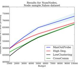
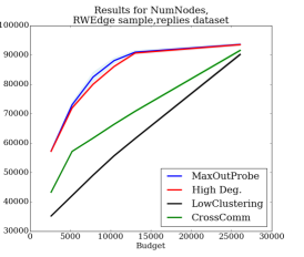
(a)	(b)

Figure 2: Results of MaxOutProbe vs. popular probing methods on incomplete networks. In (a), twenty networks were observed by random node sampling on the Yahoo! IM network. Shading indicates one standard deviation. Observe that MaxOutProbe is the best across all considered node budgets. In (b), twenty networks were observed by random walk sampling on the Twitter Replies network. Shading indicates one standard deviation. Observe that MaxOutProbe and High Degree probing perform similarly because the Twitter Replies network has a very low clustering coefficient (of 0.002). Results on the other datasets and sampling methods are similar to these and have been removed for brevity.

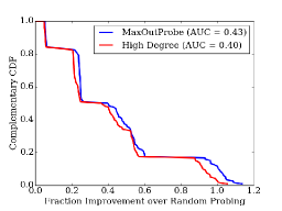
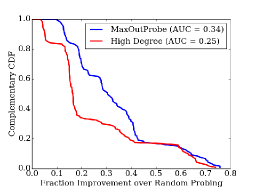
(a) Observed by Random Edge Sampling	(b) Observed by Random Node Sampling
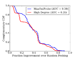
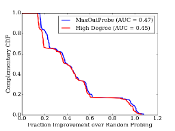
(c) Observed by Random Walks	(d) Observed by Random Walks with Jumps

Figure 3: Complementary CDFs showing results of MaxOutProbe and High Degree probing as compared to Random probing across all datasets, on incomplete networks observed by various sampling methods. In all cases, MaxOutProbe has a higher area under the curve (AUC), indicating a greater improvement over Random probing than High Degree probing.

Rather than present plots for each network and sampling method, we aggregate results across datasets, comparing MaxOutProbe to High Degree probing (which is typically the best popular probing method). For each incomplete network and each considered budget, we conduct probes using MaxOutProbe and High Degree probing, and count the number of nodes in each resulting $\hat{G^{\prime}}$. Because we cannot meaningfully compare these numbers across datasets or sampling methods, we also conduct the same number of probes using Random probing, and then calculate the percent by which MaxOutProbe and High Degree probing improved over Random probing (i.e., how much larger is the $\hat{G^{\prime}}$ produced by MaxOutProbe or High Degree probing versus that produced by Random probing?). By comparing to Random probing, we are able to make sensible comparisons across datasets. Figure 3 shows complementary CDFs of these aggregate results at the 0.05 probing budget on incomplete networks observed, respectively, by Random Edge sampling, Random Node sampling, Random Walk sampling, and Random Walk with Jump sampling. Similar results were observed at other probing budgets. The x-axis represents the percent improvement over Random probing, with values greater than 0 indicating that the approach performed better than Random probing. The y-axis represents the fraction of such results that produced at least a certain fraction improvement over random. We see that in all cases, MaxOutProbe has a higher area under the curve than High Degree probing, indicating greater improvement. The area under the curve for MaxOutProbe ranges from 4% to 36% higher than that of High Degree probing.

5 Related Work

Our work is most related to graph sampling and crawling. There is a rich literature on sampling graphs. For instance, previous literature has examined the study of community detection from graph samples$-$e.g., by using minimum spanning trees (MSTs) [20], or by expanding a graph sample [14]. Avrachenkov et al. [3] use queries to locate high-degree nodes. O’Brien and Sullivan [16] use local information to estimate the core number of a node. Hanneke and Xing [9] and Kim and Leskovec [11] infer characteristics of a larger graph given a sample. Maiya and Berger-Wolf [15] study the problem of online sampling for centrality measures. Cho et al. [7] study the problem of determining which URLs to examine in a Web crawl. In contrast, we study the problem of selecting which nodes from an existing incomplete network one should probe, rather than constructing a sample from scratch. Also, unlike many sampling methods, we are not down-sampling a network to which we have complete access, but using a limited number of probes.

MaxOutProbe selects probes in a batch, not incremental, manner. This difference is critical when obtaining data is time-consuming. The closest method to MaxOutProbe is the MEUD (Maximum Expected Uncovered Degree) algorithm by Avrachenkov et al. [2]: a sampling method intended to bring as many nodes as possible into the sample. MEUD begins with one node; then in each step, it grows the sample by adding the node with the highest expected degree in the underlying, unobserved network. MEUD requires knowing the degree distribution of the underlying network, but for certain classes of graphs, reduces to selecting the nodes with the highest observed degrees. This is a valid approximation only for limited classes of random graphs, while our proposed method does not have such constraints. Note that if we modified the MEUD algorithm to fit our problem setting, it would be reduce to High Degree probing.

Researchers interested in specific network features have studied related problems. Macskassy and Provost [13] address the problem of identifying malicious entities in incomplete networks by gathering more information about suspicious entities. Cohen et al. [8] propose an approach for immunizing a population in an unobserved network by targeting neighbors of randomly selected nodes. Shakkottai [18] considers the problem of nodes in a sensor network attempting to find the source of information. Ragoler et al. [17] study the problem of determining the frequency at which sensor nodes should query their environments. Lastly, graph theoreticians have studied the testability of certain graph properties (such as monotone graph properties [1]).

6 Conclusions

We discussed the problem of determining which nodes in an incomplete network should be probed in order to maximize the number of new nodes observed. We presented the MaxOutProbe algorithm, which estimates the degree of each observed but unexplored node, as well as the graph’s average clustering coefficient, to rank nodes for probing. We demonstrated that MaxOutProbe outperforms several popular probing methods on incomplete networks observed by four popular sampling methods over six network datasets. Where the graph has a very low clustering coefficient, MaxOutProbe’s performance is similar to selecting nodes with the highest observed degree.

Appendix

Suppose we know the fraction of nodes $f_{N}$ and the fraction of edges $f_{E}$ of $G$ that are in $\hat{G}$; and we know that the incomplete network was observed via random node or random edge sampling. Under such conditions, MaxOutProbe produces unbiased estimates for the node degrees and the global clustering coefficient of the network without having to use some of the probing budget to produce these estimates. This section contains the proofs for these claims.

Estimations for Known Random Node Samples

In random node sampling, $f_{N}$ fraction of the nodes in $G$ are selected at random and all their neighbors are collected. Suppose node $u$ is in the observed network, but was not one of the nodes selected at random (that is, $u$ was observed because one of its neighbors was selected). If node $u$ has observed degree $d^{known}_{u}$ in $\hat{G}$, MaxOutProbe estimates its true degree as $\frac{1}{f_{N}}d^{known}_{u}$. For example, if $u$ is adjacent to 5 nodes in $\hat{G}$, and 10% of the nodes from $G$ were selected during sampling, then MaxOutProbe estimates $u$’s true degree $d_{u}$ as 50. This estimation works well for high degree nodes, but is less accurate for low degree nodes. However, as we saw in Section 4, probing low degree nodes in $\hat{G}$ is unlikely to lead to a large number of new nodes being observed.

Claim #1: MaxOutProbe’s estimator for $d_{u}$ is unbiased under random node sampling.

Proof: We know that $\hat{G}$ consists of $f_{N}$ fraction of the nodes in $G$ selected uniformly at random, plus the neighbors of these selected nodes. Let $\hat{d_{u}}$ represent the estimator for $d_{u}$. MaxOutProbe sets $\hat{d_{u}}$ to be $\frac{1}{f_{N}}d^{known}_{u}$, where $d^{known}_{u}$ is the observed degree of node $u$ in $\hat{G}$. We must show that for each $u$, $\mathbb{E}[\hat{d_{u}}]=d_{u}$.

Consider a node $u$ that has not been explored during the sampling process, but is present in the sample $\hat{G}$ (that is, $u$ is adjacent to a node that was explored during sampling). Node $u$ has $d_{u}$ neighbors in $G$, and because $f_{N}$ of the nodes from $G$ were sampled uniformly at random to produce $\hat{G}$, $\mathbb{E}[d^{known}_{u}]=f_{N}d_{u}$. Thus, $\frac{1}{f_{N}}\mathbb{E}[d^{known}_{u}]=d_{u}$, or equivalently $\mathbb{E}[\frac{1}{f_{N}}d^{known}_{u}]=d_{u}$. Since $\hat{d_{u}}=\frac{1}{f_{N}}d^{known}_{u}$, we have $\mathbb{E}[\hat{d_{u}}]=d_{u}$, indicating that $\hat{d_{u}}$ is an unbiased estimator for $d_{u}$. $\blacksquare$

To estimate the global clustering coefficient $C$ of $G$, MaxOutProbe estimates the number of wedges (i.e., length-2 paths) and triangles in $G$. Let $T_{\hat{G}}$ and $W_{\hat{G}}$ represent, respectively, the number of triangles and wedges in $\hat{G}$, and let $C_{\hat{G}}=3\frac{T_{\hat{G}}}{W_{\hat{G}}}$ be the observed global clustering coefficient of $\hat{G}$.

Suppose a triangle consisting of nodes $x$, $y$, and $z$ exists in $G$. What is the probability that it is in $\hat{G}$? If all edges $(x,y),(y,z)$, and $(x,z)$ are in $\hat{G}$, then at least one node from each of these three edges must be fully explored during sampling. Thus, the triangle will be in $\hat{G}$ if and only if at least two of the three nodes are selected. We can write the probability $p_{T}$ that this occurs as:

$$p_{T}=3f^{2}_{N}(1-f_{N})+f^{3}_{N}$$ (3)

In other words, $p_{T}$ is the probability that exactly two of the three nodes are selected, plus the probability that all three are selected. Thus, by multiplying the observed number of triangles in $\hat{G}$ by $\frac{1}{p_{T}}$, MaxOutProbe estimates the number of triangles $T$ in $G$ as:

$$T=\frac{T_{\hat{G}}}{p_{T}}.$$ (4)

We also need to calculate the probability that a length-2 path $\{(x,y),(y,z)\}$ in $G$ also appears in $\hat{G}$ ($x$ may or may not be connected to $z$). If this path is in $\hat{G}$, either at least two nodes from $\{x,y,z\}$ were sampled, or $y$ must be sampled. The probability $p_{W}$ of this occurring is as follows:

$$p_{W}=f^{3}_{N}+3(f^{2}_{N}(1-f_{N}))+f_{N}(1-f_{N})^{2}$$ (5)

This is the probability that all three nodes are sampled plus the probability that exactly two nodes are sampled plus the probability that just $y$ is sampled. MaxOutProbe then multiplies the observed number of length-2 paths from $\hat{G}$ by $\frac{1}{p_{W}}$ to estimate the number of wedges $W$ in $G$ as:

$$W=\frac{W_{\hat{G}}}{p_{W}}.$$ (6)

$G$’s global clustering coefficient is estimated as $\hat{C}=3\frac{T}{W}=3(\frac{T_{\hat{G}}}{p_{T}})/(\frac{W_{\hat{G}}}{p_{W}})=3\frac{p_{W}}{p_{T}}\frac{T_{\hat{G}}}{W_{\hat{G}}}=\frac{p_{W}}{p_{T}}C_{\hat{G}}$.

Claim #2: MaxOutProbe’s estimator for $C$ is an unbiased estimate of the graph’s true global clustering coefficient under random node sampling.

Proof: $\hat{G}$ consists of $f_{N}$ fraction of the nodes in $G$ selected uniformly at random, plus the neighbors of these selected nodes. Let $\hat{C}$ represent the estimator for $G$’s true global clustering coefficient $C$. MaxOutProbe sets $\hat{C}$ to be $\frac{p_{W}}{p_{T}}C_{\hat{G}}$, as described above. We must show that $\mathbb{E}[\hat{C}]=C$.

Suppose that the wedge $\{(x,y),(y,z)\}$ appears in $\hat{G}$. Also, suppose that the nodes $x$, $y$, and $z$ form a triangle in $G$ (i.e., edge $(x,z)$ is present in $G$). What is the probability that edge $(x,z)$ is present in $\hat{G}$ (i.e., the nodes $x$, $y$, and $z$ form a triangle in $\hat{G}$)? Because we assume that the wedge $\{(x,y),(y,z\}$ is present in $\hat{G}$, some of these three nodes must have been selected during the sampling process. Thus, we need to consider three possibilities:

1. All three of $x,y,z$ were sampled. The probability of this occurring is $f_{N}^{3}$.

2. Exactly two of $x$, $y$, and $z$ were sampled. The probability of this occurring is $3f_{N}^{2}(1-f_{N})$.

3. Only $y$ was sampled. The probability of this occurring is $f_{N}(1-f_{N})^{2}$.

In possibilities (1) and (2), edge $(x,z)$ will certainly be present in $\hat{G}$. In possibility (3), edge $(x,z)$ will not be present in $\hat{G}$. Thus, given that the wedge $\{(x,y),(y,z)\}$ is present in $\hat{G}$, the probability $P_{closed}$ that edge $(x,z)$ is also present in $\hat{G}$ is as follows:

$$P_{closed}=\frac{f_{N}^{3}+3f_{N}^{2}(1-f_{N})}{f_{N}^{3}+3f_{N}^{2}(1-f_{N})+f_{N}(1-f_{N})^{2}}=\frac{p_{T}}{p_{W}}$$ (7)

Thus, given that a set of nodes forms a wedge in $\hat{G}$ and a triangle in $G$, $P_{closed}$ is the probability that it also forms a triangle in $\hat{G}$. In other words, $\mathbb{E}[C_{\hat{G}}]=P_{closed}{C}=\frac{p_{T}}{p_{W}}{C}$. Since the definition of $\hat{C}$ is simply $\frac{p_{W}}{p_{T}}C_{\hat{G}}$, we have that $\mathbb{E}[\hat{C}]=C$, so $\hat{C}$ is an unbiased estimator of $C$. $\blacksquare$

Estimations for Known Random Edge Samples

In random edge sampling, $f_{E}$ fraction of edges are sampled uniformly at random. To estimate a node’s true degree $d_{u}$, MaxOutProbe multiplies its observed degree $d^{known}_{u}$ by $\frac{1}{f_{E}}$. As with random node sampling, this estimation is inaccurate for low degree nodes, but such nodes are unlikely to be selected, and this inaccuracy does not affect MaxOutProbe’s selection of nodes to probe.

Claim #3: MaxOutProbe’s estimator for $d_{u}$ is unbiased under random edge sampling.

Proof: We know that $\hat{G}$ consists of a fraction $f_{E}$ of the edges in $G$ selected uniformly at random. Let $\hat{d_{u}}$ represent the estimator for $d_{u}$. MaxOutProbe sets $\hat{d_{u}}$ to be $\frac{1}{f_{E}}d^{known}_{u}$, where $d^{known}_{u}$ is the observed degree of node $u$ in $\hat{G}$. We must show that for each $u$, $\mathbb{E}[\hat{d_{u}}]=d_{u}$.

Consider a node $u$ in $\hat{G}$, with true degree $d_{u}$. Because $f_{E}$ of the edges from $G$ were sampled uniformly at random, $\mathbb{E}[d^{known}_{u}]=f_{E}d_{u}$, or equivalently $\mathbb{E}[\frac{1}{f_{E}}d^{known}_{u}]=d_{u}$. Therefore, $\mathbb{E}[\hat{d_{u}}]=d_{u}$, indicating that $\hat{d_{u}}$ is an unbiased estimator for $d_{u}$. $\blacksquare$

Consider a length-2 path $\{(x,y),(y,z)\}$ in $G$ that is present in $\hat{G}$. If $x$ is connected to $z$ in $G$ (i.e., there exists a triangle between $x$, $y$, and $z$ in $G$), then with probability $f_{E}$, edge $(x,z)$ is also present in $\hat{G}$. Thus, MaxOutProbe estimates $C$ (the global clustering coefficient of $G$) to be $\frac{1}{f_{E}}C_{\hat{G}}$, where $C_{\hat{G}}$ is the global clustering coefficient of the incomplete network $\hat{G}$.

Claim #4: MaxOutProbe’s estimator for $C$ is unbiased under random edge sampling.

Proof: We know that $\hat{G}$ consists of a fraction $f_{E}$ of the edges in $G$ selected uniformly at random. Let $\hat{C}$ represent the estimator for $C$. MaxOutProbe sets $\hat{C}$ to be $\frac{1}{f_{E}}C_{\hat{G}}$, where $C_{\hat{G}}$ is the global clustering coefficient of the incomplete network $\hat{G}$. We must show that $\mathbb{E}[\hat{C}]=C$.

$C$ is the fraction of wedges (i.e., length-2 paths $\{(x,y),(y,z)\}$) that are closed (i.e., $x$ is connected to $z$). Suppose that the edge $(x,z)$ exists in $G$. Then, independently of the wedge $\{(x,y),(y,z)\}$ being present in $\hat{G}$, there is $f_{E}$ probability that $(x,z)$ is present in $\hat{G}$. Thus, of the wedges in $G$ that are present in $\hat{G}$, we expect that $f_{E}C$ fraction of these wedges are closed in $\hat{G}$. If $C_{\hat{G}}$ is the global clustering coefficient of $\hat{G}$, then $\mathbb{E}[C_{\hat{G}}]=f_{E}C$, or equivalently $\mathbb{E}[\frac{1}{f_{E}}C_{\hat{G}}]=C$. Therefore, $\mathbb{E}[\hat{C}]=C$, indicating that $\hat{C}$ is an unbiased estimator for $C$. $\blacksquare$

Remarks

The aforementioned proofs (for both random node and random edge sampling) show that the estimates are correct in expectation, but do not provide concentration bounds. By applying Hoeffding’s inequality [10], we can bound the errors in expectations. While these bounds may be weak for each node, they provide a theoretical basis for showing that we can identify all high-degree nodes up to some approximation (see Theorem 6.2 in [19]).

References

- [1] N. Alon and A. Shapira. Every montone graph property is testable. SIAM J. Comput., 38(2):505–522, 2008.
- [2] K. Avrachenkov, P. Basu, G. Neglia, B. Ribeiro, and D. Towsley. Pay few, influence most: Online myopic network covering. In IEEE NetSciCom Workshop, 2014.
- [3] K. Avrachenkov, N. Litvak, L. O. Prokhorenkova, and E. Sayargulova. Quick detection of high-degree entities in large directed networks. In ICDM, pages 20–29, 2014.
- [4] L. Backstrom and J. Kleinberg. Romantic partnerships and the dispersion of social ties: a network analysis of relationship status on facebook. In CSCW, pages 831–841, 2014.
- [5] V.D. Blondel, J.-L. Guillaume, R. Lambiotte, and E. Lefebvre. Fast unfolding of communities in large networks. J. Stat. Mech., page 10008, 2008.
- [6] R.S. Burt. The social capital of structural holes. In M. F. Guillen, R. Collins, P. England, and M. Meyer, editors, New Directions in Economic Sociology. Russell Sage Foundation, 2002.
- [7] J. Cho, H. Garcia-Molina, and L. Page. Efficient crawling through URL ordering. In WWW, pages 161–172, 1998.
- [8] R. Cohen, S. Havlin, and D. Ben-Avraham. Efficient immunization strategies for computer networks and populations. Phys. Rev. Lett., 91(24):247901, 2003.
- [9] S. Hanneke and E.P. Xing. Network completing and survey sampling. In AISTATS, pages 209–215, 2009.
- [10] W. Hoeffding. Probability inequalities for sums of bounded random variables. J. American Statistical Association, 58(30):13–30, 1963.
- [11] M. Kim and J. Leskovec. The network completion problem: Inferring missing nodes and edges in networks. In SDM, pages 47–58, 2011.
- [12] J. Leskovec and C. Faloutsos. Sampling from large graphs. In KDD, pages 631–636, 2006.
- [13] S. Macskassy and F. Provost. Suspicion scoring based on guilt-by-association, collective inference, and focused data access. In Int’l Conf. on Intell. Analysis, 2005.
- [14] A.S. Maiya and T. Berger-Wolf. Sampling community structure. In WWW, pages 701–710, 2010.
- [15] A.S. Maiya and T. Berger-Wolf. Online sampling of high centrality individuals in social networks. In PAKDD, pages 91–98, 2010.
- [16] M.P. O’Brien and B.D. Sullivan. Locally estimating core numbers. In ICDM, pages 460–469, 2014.
- [17] I. Ragoler, Y. Matias, and N. Aviram. Adaptive probing and communication in sensor networks. In ADHOC-NOW, volume 3158, pages 280–293, 2004.
- [18] S. Shakkottai. Asymptotics of query strategies over a sensor network. In INFOCOM, pages 548–557, 2004.
- [19] D. Thompson, J. Bennett, C. Seshadhri, and A. Pinar. A provably-robust sampling method for generating colormaps of large data. In LDAV, pages 77–84, 2013.
- [20] J. Wu, X. Li, L. Jiao, X. Wang, and B. Sun. Minimum spanning trees for community detection. Physica A, 392(9):2265–2277, 2013.