Formation probabilities and Shannon information and their time evolution after quantum quench in transverse-field XY-chain

Abstract

We first provide a formula to calculate the probability of occurrence of different configurations (formation probabilities) in a generic free fermion system. We then study the scaling of these probabilities with respect to the size in the case of critical transverse-field XY-chain in the $\sigma^{z}$ bases. In the case of the transverse field Ising model, we show that all the ”crystal” configurations follow the formulas expected from conformal field theory (CFT). In the case of critical $XX$ chain, we show that the only configurations that follow the formulas of the CFT are the ones which respect the filling factor of the system. By repeating all the calculations in the presence of open and periodic boundary conditions we find further support to our classification of different configurations. Using the developed technique, we also study Shannon information of a subregion in our system. In this respect we distinguish particular configurations that are more important in the study of the scaling limit of the Shannon information of the subsystem. Finally, we study the evolution of formation probabilities, Shannon information and Shannon mutual information after a quantum quench in free fermion system. In particular, for the intial state considered in this paper, we demonstrate that the Shannon information after quantum quench first increases with the time and then saturates at time $t^{*}=\frac{l}{2}$, where $l$ is the size of the subsystem.

I Introduction

Studying correlation functions in many-body systems has been considered one of the main topics in statistical mechanics and condensed matter physics for many years. Although, for a long-time the main quantities of interest were the correlation functions of local observables the recent interest in calculating non-local quantities, especially the entanglement entropy, has made significant changes. One of the main reasons for this interest (at least in $1+1$ dimensional critical systems) is that by calculating some of the non-local observables one can derive the central charge of the system without referring to the velocity of sound, for the case of entanglement entropy see CC2009 . Another non-local quantity which has been studied for many years with Bethe ansatz techniques and some other methods is emptiness formation probability Essler ; U1 ; Shiroishi ; Abanov-Korepin; Franchini ; Stephan2013 . In the case of spin chains, it is the probability of finding a sequence of up spins in the system (note that almost all of the studies in this regard concentrate on the $\sigma^{z}$ bases). These studies show that this probability, with respect to the sequence size, decreases like a Gaussian in the case of systems with $U(1)$ symmetry U1 and exponentially in other cases Shiroishi ; Franchini . In the critical cases, the Gaussian and exponential are accompanied with a power-law decay with a universal exponent. In a recent development Stephan2013 it was shown that for those critical systems without $U(1)$ symmetry this universal exponent is dependent on the central charge of the system. The argument is based on connecting the configuration of all spins up to some sort of boundary conformal field theory. One should notice that the argument works just for those bases that can be connected to boundary conformal field theory.

In an apparently connected studies recently many authors investigated the Shannon information of quantum systems in different systems Stephan2009 ; Stephan2010 ; Oshikawa2010 ; Stephan2011 ; Alet2013 ; Alet2014a ; Alet2014b ; Alet2014c ; Trebst2014 ; Trebst2015 ; Jose . The Shannon information is defined as follows: Consider the normalized ground state eigenfunction of a quantum spin chain Hamiltonian $|\psi_{G}\rangle=\sum_{I}a_{I}|I\rangle$, expressed in a particular local bases $|I\rangle=|i_{1},i_{2},\cdots\rangle$, where $i_{1},i_{2},\cdots$ are the eigenvalues of some local operators defined on the lattice sites. The Shannon entropy is defined as

$$Sh=-\sum_{I}p_{I}\ln p_{I},$$ (1)

where $p_{I}=|a_{I}|^{2}$ is the probability of finding the system in the particular configuration given by $|I\rangle$. As it is quite clear this quantity is bases dependent and to calculate it one needs in principle to know the probability of occurrence of all the configurations. The number of all configurations increases exponentially with the size of the system and that makes analytical and numerical calculations of this quantity quite difficult. Note that the emptiness formation probability is just one of the whole possible configurations. The Shannon information of the system changes like a volume law with respect to the size of the system so in principle one does not expect to extract any universal information by studying the leading term. The universal quantities should come from the subleading terms. To study subleading terms, it is useful to define yet another quantity called Shannon mutual information. By considering local bases it is always possible to decompose the configurations as a combination of the configurations inside and outside of a subregion $A$ as $|I\rangle=|I_{A}I_{\bar{A}}\rangle$. Then one can define the marginal probabilities as $p_{I_{A}}=\sum_{I_{\bar{A}}}p_{I_{A}I_{\bar{A}}}$ and $p_{I_{\bar{A}}}=\sum_{I_{A}}p_{I_{A}I_{\bar{A}}}$ for the subregion $A$ and its complement $\bar{A}$. Then the Shannon mutual information is

$$I(A,\bar{A})=Sh(A)+Sh(\bar{A})-Sh(A\cup\bar{A}),$$ (2)

where $Sh(A)$ and $Sh(\bar{A})$ are the Shannon informations of the subregions $A$ and $\bar{A}$. From now on instead of using $p_{I_{A}I_{\bar{A}}}$ we will use just $p_{I}$. Since in the above quantity the volume part of the Shannon entropy disappears Shannon mutual information provides a useful technique to study the subleading terms. Note that one can similarly define the above quantity also for two regions $A$ and $B$, i.e. $I(A,B)$ that are not necessarily complement of each other. The Shannon mutual information has been studied in many classical Wolf2008 ; wilms ; Grassberger ; Rittenberg2014 and quantum systems Um ; AR2013 ; Stephan2014 ; AR2014 ; AR2015 . Numerical studies on variety of different periodic quantum critical spin chains show that for particular bases (so called conformal bases) we have AR2013 ; AR2014 ; AR2015

$$I(A,\bar{A})=\beta\ln[\frac{L}{\pi}\sin(\frac{\pi l}{L})],$$ (3)

where $L$ and $l$ are the total size and subsystem size respectively and $\beta$ is very close to $\frac{c}{4}$, with $c$ the central charge of the system. Note that if one takes an arbitrary base (non-conformal bases) the coefficient $\beta$ is nothing to do with the central charge. It is worth mentioning that based on AR2014 the conformal bases are those bases that can be connected to some sort of boundary conformal field theory in the sense of Stephan2013 . For example in the transverse field Ising model the $\sigma^{x}$ and $\sigma^{z}$ bases are the conformal bases. Note that if one considers the Shannon information of the subsystem we will have $Sh(A)=\alpha l+\beta\ln[\frac{L}{\pi}\sin(\frac{\pi l}{L})]$. Since to extract the Shannon information one needs to use all the probabilities the only way to consider all of them in the numerical calculations is exact diagonalization. This makes the numerical calculation for large sizes very difficult. The results of the articles AR2013 ; AR2014 ; AR2015 are all for periodic systems with $L=30$ whenever there are spin one-half system and smaller sizes for systems with bigger spins. In a recent work Stephan2014 the author was able to consider an infinite system and study the Shannon information of the subsystem up to the size $l=40$. It was concluded that for the $XX$ chain $\beta$ is $\frac{c}{4}$ with $c=1$ but for the Ising model although it is very close to $\frac{c}{4}$ with $c=\frac{1}{2}$ the results are suggesting that probably $\beta$ is not exactly connected to the central charge. Notice that all of the above calculations are done by considering periodic boundary conditions for the connected regions $A$ and $\bar{A}$. It is not clear how the equation (3) might change if one considers open boundary conditions. Finally it is worth mentioning that some of the the above results have recently been extended to disconnected regions in Rajabpour2015d .

Motivated by the studies of emptiness formation probability and Shannon information of the subsystem we study here some related quantities. First of all, as it is natural one might be interested in studying the scaling limit of some other configurations with respect to the size of the subsystem. For example, consider an antiferromagnetic configuration in the Ising model or any other configuration with pattern. It is very important to know that these configurations are also flowing to some sort of boundary conformal field theory or not. This study will clearly also help to understand the nature of the Shannon mutual information. In addition, this kind of studies also are very useful in the calculations of post-measurement entanglement entropy and localizable entanglement entropy Rajabpour2015b ; Rajabpour2015c . Having the above motivations in mind, we study formation probabilities , Shannon information and their evolution after a quantum quench in the quantum $XY$ chain in the $\sigma^{z}$ bases.

The outline of the paper is as follows: In the next section we will first define our system of interest, i.e. $XY$ chain and then we will provide a method to calculate the probability of any configuration in the free fermionic systems. In section three we will list all the known analytical results regarding emptiness formation probability for infinite systems and also finite systems with periodic and open boundary conditions. Explicit distinguishment is made between critical Ising model and $XX$ chain with $U(1)$ symmetry. In section IV, we will define many different configurations with specially defined pattern and calculate their corresponding probabilities numerically. Here again, we discuss Ising and $XX$ universalities separately for infinite systems and for the systems with boundary. We also discuss configurations that do not have any pattern. In section V, we study the Shannon information in the transverse field critical Ising model and also critical $XX$ chain. We will classify the configurations based on their magnetization and show that in principle just a small part of the configurations can have a finite contribution to Shannon information in the scaling limit. Section VI is devoted to the evolution of formation probabilities and Shannon information after a quantum quench. We prepare the system in a particular state and then we let it evolve with another Hamiltonian and study the time evolution of the formation probabilities and especially Shannon information. Finally, the last section is about our conclusions and possible future works.

II Formation probabilities from reduced density matrix

In this section, we first define the system of interest and after that using the reduced density matrix of this system we will find a very efficient method to calculate formation probabilities for systems that can be mapped to free fermions. The Hamiltonian of the XY-chain is as follows:

$$H=-\sum_{j=1}^{L}\Big{[}(\frac{1+a}{2})\sigma_{j}^{x}\sigma_{j+1}^{x}+(\frac{1-a}{2})\sigma_{j}^{y}\sigma_{j+1}^{y}+h\sigma_{j}^{z}\Big{]}.$$ (4)

After using Jordan-Wigner transformation, i.e. $c_{j}=\prod_{{}_{m<j}}\sigma_{m}^{z}\frac{\sigma_{j}^{x}-i\sigma_{j}^{y}}{2}$ and $\mathcal{N}=\prod_{{}_{m=1}}^{{}^{L}}\sigma_{m}^{z}=\pm 1$ with $c_{L+1}^{\dagger}=0$ and $c_{L+1}^{\dagger}=\mathcal{N}c_{1}^{\dagger}$ for open and periodic boundary conditions respectively the Hamiltonian will have the following form:

$$H=\sum_{j=1}^{L}\Big{[}(c_{j}^{\dagger}c_{j+1}+ac_{j}^{\dagger}c_{j+1}^{\dagger}+h.c.)-h(2c_{j}^{\dagger}c_{j}-1)\Big{]}+\mathcal{N}(c_{L}^{\dagger}c_{1}+ac_{L}^{\dagger}c_{1}^{\dagger}+h.c.).$$ (5)

The above Hamiltonian has a very rich phase space with different critical regions Mccoy1971 . In figure  1 we show different critical regions of the system. To calculate probability of formations for different patterns we first write the reduced density matrix of a block of spins $D$ by using block Green matrices. Following Peschela ; Barthel2008 we first define the operators

$$a_{i}=c_{i}^{\dagger}+c_{i},\hskip 28.45274ptb_{i}=c_{i}^{\dagger}-c_{i}.$$ (6)

The block Green matrix is defined as

$$G_{ij}={\rm tr}\,[\rho_{D}b_{i}a_{j}].$$ (7)

The elements of the Green matrix can be calculated following Lieb and we will mention their explicit form for open and periodic boundary conditions later.

Figure 1: (Color online) Different critical regions in quantum $XY$ chain. The critical $XX$ chain has central charge $c=1$ and critical $XY$ chain has $c=\frac{1}{2}$.

To calculate the reduced density matrix after partial measurement we need to first define fermionic coherent states. They can be defined as follows

$$|\boldsymbol{\xi}>=|\xi_{1},\xi_{2},...,\xi_{N}>=e^{-\sum_{i=1}^{N}\xi_{i}c_{i}^{\dagger}}|0>,$$ (8)

where $\xi_{i}$’s are Grassmann numbers following the properties: $\xi_{n}\xi_{m}+\xi_{m}\xi_{n}=0$ and $\xi_{n}^{2}=\xi_{m}^{2}=0$. Then it is easy to show that

$$c_{i}|\boldsymbol{\xi}>=-\xi_{i}|\boldsymbol{\xi}>.$$ (9)

Using the coherent states (8) the reduced density matrix has the following form Barthel2008

$$\rho_{D}(\boldsymbol{\xi},\boldsymbol{\xi^{\prime}}) = <\boldsymbol{\xi}|\rho_{D}|\boldsymbol{\xi^{\prime}}>$$ (10)

$$= \det\frac{1}{2}(1-G)e^{\frac{1}{2}(\boldsymbol{\xi}^{*}-\boldsymbol{\xi}^{\prime})^{T}F(\boldsymbol{\xi}^{*}+\boldsymbol{\xi}^{\prime})},$$

where $F=(G+1)(1-G)^{-1}$. One can use the above formula to extract the formation probability for arbitrary configuration in the $\sigma_{z}$ bases as follows: first of all to extract the probability of particular configuration we need to look to the diagonal elements of $\rho_{D}(\boldsymbol{\xi},\boldsymbol{\xi^{\prime}})$. When the spin in the $\sigma^{z}$ direction is up in the fermionic representation it can be understood as the lack of a fermion in that site which in the language of coherent states means that the corresponding $\xi$ is zero in the equation (10). After putting some of the $\xi$’s equal to zero one will have a new reduced density matrix in the coherent state basis with this constraint that some of the spins are fixed to be up. In other words in the equation (10) instead of $F$ we will have $\tilde{F}$ which is a sub-matrix of the matrix $F$. The elements of the new reduced density matrix will be $\tilde{\rho}_{D}(\boldsymbol{\eta},\boldsymbol{\eta^{\prime}})$, where we put the $\xi$’s corresponding to the sites filled with fermions equal to $\eta$. To extract the probability of formation one just needs to integrate over all the $\eta$’s that correspond to the down spins. In other words after using formulas of the Grassmann Gaussian integrals the formation probability will have the following formula

$$P(\mathcal{C}_{n})=\det[\frac{1}{2}(1-G)]M_{F}^{\mathcal{C}_{n}},$$ (11)

where $M_{F}^{\mathcal{C}_{n}}$ is the minor of the matrix $F$ corresponding to the configuration $\mathcal{C}_{n}$. Notice that we just need principal minors of the matrix $F$. Since the sum of all the principal minors of the matrix $F$ is equal to $\det(1+F)$ the normalization is ensured. We have $\binom{l}{k}$ number of rank-k minors for matrix $F$ with size $l$. Summing over the number of all principal minors, one can obtain $2^{l}$ which is the number of all possible configurations. Configurations with the same minor rank have the same number of up spins and by increasing $k$ we actually increase the number of down spins in the corresponding configuration. For example $k=0(l)$ is the case with all spins up (down) and sometimes it is called emptiness formation. The above formula gives a very efficient way to calculate the formation probabilities in numerical approach. Since, as we will show, all of these probabilities are exponentially small with respect to the size of the subsystem it is much easier to work with the logarithm of them and define logarithmic formation probabilities

$$\Pi(\mathcal{C}_{n})=-\ln P(\mathcal{C}_{n}).$$ (12)

All of the calculations done in this paper are based on the formula (11) and are performed using Mathematica. In the next sections, we will study the formation probabilities for different configurations with the crystal order (pattern formation probabilities) with respect to the size of the subsystem for some particular critical regions of the system.

III Emptiness formation probability: known results

Before presenting our results, we first review here the well-known facts regarding emptiness formation probability ($k=0$ and $l$). For reasons that will be clear in the next section, we will call these two configurations $x=0$ and $1$ respectively. Using Fisher-Hartwig theorem the emptiness formation probability was already exhaustively studied in Franchini . The results were generalized to arbitrary conformal critical systems in Stephan2013 . Due to the $U(1)$ symmetry there is an important difference between the XX critical line and the Ising critical point. For this reason, we report the results regarding these two possibilities separately.

III.1 Critical Ising point

We list here the results regarding the logarithmic emptiness formation probability at the critical Ising point ($a=h=1$).

Configuration $\mathcal{C}_{x=0}$, i.e. $(|\uparrow,\uparrow,...\uparrow>)$:

This configuration corresponds to $k=0$ and has the highest probability and using the equation (11) one can easily show that

$$P(x=0)=\det[\frac{1}{2}(1-G)]$$ (13)

The above formula is valid independent of the boundary conditions and the size of the system. For the infinite system at the critical Ising point the $G$ matrix has the following form:

$$G_{ij}=-\frac{1}{\pi(i-j+1/2)}.$$ (14)

Since the above matrix is a Toeplitz matrix using Fisher-Hartwig conjecture in Franchini it was shown that the logarithmic probability for this configuration changes with the subsystem size as follows:

$$\Pi(x=0)=\alpha l+\beta\ln l+\gamma\frac{\ln l}{l}+\mathcal{O}(1),$$ (15)

where $\beta=\frac{1}{16}=0.0625$, and $\alpha$ and $\gamma$ are some non-universal numbers. At the critical point of the Ising model these numbers are known $\alpha=\ln 2-2C/\pi=0.11002$, with $C$ the Catalan constant and $\gamma=-\frac{1}{32\pi}=-0.00994$. The $\frac{\ln l}{l}$ term is the result of the paper Stephan2013 . Using conformal field theory techniques in Stephan2013 it was argued that for generic critical systems the coefficient of the logarithm should be $\beta=\frac{c}{8}$, where $c$ is the central charge of the critical system. For the Ising universality class $c=\frac{1}{2}$.

When the size of the total system is finite $L$ depending on the form of the boundary conditions, periodic or open; $G$ has the following two forms

$$G^{P}_{ij} = -\frac{1}{L\sin(\frac{\pi(i-j+1/2)}{L})},$$ (16)

$$G^{O}_{ij} = -\frac{1}{2L+1}\Big{(}\frac{1}{\sin(\frac{\pi(i-j+1/2)}{2L+1})}+\frac{1}{\sin(\frac{\pi(i+j+1/2)}{2L+1})}\Big{)}.$$

Notice that for $L\to\infty$ the first equation reduces to (14) and the second equation will give the result for a semi-infinite chain. The results for emptiness formation probabilities for the above two cases are Stephan2013

$$\Pi^{P}(x=0) = \alpha l+\beta\ln[\frac{L}{\pi}\sin\frac{\pi l}{L}]+\gamma\pi\cot(\frac{\pi l}{L})\frac{\ln l}{L}+\mathcal{O}(1),$$ (18)

$$\Pi^{O}(x=0) = \alpha l+\beta^{o}\ln[\frac{4L}{\pi}\frac{\tan^{2}\frac{\pi l}{2L}}{\sin\frac{\pi l}{L}}]+\gamma^{o}\pi\frac{2-\cos(\frac{\pi l}{l})}{\sin\frac{\pi l}{l}}\frac{\ln l}{L}+\mathcal{O}(1),$$ (19)

where $\beta=\frac{c}{8}$ and $\beta^{o}=-\frac{c}{16}$. It is also conjectured that $\gamma=-\frac{c}{8\pi a}$ and $\gamma^{o}=\frac{c}{32\pi a}$. The above two equations are derived using boundary conformal field theory techniques and in principle they are valid in the Ising case because $x=0$ configuration is related to the free conformal boundary condition in the conformal Ising model.

Configuration $\mathcal{C}_{x=1}$, i.e. $|\downarrow,\downarrow,...\downarrow>$:

This case, which is also studied in Franchini and Stephan2013 , corresponds to $k=l$ and has the lowest probability. One can easily show that

$$P(x=1)=\det[\frac{1}{2}(1-G)]\det F=\det[\frac{1}{2}(1+G)].$$ (20)

For the infinite system it follows similar formula as (15) with also an extra $\nu\frac{(-1)^{l}}{\sqrt{l}}$ term, in other words,

$$\Pi(x=1)=\alpha l+\beta\ln l+\nu\frac{(-1)^{l}}{\sqrt{l}}+\gamma\frac{\ln l}{l}+\mathcal{O}(1),$$ (21)

where $\beta=\frac{c}{8}$. At the critical Ising point $\alpha=\ln 2+2C/\pi=1.27626$ and $\nu=-0.21505$ and $\gamma$ is unknown. The oscillating $\nu$ term is mathematically explained by using generalized Fisher-Hartwig conjecture in Franchini . To the best of our knowledge its presence at the critical point has not been understood by physical arguments footnote1 . Our numerical results in the next section will show that the term is present whenever the parity of the number of down spins changes with the subsystem size. The term is very important to be considered in numerical calculations to get reliable results for $\beta$ which is the universal and the most interesting term.

When the size of the system is finite depending on the type of the boundary conditions boundary changing operators can play an important role. The following formulas are presented in Stephan2013 :

$$\Pi^{P}(x=1) = \alpha l+\beta\ln[\frac{L}{\pi}\sin\frac{\pi l}{L}]+...,$$ (22)

$$\Pi^{O}(x=1) = \alpha l+\beta_{1}^{o}\ln[\frac{L}{\pi}\sin\frac{\pi l}{L}]+\beta_{2}^{o}\ln[\frac{L}{\pi}\tan\frac{\pi l}{2L}]+...,$$

where $\beta=\frac{c}{8}$, $\beta_{1}^{o}=\frac{c}{16}$ and $\beta_{2}^{o}=4h-\frac{c}{8}$ with $h=\frac{1}{16}$ being the conformal weight of the boundary changing operator. The dots are the subleading terms.

III.2 XX critical line

The critical XX chain $a=0$ has $U(1)$ symmetry which as it is already discussed extensively in the literature is the main reason for having Gaussian decaying emptiness formation probability U1 ; Stephan2013 . Since in this model $<c_{i}^{\dagger}c_{j}^{\dagger}>=<c_{i}c_{j}>=0$ the equation (10) has simpler form

$$\rho_{D}(\boldsymbol{\xi},\boldsymbol{\xi^{\prime}})=\det(1-C)e^{\boldsymbol{\xi}^{*}F\boldsymbol{\xi^{\prime}}}$$ (24)

where $C_{ij}=<c_{i}^{\dagger}c_{j}>$ and $F=C(1-C)^{-1}$. Finally we have

$$P(\mathcal{C}_{n})=\det[1-C]M_{F}^{\mathcal{C}_{n}}$$ (25)

The form of the $C$ matrices in the periodic and open cases are Fagotti :

$$C^{P}_{ij} = \frac{n_{f}}{\pi}\delta_{ij}+(1-\delta_{ij})\frac{\sin(n_{f}(i-j))}{L\sin(\frac{\pi(i-j)}{L})},$$ (26)

$$C^{O}_{ij} = \Big{(}\frac{1}{2}-(\frac{L}{2(L+1)}-\frac{n^{\prime}_{f}}{\pi})\Big{)}\delta_{ij}+(1-\delta_{ij})\frac{1}{2(L+1)}\Big{(}\frac{\sin(n^{\prime}_{f}(i-j))}{\sin(\frac{\pi(i-j)}{2L+2})}-\frac{\sin(n^{\prime}_{f}(i+j))}{\sin(\frac{\pi(i+j)}{2L+2})}\Big{)},$$ (27)

where $n_{f}=\frac{\pi}{L}\Big{(}2\lceil\frac{L}{2\pi}\arccos(-h)\rceil-1\Big{)}$ is the Fermi momentum and $n^{\prime}_{f}=\frac{\pi}{2(L+1)}\Big{(}1+2\lfloor\frac{(L+1)}{\pi}\arccos(-h))\rfloor\Big{)}$ with $\lceil x\rceil(\lfloor x\rfloor)$ as the closest integer larger (smaller) than $x$.

The all spins up and down configurations do not lead to conformal boundary conditions and so none of the equations that we mentioned in the last subsection are valid. However, using Widom conjecture it is already known that, see for example Shiroishi , the probabilities for both $\mathcal{C}_{x=0}$ and $\mathcal{C}_{x=1}$ show Gaussian behavior. For systems with $U(1)$ symmetry one expects the following behavior for logarithmic emptiness formation probability U1 :

$$\Pi(x=0)=\alpha_{2}l^{2}+\alpha l+\beta\ln l+\mathcal{O}(1),$$ (28)

where $\beta=\frac{1}{4}$ for critical XX chain.

IV Logarithmic pattern formation probabilities

In this section, we study the logarithmic pattern formation probability defined as $\Pi(\mathcal{C})=-\ln P(\mathcal{C})$ with respect to the size of the subsystem. The easiest configurations to study are those that have some kind of crystal structure. Although everything is already known and checked numerically for the emptiness formation probabilities we will also report the results concerning these cases as benchmarks. Here we introduce the configurations that we studied numerically. None of these configurations have been considered before in the literature.

We study here the configurations with $k=\frac{l}{2},\frac{l}{3},\frac{l}{4},...,\frac{l}{10}$ with crystal pattern and we call them configurations $x=\frac{1}{2},\frac{1}{3},\frac{1}{4},...,\frac{1}{10}$ and for some ranks we will study the two most basic cases. For example we will study

Configurations with $k=\frac{l}{2}$:

a

$(|\downarrow,\uparrow,\downarrow,\uparrow,...>)$

b

$(|\downarrow,\downarrow,\uparrow,\uparrow,\downarrow,\downarrow,\uparrow,\uparrow,...>)$

Configurations with $k=\frac{l}{3}$:

a

$(|\uparrow,\uparrow,\downarrow,\uparrow,\uparrow,\downarrow,\uparrow,\uparrow,...>)$

b

$(|\uparrow,\uparrow,\uparrow,\uparrow,\downarrow,\downarrow,\uparrow,\uparrow,\uparrow,\uparrow,\downarrow,\downarrow,...>)$

All the configurations with the same $k$ belong to the cases with an equal rank of the minor in the equation (11). Note that in all of the upcoming numerical calculations in every step we increase the size of the subsystem with a number which is devidable to the length of the base of the corresponding configuration. For some particular $k$’s the a and b configurations differ by the parity effect. For example, in $k=\frac{l}{2}a$ depending on $l=4i$ or $l=4i-2$ with $i=1,2,...$ the subsystem has even or odd number of down spins. This means that the parity of the number of down spins changes with the subsystem size for this configuration. However, for $k=\frac{l}{2}b$ this is not the case because in order to have ”perfect crystal” in the subsystem we need to consider a subsystem with $l=4i$ with $i=1,2,...$ which has always even number of down spins inside. Because of this difference in parity effect for $k=\frac{l}{2}a$ and $k=\frac{l}{2}b$ we expect different subleading behavior for these two cases. Finally notice that one can simply define configurations like $k=\frac{l}{2}c$ and $k=\frac{l}{3}c$ by simply taking bigger bases for the crystals. For example, $k=\frac{l}{2}c$ can be understood as a configuration with the base: three down spins and then three up spins.

IV.1 Transverse-field Ising chain

Using the equation (11) and (14) we first studied the crystal configurations introduced in the previous subsection for the case of infinite chain. To calculate the formation probability for every configuration we first use the matrix $G$ introduced in (14) to find the matrix $F$. Then for every configuration we use an appropriate minor to calculate the corresponding probability in (11). For example, in the case of $k=\frac{l}{2}a$ this can be done by just finding a minor of $F$ which can be derived by calculating the determinant of a submatrix $\tilde{F}$ obtained from $F$ by removing every other row and column. The results for $\alpha$ and $\beta$ (the most interesting quantities in this study) are shown in the Table I. Based on the numerical results one can derive the following conclusions regarding crystal configurations:

1. All the crystal configurations follow either the equation (15) or (21) with $\beta=\frac{1}{16}$.

2. Whenever the parity of the number of down spins in a configuration changes with respect to the size of the subsystem we have the oscillating term $\frac{1}{\sqrt{l}}$. For example, in the case of $k=\frac{l}{2}a$ we have the subleading term $\frac{(-1)^{\frac{l}{2}}}{\sqrt{l}}$ but $\frac{1}{\sqrt{l}}$ correction is absent in $k=\frac{l}{2}b$. It appears again for $k=\frac{l}{3}a$ in the form of $\frac{(-1)^{\frac{l}{3}}}{\sqrt{l}}$. Generalization to other configurations is strightforward. .

3. Although in some cases $\alpha$ for bigger $x$ is smaller than $\alpha$ with smaller $x$ in average $\alpha$ increases with $x$.

Configuration	$\alpha$	$\beta$
$x=0$	$0.110025$	$0.062498$
$x=1$	$1.276267$	$0.062465$
$x=\frac{1}{2}(a)$	$0.984708$	$0.062462$
$x=\frac{1}{2}(b)$	$0.755726$	$0.062496$
$x=\frac{1}{3}(a)$	$0.818715$	$0.062468$
$x=\frac{1}{3}(b)$	$0.542109$	$0.062491$
$x=\frac{1}{4}(a)$	$0.710620$	$0.062481$
$x=\frac{1}{4}(b)$	$0.434286$	$0.062524$
$x=\frac{1}{5}(a)$	$0.634016$	$0.062495$
$x=\frac{1}{6}(a)$	$0.576551$	$0.062509$
$x=\frac{1}{7}(a)$	$0.531651$	$0.062523$
$x=\frac{1}{8}(a)$	$0.495482$	$0.062537$
$x=\frac{1}{9}(a)$	$0.465643$	$0.062549$
$x=\frac{1}{10}(a)$	$0.440555$	$0.062562$

Table 1: Fitting parameters for the logarithmic formation probabilities of different crystal configurations of the critical Ising chain discussed in the text. All the data were extracted by fitting the data in the range $l\in(2000,2500)$ to $\alpha l+\beta\ln l+\gamma\frac{\ln l}{l}+\delta\frac{1}{l}+\eta$ for those cases that do not show parity effect and to $\alpha l+\beta\ln l+\gamma\frac{\ln l}{l}+\nu\frac{(-1)^{m}}{\sqrt{l}}+\delta\frac{1}{l}+\eta$ (with suitable $m$) for those cases that show parity effect footnote2 .

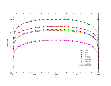
Figure 2: (Color online) $\Pi(l,L)-\alpha l$ for periodic system with total length $L=2000$ with respect to $l$ for different configurations. The dashed lines are the results expected from CFT, i.e. $\frac{1}{16}\ln[\frac{L}{\pi}\sin\frac{\pi l}{L}]+\eta$.

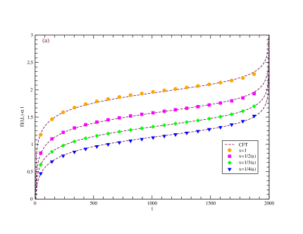
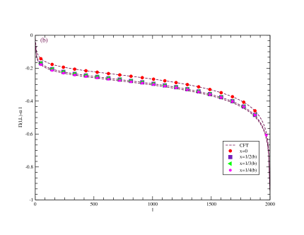
Figure 3: (Color online) $\Pi(l,L)-\alpha l$ for open system with total length $L=2000$ with respect to $l$ for different configurations. a) configurations without boundary changing operators and b) configurations with boundary changing operators. The dashed lines are the results expected from CFT.

We then studied the same configurations for the periodic boundary condition. In the figure  2 it is shown that all of the configurations follow the formula (18) . The case of the open boundary condition is more tricky and depending on the configuration we have two possibilities: When the parity of the number of down spins is independent of the size of the subsystem (for example in the configurations $x=\frac{1}{2}b$ and $\frac{1}{3}b$) we have the formula (19) but when we have the possibility of having odd or even number of down spins in a configurations (for example $x=\frac{1}{2}a,\frac{1}{3}a$) we have the formula (III.1). The results are shown in the Figure  3. This behavior could be anticipated based on the difference between configurations $k=0$ and $k=l$ that we discussed before. It looks like that the boundary changing operator plays a role whenever there is the parity effect in the configuration. Looking to the problem in the language of Euclidean two dimensional classical system one can argue that in the case of open boundary condition we have a strip with a slit on it Stephan2013 . However, the boundary conditions on the boundary of strip can be different from the boundary condition on the slit, consequently, one needs to consider boundary changing operator on the point where the boundary condition changes. However, in general it is not clear which configurations lead to different boundary conditions on the slit and on the boundary of the strip. Our numerical results indeed give a hint that depending on the bahavior of the parity of the number of down spins in a configuration the conformal boundary condition on the slit can be different. In the next two subsections, we will first comment on the validity of the above results in other cases such as non-crystal configurations. Then we will also indicate the possible universal behavior of our results.

IV.1.1 Logarithmic formation probability of non-crystal configurations

The number of crystal configurations is much smaller than the number of the whole configurations. In fact, the number of crystal configurations grows polynomially with the subsystem size but the number of whole configurations grows exponentially. However, numerically it is very simple to check the formula for many configurations that have a small deviation from the crystal states. For example, one can consider the case $k=1$ with all spins up except one and calculate the logarithmic formation probability using the equation (11). It is clear that one does not expect the result be any different from the equation (15) and indeed numerical results confirm this expectation. The important conclusion of this numerical exercise is that there are many configurations ”close” to crystal configurations that indeed follow either the equation (15) or equation (21) with all having the same $\beta$’s but different $\alpha$’s.

The above results strongly suggest that all of the crystal and non-crystal configurations discussed in this section are flowing to some sort of conformal boundary conditions in the scaling limit.

IV.1.2 Universality

To check that the above results are the properties of the Ising universality class we also studied the critical XY-chain which has also central charge $c=\frac{1}{2}$. The Green matrix, in this case, is given by

$$G_{ij}=\int_{0}^{\pi}\frac{d\phi}{\pi}\frac{(\cos\phi-1)\cos[(i-j)\phi]-a\sin\phi\sin\big{[}(i-j)\phi]}{\sqrt{(1-\cos\phi)^{2}+a^{2}\sin^{2}\phi}}.$$

Our numerical results depicted in the Figure  4 show that the coefficient of the logarithmic term is a universal quantity which means that it has a fixed value on the critical XY-line. The coefficient of the linear term changes by varying $a$ which indicates its non-universal nature.

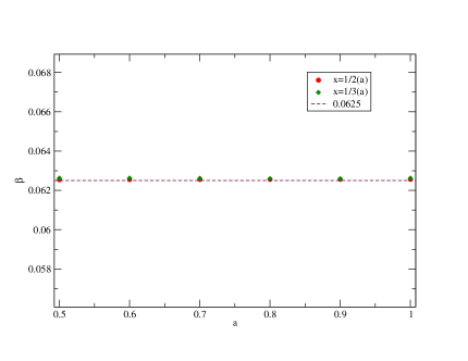
Figure 4: (Color online) The coefficient of the logarithmic term in (15) for two configurations $x=\frac{1}{2}a$ and $x=\frac{1}{3}a$ for different values of $a$. The dashed line is the CFT result. The size of the largest subsystem was $l=500$ and all the results were extracted by fitting the data to $\alpha l+\beta\ln l+\gamma\frac{\ln l}{l}+\nu\frac{(-1)^{m}}{\sqrt{l}}+\delta\frac{1}{l}+\eta$ with suitable $m$ in the range $l\in(100,500)$. Estimated errors in the numerics are in the order of the size of the markers.

IV.2 XX chain

We repeated the calculations of the last section for also critical XX chain. The central charge of the system is $c=1$. The results of logarithmic formation probabilities for different magnetic field $h$ are shown in the Table II and Table III. Based on the numerical calculations we conclude the followings:

1. The configurations with $x=\frac{n_{f}}{\pi}$ follow the equation (15) with $\beta=\frac{1}{8}$. This means that in the scaling limit most probably all of these configurations flow to some sort of bounday conformal conditions. Note that as far as there is no boundary changing operator in the system the equation (15) is valid for any CFT independent of its structure.

2. All the other configurations follow the equation (28) with $\beta$ which is different for different configurations.

As we mentioned earlier XX chain has a $U(1)$ symmetry which means that the number of particles is conserved. The only configurations that respect this symmetry in the subsystem level are the configurations with $x=\frac{n_{f}}{\pi}$. Any injection of the particles into the subsystem changes drastically the formation probability. In the case of $x=0$ this phenomena is already explained in Stephan2013 based on arctic phenomena in the dimer model. It is quite natural to expect that similar structure is valid for all the configurations with $x\neq\frac{n_{f}}{\pi}$. Note that based on our results the coefficient of the $\ln$ is $n_{f}$-dependent and strictly speaking is not a universal quantity.

$n_{f}$	Configuration	$\alpha$	$\beta$
	$x=1/2(a)$	$0.3465735$	$0.124998$
$\pi/2$	$x=1/2(b)$	$0.5198604$	$0.124997$
	$x=1/2(c)$	$0.7127780$	$0.124597$
$\pi/3$	$x=1/3(a)$	$0.3662041$	$0.124987$
$\pi/4$	$x=1/4(a)$	$0.3432345$	$0.125024$

Table 2: Fitting parameters for the logarithmic formation probability of antiferromagnetic configurations with different filling factors. All the results were extracted by fitting the data in the range $l\in(100,300)$ to $\alpha l+\beta\ln l+\gamma\frac{\ln l}{l}+\delta\frac{1}{l}+\eta$.

Configuration	$\alpha_{2}$	$\alpha$	$\beta$
$x=0,1$	$0.346573$	$0.000000$	$0.250054$
$x=1/3(a)$	$0.035191$	$0.366228$	$0.524293$
$x=1/3(b)$	$0.035188$	$0.597663$	$1.578683$
$x=1/4(a)$	$0.080911$	$0.346599$	$0.829767$
$x=1/4(b)$	$0.080910$	$0.587114$	$2.744492$
$x=1/5(a)$	$0.118119$	$0.321924$	$1.144949$
$x=1/6(a)$	$0.147178$	$0.298674$	$1.465399$
$x=1/7(a)$	$0.170072$	$0.278052$	$1.788319$
$x=1/8(a)$	$0.188433$	$0.260021$	$2.112155$
$x=1/9(a)$	$0.203427$	$0.244263$	$2.436061$
$x=1/10(a)$	$0.230432$	$0.230432$	$2.759481$

Table 3: Fitting parameters for different configurations with $x<\frac{1}{2}$ in the XX chain with $n_{f}=\frac{\pi}{2}$. All the data were extracted by fitting the data in the range $l\in(100,300)$ to $\alpha_{2}l^{2}+\alpha l+\beta\ln l+\eta$.

We also studied the finite size effect in this model. The results of the numerical calculations of periodic boundary condition for $x=\frac{1}{2}$ are shown in the Figure  5. It is shown that all of the configurations with $x=\frac{1}{2}$ follow the formula (18) with $c=1$.

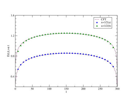
Figure 5: (Color online) $\Pi(l,L)-\alpha l$ for periodic system with total length $L=300$ with respect to $l$ for different configurations for critical $XX$-chain with $n_{f}=\frac{\pi}{2}$. The dashed lines are the results expected from CFT.

We also repeated the same calculations for open boundary conditions. We first performed the calculations for semi-infinite open chain and fitted the results to (15) and extracted the $\beta$. The coefficient of the logarithm not only depends on the rank of the configuration but also to the configuration itself. It also changes with $n_{f}$. We were not able to find any universal feature in this case.

The above results suggest that most probably all of the crystal configurations with $x=\frac{n_{f}}{\pi}$ in the periodic boundary condition flow to a boundary conformal field theory. In the language of Luttinger liquid, the corresponding boundary condition should be the Dirichlet boundary condition Stephan2013 . The case of the open boundary condition is intriguing and we leave it as an open problem.

V Shannon information of a subsystem

In this section, we study Shannon information of a subsystem in transverse-field Ising model and $XX$ chain. For both models, the Shannon information is already calculated in Stephan2014 up to the size $l=40$ which it seems to be the current limit for classical computers. The reason that we are interested in revisiting this quantity is to have a more detailed study of the contribution of different configurations. This will give an interesting insight regarding the possible scaling limit for this quantity.

V.1 Critical Ising

In the last section, we studied many different configurations in the critical Ising model and we found that all of them follow $P_{\mathcal{C}_{n}}=\frac{e^{\alpha_{n}l}}{l^{\frac{c}{8}}}$ with $c=\frac{1}{2}$. The natural expectation is that if we plug this formula in the definition of the Shannon information we get

$$Sh(l)=\alpha l+\frac{c}{8}\ln l+...$$ (29)

where the dots are the subleading terms. The above formula is consistent with AR2013 . However, one should be careful that although there are a lot of crystal configurations (polynomial number of them) and ”close” to crystal configurations that are connected to the central charge it is absolutely not clear what is going to happen in the scaling limit. For example we repeated the calculations of Stephan2014 and realized that extraction of the coefficient of the $\ln$ in the above equation is indeed very difficult, see appendix. Here we show where one should look for the most important configurations. After a bit of inspection and numerical check, one can see that the configuration with the highest probability is the $x=0$. Although the proof of the above statment doesn’t look straightforward one can understand it qualitatively by starting from the ground state of the Ising model with $h\to\infty$ and approaching to the critical point $h=1$. The ground state of the Ising model with $h\to\infty$ is made of a configuration with all spins up. When we decrease the transverse magnetic field the other configurations start to appear in the ground state. Although the amplitude of the configuration with all spins up decreases by decreasing $h$ it still remains always bigger than the other configurations. Another way to look at this phenomena is by looking at the variation of the expectation value of the Hamiltonian $\bar{H}=\langle C|H|C\rangle$ for different configurations $C$. It is easy to see that $\bar{H}$ is minimum for the configuration $C$ with all spins up. This simply means that most probably when one construct the ground state of the Ising model using the variational techniques this configuration playes the most important role. The least important configuration is $x=1$ with the lowest probability. This can also be understood with the same heuristic argument as above. For every rank $k$ of the minors, as we discussed, we have $\binom{l}{k}$ number of configurations which means that for every $x$ for large $l$ we have $e^{f(x)l}$ with $f(x)=-x\ln x-(1-x)\ln(1-x)$ number of configurations. It is obvious that the number of configurations in every rank should be high enough to compensate the exponential decrease of probabilities. We realized that in every rank the configurations a has the lowest probabilities. One can again understand this fact using the variational argument. In this case it is much better to make first the canonical transformation: $\sigma^{x}\to-\sigma^{z}$ and $\sigma^{z}\to\sigma^{x}$ in the Hamiltonian of the crtical Ising model. Then one can simply argue that $\bar{H}$ is big if there are a lot of domain walls, i.e. $\langle C|\sigma_{j}^{z}\sigma_{j+1}^{z}|C\rangle=-1$ in the system which is the case for the configurations a. Other important configurations are the configurations which divide the subsystem to two connected regions with in one part all the spins are up and in the other part all the spins are down. These configurations are interesting because they have the biggest probabilities among all the configurations corresponding to their minor rank. Note that in this case we have just one domain wall. It is not difficult to see that the probability of all of these configurations decay exponentially with the following coefficient $\alpha$:

$$\alpha_{min}(x)=\frac{4C}{\pi}x+\ln 2-\frac{2C}{\pi},$$ (30)

where $C$ is the Catalan constant. In the two extreme points, we recover the previous results. We also checked the validity of the above formula numerically. Having the biggest and smallest probabilities for every rank, we can now easily read the most important ranks. In Figure  6 we depicted the $\alpha_{max}$ and $\alpha_{min}$ for different configurations. We also depicted the graph of the number of configurations in every rank. The Figure clearly show that the configurations with $x>\frac{1}{2}$ can not have any significant contribution in the scaling limit because the number of configurations is not enough to compensate the exponential decay of the probabilities. A similar story seems to be valid also for the values of $x$ close to zero. The reason is that the number of configurations with small $x$ is such low that can not compensate exponential decay of the probabilities in this region to have a significant contribution in the Shannon information. Just the region between the points that the two lines cut each other will most likely survive in the scaling limit.

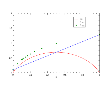
Figure 6: (Color online) Values of $f(x)$, $\alpha_{min}$ and $\alpha_{max}$ with respect to $x$. The red curve is the function $f(x)=-x\log x-(1-x)\ln(1-x)$ and the blue line is the linear function (30). The separated points are the $\alpha_{max}$ regarding the configurations discussed in the text.

The numerical results indeed prove our expectation. In Figure  7 we depicted the contribution of every rank $Sh_{k}(l)$ in Shannon information for two different sizes. As it is quite clear the most important contributions come from $0<x<\frac{1}{2}$. The contribution of the configurations with $x>\frac{1}{2}$ is exponentially small. This means that ignoring a lot of configurations will produce a very small amount of error in the final result of Shannon information. To quantify this argument we calculated the amount of error in the evaluation of the Shannon information if we just keep the configurations with ranks up to $x_{m}$. Suppose $Sh(l,x_{m})$ is the contribution of the configurations with all ranks equal or smaller than $x_{m}$. Then the error of truncation can be calculated by $\mathcal{E}(x_{m},l)=\frac{Sh(l,1)-Sh(l,x_{m})}{Sh(l,1)}$. Interestingly we found that the logarithm of the error function is a linear function of $l$, see Figure  8. In other words

$$\ln\mathcal{E}(x_{m},l)=-\lambda(x_{m})l+\delta(x_{m}),$$ (31)

where $\lambda(x_{m})$ is equal to zero and infinity for $x_{m}=0$ and $x_{m}=1$ respectively. $\lambda(x_{m})$ for the other values are shown in the inset of the Figure  8. The above formula shows that one can calculate Shannon information with a controllable accuracy by ignoring non-important configurations. Although the above truncation method help to calculate the Shannon information with good accuracy (especially the coefficient of the linear term $\alpha$) it is still not good enough to calculate the coefficient of the logarithm with controllable precision.

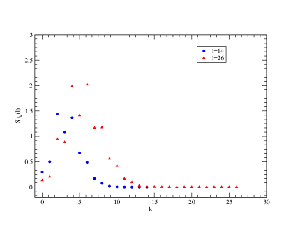
Figure 7: (Color online) The contributions of different ranks $k$ in the Shannon information for two sizes $l=14$ and $26$.

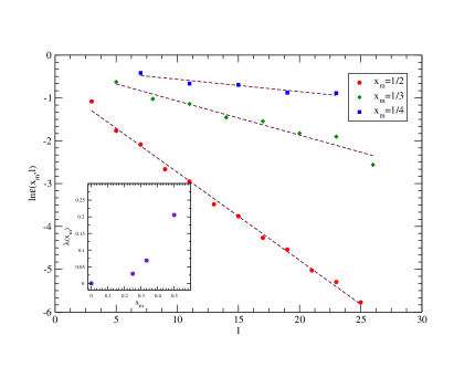
Figure 8: (Color online) The error $\mathcal{E}(x_{m},l)$ in the evaluation of Shannon information coming from the truncation at the rank $k=x_{m}l$. Inset: $-\lambda(x_{m})$ with respect to $x_{m}$.

V.2 XX chain

The Shannon information of the subsystem in the XX-chain is already discussed in Stephan2014 and based on numerical results it is concluded that the equation (30) is valid with $\beta=\frac{1}{8}$ which is consistent with the conjecture in AR2013 . Here we just comment on the contribution of different ranks which shows very different behavior from the transverse field Ising chain case. First of all, as we discussed in the previous section when the external field is zero the only configurations that decay exponentially are those that respect the half filling structure of the total system. The rest of the configurations scale like a Gaussian which simply indicates that their contribution is very small in the Shannon information. This is simply because the number of these configurations scale just exponentially. Based on this simple fact one can anticipate that the only configurations that can survive in the scaling limit are those with $k=\frac{l}{2}$. Numerical results depicted in the Figure  9 indeed support this idea. Although the $k=\frac{l}{2}$ is only one among $l$ possible minor ranks the number of configurations with this rank is highest with respect to the others which can be one of the reasons that one can obtain a good estimate for the coefficient of the logarithm in (30) with relatively modest sizes.

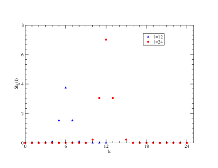
Figure 9: (Color online) The contributions of different ranks $k$ in the Shannon information for two sizes $l=12$ and $24$ in the XX-chain.

VI Evolution of Shannon and mutual information after global quantum quench

Inspired by experimental motivations, the field of quantum non-equilibrium systems has enjoyed a huge boost in the recent decadeexperimental . One of the interesting directions in this field is the study of information propagation after quantum quench, see for example CC-evolution ; Plenio ; LRbound ; fidelity ; Liu ; MM . Based on semiclassical arguments and also using Lieb-Robinson bound it is shown CC-evolution ; LRbound that in one dimensional integrable system one can understand the evolution of entanglement entropy of a subsystem based on quasi-particle picture CC-evolution . The argument is as follows: after the quench, there is an extensive excess in energy which appears as quasiparticles that propagate in time. The quasi-particles emitted from nearby points are entangled and they are responsible for the linear increase of the entanglement entropy of a subsystem with respect to the rest. In this section, we first study the time evolution of formation probabilities and subsequently Shannon and mutual information after a quantum quench. One can consider this section as a complement to the other studies of information propagation after quantum quench. To keep the discussion as simple as possible, we will concentrate on the most simple case of XX-chain or free fermions. Following PeschelEisler consider the Hamiltonian

$$H=-\frac{1}{2}\sum_{m=-\infty}^{+\infty}t_{m}(c_{m}^{\dagger}c_{m+1}+c_{m+1}^{\dagger}c_{m}).$$ (32)

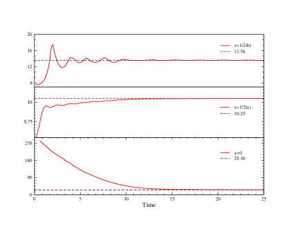
Figure 10: (Color online) The evolution of logarithmic formation probability of different configurations with respect to time $t$ after quantum quench. The size of the subsystem is taken $l=20$.

The time evolution of the correlation functions in the half filling are given as

$$C_{mn}(t)=i^{n-m}\sum_{jl}i^{j-l}J_{m-j}(t)J_{n-l}(t)C_{jl}(0),$$ (33)

where, $J$ is the Bessel function of the first kind. Here we consider the dimerized initial conditions with $t_{2m}=1$ and $t_{2m+1}=0$. The dimerized nature of the initial state will help later to consider different possibilities for the initial Shannon mutual information. Then at time zero we change the Hamiltonian to $t_{m}=1$ and let it evolve. The time evolution of the correlation matrix is given by PeschelEisler

$$C_{mn}(t) = \frac{1}{2}\Big{(}\delta_{m,n}+\frac{1}{2}(\delta_{m+1,n}+\delta_{m-1,n})+e^{-i\frac{\pi}{2}(m+n)}\frac{i(m-n)}{2t}J_{m-n}(2t)\Big{)}.$$ (34)

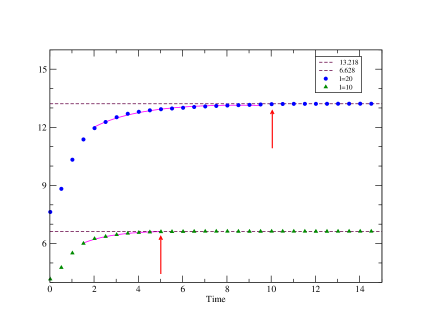
Figure 11: (Color online) The evolution of Shannon information of a subsystem with different sizes with respect to time $t$ after quantum quench. The full lines are the equation (35). The saturation points $t^{*}=\frac{l}{2}$ are marked by vertical arrows.

To calculate the time evolution of the probability of different configurations one just needs to use the above formula in (25). The results for few configurations are shown in the Figure  10. Of course since the sum of all the probabilities should be equal to one some of the probabilities increase with time and some decrease. All the probabilities change rapidly up to time $t^{*}\approx\frac{l}{2}$ and after that saturate. One can also simply calculate the evolution of the Shannon information with the tools of previous sections. In Figure  11 we depicted the evolution of Shannon information of a subsystem with respect to the time $t$. The numerical results show an increase in the Shannon information up to time $t^{*}\approx\frac{l}{2}$ and then saturation. This is similar to what we usually have in the study of the time evolution of von Neumann entanglement entropy after quantum quench CC-evolution . However, one should be careful that in contrast to the von Neumann entropy the Shannon information of the subsystem is not a measure of correlation between the two subsystems. In addition, the increase in the Shannon information of the subsystem is not linear as the evolution of the von Neumann entanglement entropy. Our numerical results indicate that apart from a small regime at the beginning the Shannon information increases as

$$Sh(l)=alt^{b}-dt\hskip 28.45274ptt<t^{*}$$ (35)

where $b\approx 0.15(2)$ and $a$ and $d$ are positive $l$ independent quantities.

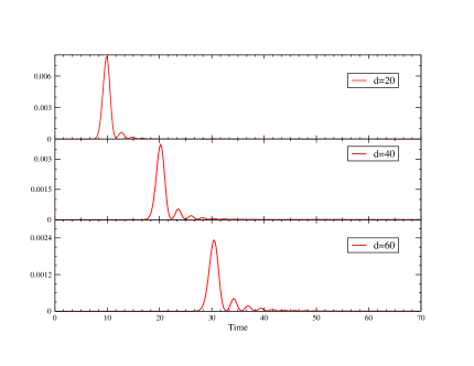
Figure 12: (Color online) The mutual information between a pair of dimers located at distance $d$ with respect to time.

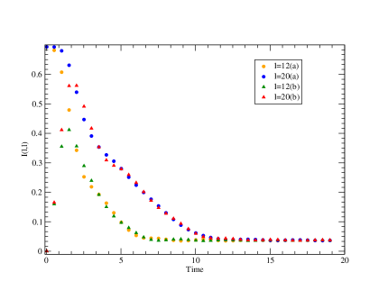
Figure 13: (Color online) The evolution of mutual information between two adjacent subsystems in two different cases: when at the boundary between the two subsystems there is a dimer, case $a$ and when there is no dimer, case $b$. In the first case the mutual information starts from a non-zero value but in the second case it starts from zero.

To study the time evolution of correlations, it is much better to study another quantity, Shannon mutual information of two subsystems. To investigate this quantity we first studied the time evolution of Shannon mutual information of a couple of dimers located far from each other. The results depicted in the Figure  12 show that the Shannon mutual information of the dimers are zero up to time $t^{*}\approx\frac{l}{2}$ and after that increases rapidly and then again decays slowly. This picture is consistent with the quasiparticle picture. The two regions are not correlated up to time that the quasiparticles emitted from the middle point reach each dimerfootnote3 . However, the similarity between the evolution of the von Neumann entropy and mutual Shannon information ends here. To elaborate on that we consider the mutual information of two adjacent regions with sizes $\frac{l}{2}$. Because of the dimerized nature of the initial state there are two possibilities for choosing the subsystems: at time zero at the boundary between the two subsystems there can be a dimer or not. In the first case at time zero the Shannon mutual information between the two subsystems is not zero but in the second case it is zero. In the second case naturally one expects an overall increase in the mutual information but in the first case a priory it is not clear that the mutual information should increase or decrease. In the Figure  13 we have depicted the results of the numerics for the two adjacent subsystems for different sizes. The numerical results show that for the uncorrelated initial conditions the Shannon mutual information first increases rapidly and then it decays and finally saturates at time $t^{*}=\frac{l}{2}$. In the correlated case, we have overall decay in the mutual information and finally the saturation again at time $t^{*}=\frac{l}{2}$. This behavior is very different from the quantum mutual information of the same regions which for the considered initial states first increases linearly and then saturates at time $t^{*}=\frac{l}{2}$. The interesting phenomena is that after a short initial regime that the Shannon mutual information is initial state dependent the system enters to a regime that this quantity is completely independent of initial state and it decreases ”almost” linearly and then saturates. This can be also easily seen from the equation (35), where we can simply drive

$$I(l,l)=-dt\hskip 28.45274ptt<t^{*}.$$ (36)

The saturation regime is independent of the size of the subsystem, this is simply because in the equlibrium regime the Shannon mutual information follows the area-law Wolf2008 and so it is independent of the volume of the subsystems.

VII Conclusions

In this paper, we employed Grassmann numbers to write the probability of occurrence of different configurations in free fermion systems with respect to the minors of a particular matrix. The formula gives a very efficient method to study the scaling properties of logarithmic formation probabilities in the critical XY-chain. In particular, we showed that the logarithmic formation probabilities of crystal configurations are given by the CFT formulas for the critical transverse field Ising model. This is checked by studying the probabilities in the infinite and finite (periodic and open boundary conditions) chain. In the case of critical XX-chain which has a $U(1)$ symmetry just the configurations with $x=\frac{n_{f}}{\pi}$ follow the CFT formulas. The rest of the configurations decay like a Gaussian and do not show much universal behavior. We also studied the Shannon information of a subsystem in the transverse field Ising model and XX-chain. In particular, for the Ising model, we showed that in the scaling limit just the configurations with a high number of up spins contribute to the scaling of the Shannon information. In principle, if one considers all the configurations, with our method one can not calculate the Shannon information with classical computers for sizes bigger than $l=40$ in a reasonable time. However, if one admits a controllable error in the calculation of Shannon information it is possible to hire the results of section V to go to higher sizes. It would be very nice to extend this aspect of our calculations further to calculate the universal quantities in the Shannon information with higher accuracy. For example, one interesting direction can be finding an explicit formula for the sum of different powers of principal minors of a matrix. This kind of formulas can be very useful to calculate analytically or numerically the Rényi entropy of the subsystem.

Finally, we also studied the evolution of formation probabilities after quantum quench in free fermion system. In this case, we prepared the system in the dimer configuration and then we let it evolve with homogeneous Hamiltonian. The evolution of Shannon information of a susbsytem shows a very similar behavior as the evolution of entanglement entropy after a quantum quench. Especially our calculations show that the saturation of the Shannon information of the subsystem occurs at the same time as the entanglement entropy. This is probably not surprising because the $t=t^{*}$ is also the time that the reduced density operator saturates.

It will be very nice to extend our calculations in few other directions. One direction can be investigating the evolution of mutual information after local quantum quenches as it is done extensively in the studies of the entanglement entropy CClocal ; MP ; Karevski . The other interesting direction can be calculating the same quantities in other bases, especially those bases that do not have any direct connection to CFT.

Acknowledgments.

We thank M Fagotti and F Alcaraz for many useful discussions. The work of MAR was supported in part by CNPq. KN acknowledges support from the National Science Foundation under grant number PHY-1314295. MAR also thanks ICTP for hospitality during a period which part of this work was completed.

Appendix A: Shannon information for critical transverse-field Ising model

In this Appendix, we will provide more details regarding the Shannon information of transverse critical Ising chain and XX chain. The data regarding Shannon information for a subsystem with length $l$ up to $l=39$ is listed in the Table A1. Having the data, we checked many different functions with different parameters to study the coefficient of the logarithm. Needless to say increasing the possible parameters can make a difference in the final result. In Stephan2014 the results fitted to

$$Sh(l)=\alpha l+\beta\ln l+\sum_{n=1}^{5}\frac{b_{n}}{l^{n}}+\delta$$ (37)

show that the best value is $\beta=0.060$. This can be also checked using the data provided in the Table A1. It is worth mentioning that one can also get reasonable results using the data up to $l=40$ for some formation probabilities (not all) if we consider extra terms $\sum_{n=1}^{5}\frac{b_{n}}{l^{n}}$ in the fitting procedure. Although we found that the equation (37) is the most stable fit with the least standard deviation based on our results in the main text we found it is hard to exclude the term $\frac{\ln l}{l}$ because it is present in all the configurations studied there. If one includes this term and does not add the terms $\sum_{n=1}^{5}\frac{b_{n}}{l^{n}}$ the $\beta$ coefficient will be $0.0617$. If one keeps all the terms $\sum_{n=1}^{5}\frac{b_{n}}{l^{n}}$ the result will be $\beta=0.060$. The final conclusion is that as far as one justifies the presence of the terms $\sum_{n=1}^{5}\frac{b_{n}}{l^{n}}$ in the Shannon information formula the best value for $\beta$ with the current available data is $0.060$.

l	Shannon	l	Shannon
1	0.473946633733778	21	9.094267377324401
2	0.925441055292197	22	9.520258511384927
3	1.367970612016317	23	9.946131954351737
4	1.805854593071358	24	10.37189747498959
5	2.240889870728481	25	10.79756367448224
6	2.674003797245196	26	11.22313816533366
7	3.105734740754158	27	11.64862771729621
8	3.536422963908594	28	12.07403837729498
9	3.966297046625437	29	12.49937556879184
10	4.395517906953372	30	12.92464417475445
11	4.824203084194648	31	13.34984860684562
12	5.252441034545332	32	13.77499286454422
13	5.473946633733777	33	14.21026702317442
14	6.107833679024358	34	14.62511508430369
15	6.535085171703405	35	15.05009939651494
16	6.962089515106671	36	15.47503630258492
17	7.388875612253789	37	15.89992835887542
18	7.815467577831834	38	16.32477792018708
19	8.241885740227190	39	16.74960160654153
20	8.668147394540807

Table A1: Shannon information calculated for sizes $l=1,2,...,39$.

References

- (1) P. Calabrese, J. Cardy, J. Phys. A 42:504005 (2009)
- (2) V. E. Korepin , A. G. Izergin , F. H. L. Essler and D. B. Uglov , Phys. Lett. A 190 182 (1994) and F. H. L. Essler, H. Frahm, A. G. Izergin and V. E. Korepin, Comm. Math. Phys. 174. 191 (1995)
- (3) N. Kitanine, J-M. Maillet , N. Slavnov and V. Terras, J. Phys. A: Math. Gen 35, L385 (2002); N. Kitanine, J-M. Maillet , N. Slavnov and V. Terras, J. Phys. A: Math. Gen. 35 L753 (2002); A. G. Abanov and V. E. Korepin, Nucl. Phys. B. 647 565 (2002); V. E. Korepin , S. Lukyanov, Y. Nishiyama and M. Shiroishi, Phys. Lett. A 312 21 (2003); K. K. Kozlowski, J. Stat. Mech. P02006 (2008); L. Cantini, J. Phys. A: Math. Theor. 45 135207 (2012)
- (4) M. Shiroishi, M. Takahashi and Y. Nishiyama, J. Phys. Soc. Jpn. 70 3535 (2001)
- (5) A. G. Abanov, F. Franchini, Phys. Lett. A, 316, 342 (2003) and J. Phys. A 38, 5069 (2005)
- (6) J-M Stéphan, J. Stat. Mech. P05010 (2014)
- (7) J-M Stéphan, S. Furukawa, G. Misguich, and V. Pasquier, Phys. Rev. B, 80, 184421 (2009).
- (8) J-M Stéphan, G. Misguich, and V. Pasquier, Phys. Rev. B, 82, 125455 (2010);
- (9) M. Oshikawa [arXiv:1007.3739]
- (10) J-M Stéphan, G. Misguich, and V. Pasquier, Phys. Rev. B 84, 195128 (2011).
- (11) D. J. Luitz, F. Alet, N. Laflorencie, Phys. Rev. Lett. 112, 057203 (2014)
- (12) D. J. Luitz, F. Alet, N. Laflorencie, Phys. Rev. B 89, 165106 (2014)
- (13) D. J. Luitz, N. Laflorencie, F. Alet, J. Stat. Mech. P08007 (2014)
- (14) D. J. Luitz, X. Plat, N. Laflorencie, F. Alet, Phys. Rev. B 90, 125105 (2014)
- (15) M. Hermanns, S. Trebst, Phys. Rev. B 89, 205107 (2014)
- (16) J. Helmes, J-M. Stéphan, S. Trebst, Phys. Rev. B 92, 125144 (2015)
- (17) J. C. Getelina, F. C. Alcaraz, J. A. Hoyos, Phys. Rev. B 93, 045136 (2016)
- (18) M. M. Wolf, F. Verstraete, M. B. Hastings, J. I. Cirac, Phys. Rev. Lett. 100, 070502 (2008).
- (19) J. Wilms, M. Troyer, F. Verstraete, J. Stat. Mech. P10011 (2011)and J. Wilms, J. Vidal, F. Verstraete, S. Dusuel, J. Stat. Mech. P01023 (2012)
- (20) H. W. Lau, P. Grassberger, Phys. Rev. E 87, 022128 (2013)
- (21) O. Cohen, V. Rittenberg, T. Sadhu, J. Phys. A: Math. Theor. 48, 055002 (2015)
- (22) J. Um, H. Park, H. Hinrichsen, J. Stat. Mech. P10026 (2012)
- (23) F. C. Alcaraz, M. A. Rajabpour, Phys. Rev. Lett. 111, 017201 (2013)
- (24) J-M Stéphan, Phys. Rev. B 90, 045424 (2014)
- (25) F. C. Alcaraz, M. A. Rajabpour, Phys. Rev. B, 90, 075132 (2014)
- (26) F. C. Alcaraz, M. A. Rajabpour, Phys. Rev. B, 91, 155122 (2015)
- (27) M. A. Rajabpour, EPL, 112, 66001 (2015)
- (28) M. A. Rajabpour, Phys. Rev. B 92, 075108 (2015)
- (29) M. A. Rajabpour, [arXiv:1512.03940]
- (30) E. Barouch and B. McCoy, Phys. Rev. A 3, 786 (1971)
- (31) M. -C. Chung and I. Peschel, Phys. Rev. B, 62, 4191 (2000) and I. Peschel, J. Phys. A: Math. Gen. 36, L205 (2003)
- (32) T. Barthel, and U. Schollwock, Phys. Rev. Lett. 100, 100601 (2008)
- (33) E. Lieb, T. Schultz, and D. Mattis, Ann. Phys. (NewYork) 16, 407 (1961)
- (34) Similar oscillating behavior exist also in non-critical regime with high transverse magnetic field. In this case the ffect is already understood based on superconducting correlations of real fermions in Franchini .
- (35) M. Fagotti, ”Entanglement and Correlations in exactly solvable models”, unpublished PhD thesis (2011), ETD Università di Pisa.
- (36) Although not shown in the table it is worth mentioning that for those configurations that depending on the parity of the number of down spins we have oscillating behavior the extracted value of is not exactly the same for those cases that is odd or even. However we conjecture that this is just a finite size effect and the formula (21) is correct.
- (37) M. Greiner, O. Mandel, T. W. Hänsch, and I. Bloch, Nature 419, 51 (2002); T. Kinoshita, T. Wenger, D. S. Weiss, Nature 440, 900 (2006); S. Hofferberth, I. Lesanovsky, B. Fischer, T. Schumm, and J. Schmiedmayer, Nature 449, 324 (2007) and S. Trotzky Y.-A. Chen, A. Flesch, I. P. McCulloch, U. Schollwöck, J. Eisert, and I. Bloch, Nature Phys. 8, 325 (2012)
- (38) P. Calabrese, J. Cardy, J. Stat. Mech. P04010 (2005)
- (39) M. B. Plenio, J. Hartley and J. Eisert, New J. Phys. 6, 36 (2004); A. Perales and M. B. Plenio, J. Opt. B: Quantum Semi- class. Opt. 7, S601-S609 (2005); R. G. Unanyan and M. Fleischhauer, Phys. Rev. A 90, 062330 (2014); G. De Chiara, S. Montangero, P. Calabrese and R. Fazio, J. Stat. Mech. 0603, P001 (2006) and M. Fagotti and P. Calabrese 2008 Phys. Rev. A 78 010306 (2008)
- (40) S. Bravyi, M. B. Hastings, and F. Verstraete, Phys. Rev.Lett. 97, 050401 (2006) and J. Eisert, T. J. Osborne, Phys. Rev. Lett. 97, 150404 (2006)
- (41) J. Dubail, J-M Stéphan, J. Stat. Mech. L03002 (2011)
- (42) H. Liu and S. J. Suh, Phys. Rev. Lett. 112, 011601 (2014)
- (43) M. Fagotti, M. Collura, [arXiv:1507.02678]
- (44) V. Eisler and I. Peschel, J. Stat. Mech. P06005 (2007) and J. Phys. A: Math. Theor. 42, 504003 (2009)
- (45) Recently in MM it has been pointed out that because of the presence of integrals of motions instead of two quasiparticles one needs to consider four of them. It is not clear for us how this can change the results of our investigation.
- (46) P. Calabrese, J. Cardy, J. Stat. Mech. P10004 (2007)
- (47) M. Collura, P. Calabrese, J. Phys. A: Math. Theor. 46, 175001 (2013)
- (48) V. Eisler, D. Karevski, T. Platini, I. Peschel, J. Stat. Mech. P01023 (2008)