Unsupervised and Semi-supervised Learning with Categorical Generative Adversarial Networks
Abstract
In this paper we present a method for learning a discriminative classifier from unlabeled or partially labeled data. Our approach is based on an objective function that trades-off mutual information between observed examples and their predicted categorical class distribution, against robustness of the classifier to an adversarial generative model. The resulting algorithm can either be interpreted as a natural generalization of the generative adversarial networks (GAN) framework or as an extension of the regularized information maximization (RIM) framework to robust classification against an optimal adversary. We empirically evaluate our method – which we dub categorical generative adversarial networks (or CatGAN) – on synthetic data as well as on challenging image classification tasks, demonstrating the robustness of the learned classifiers. We further qualitatively assess the fidelity of samples generated by the adversarial generator that is learned alongside the discriminative classifier, and identify links between the CatGAN objective and discriminative clustering algorithms (such as RIM).
1 Introduction
Learning non-linear classifiers from unlabeled or only partially labeled data is a long standing problem in machine learning. The premise behind learning from unlabeled data is that the structure present in the training examples contains information that can be used to infer the unknown labels. That is, in unsupervised learning we assume that the input distribution contains information about – where denotes the unknown label. By utilizing both labeled and unlabeled examples from the data distribution one hopes to learn a representation that captures this shared structure. Such a representation might, subsequently, help classifiers trained using only a few labeled examples to generalize to parts of the data distribution that it would otherwise have no information about. Additionally, unsupervised categorization of data is an often sought-after tool for discovering groups in datasets with unknown class structure.
This task has traditionally been formalized as a cluster assignment problem, for which a large number of well studied algorithms can be employed. These can be separated into two types: (1) generative clustering methods such as Gaussian mixture models, k-means, and density estimation algorithms, which directly try to model the data distribution (or its geometric properties); (2) discriminative clustering methods such as maximum margin clustering (MMC) (Xu et al., 2005) or regularized information maximization (RIM) (Krause et al., 2010), which aim to directly group the unlabeled data into well separated categories through some classification mechanism without explicitly modeling . While the latter methods more directly correspond to our goal of learning class separations (rather than class exemplars or centroids), they can easily overfit to spurious correlations in the data; especially when combined with powerful non-linear classifiers such as neural networks.
More recently, the neural networks community has explored a large variety of methods for unsupervised and semi-supervised learning tasks. These methods typically involve either training a generative model – parameterized, for example, by deep Boltzmann machines (e.g. Salakhutdinov & Hinton (2009), Goodfellow et al. (2013)) or by feed-forward neural networks (e.g. Bengio et al. (2014), Kingma et al. (2014)) –, or training autoencoder networks (e.g. Hinton & Salakhutdinov (2006), Vincent et al. (2008)). Because they model the data distribution explicitly through reconstruction of input examples, all of these models are related to generative clustering methods, and are typically only used for pre-training a classification network. One problem with such reconstruction-based learning methods is that, by construction, they try to learn representations which preserve all information present in the input examples. This goal of perfect reconstruction is often directly opposed to the goal of learning a classifier which is to model and hence to only preserve information necessary to predict the class label (and become invariant to unimportant details)
The idea of the categorical generative adversarial networks (CatGAN) framework that we develop in this paper then is to combine both the generative and the discriminative perspective. In particular, we learn discriminative neural network classifiers that maximize mutual information between the inputs and the labels (as predicted through the conditional distribution ) for a number of unknown categories. To aid these classifiers in their task of discovering categories that generalize well to unseen data, we enforce robustness of the classifier to examples produced by an adversarial generative model, which tries to trick the classifier into accepting bogus input examples.
The rest of the paper is organized as follows: Before introducing our new objective, we briefly review the generative adversarial networks framework in Section 2. We then derive the CatGAN objective as a direct extension of the GAN framework, followed by experiments on synthetic data, MNIST (LeCun et al., 1989) and CIFAR-10 (Krizhevsky & Hinton, 2009).
2 Generative adversarial networks
Recently, Goodfellow et al. (2014) introduced the generative adversarial networks (GAN) framework. They trained generative models through an objective function that implements a two-player zero sum game between a discriminator – a function aiming to tell apart real from fake input data – and a generator – a function that is optimized to generate input data (from noise) that “fools” the discriminator. The “game” that the generator and the discriminator play can then be intuitively described as follows. In each step the generator produces an example from random noise that has the potential to fool the discriminator. The discriminator is then presented a few real data examples, together with the examples produced by the generator, and its task is to classify them as “real” or “fake”. Afterwards, the discriminator is rewarded for correct classifications and the generator for generating examples that did fool the discriminator. Both models are then updated and the next cycle of the game begins.
This process can be formalized as follows. Let be a dataset of provided “real” inputs with dimensionality (i.e. ). Let denote the mentioned discriminative function and denote the generator function. That is, maps random vectors to generated inputs and we assume to predict the probability of example being present in the dataset : . The GAN objective is then given as
| (1) |
where is an arbitrary noise distribution which – without loss of generality – we assume to be the uniform distribution for the remainder of this paper. If both the generator and the discriminator are differentiable functions (such as deep neural networks) then they can be trained by alternating stochastic gradient descent (SGD) steps on the objective functions from Equation (1), effectively implementing the two player game described above.
3 Categorical generative adversarial networks (CatGANs)
Building on the foundations from Section 2 we will now derive the categorical generative adversarial networks (CatGAN) objective for unsupervised and semi-supervised learning. For the derivation we first restrict ourselves to the unsupervised setting, which can be obtained by generalizing the GAN framework to multiple classes – a limitation that we remove by considering semi-supervised learning in Section 3.3. It should be noted that we could have equivalently derived the CatGAN model starting from the perspective of regularized information maximization (RIM) – as described in the appendix – with an equivalent outcome.
3.1 Problem setting
As before, let be a dataset of unlabeled examples. We consider the problem of unsupervisedly learning a discriminative classifier from , such that classifies the data into an a priori chosen number of categories (or classes) . Further, we require to give rise to a conditional probability distribution over categories; that is . The goal of learning then is to train a probabilistic classifier whose class assignments satisfy some goodness of fit measures. Notably, since the true class distribution over examples is not known we have to resort to an intermediary measure for judging classifier performance, rather than just minimizing, e.g., the negative log likelihood. Specifically, we will, in the following, always prefer for which the conditional class distribution for a given example has high certainty and for which the marginal class distribution is close to some prior distribution for all . We will henceforth always assume a uniform prior over classes, that is we expect that the amount of examples per class in is the same for all : 111We discuss the possibility of using different priors in our framework in the appendix of this paper.
A first observation about this problem is that it can naturally be considered as a “soft” or probabilistic cluster assignment task. It could thus, in principle, be solved by probabilistic clustering algorithms such as regularized information maximization (RIM) (Krause et al., 2010), or the related entropy minimization (Grandvalet & Bengio, 2005), or the early work on unsupervised classification with phantom targets by Bridle et al. (1992). All of these methods are prone to overfitting to spurious correlations in the data 222In preliminary experiments we noticed that the MNIST dataset can, for example, be nicely separated into ten classes by creating 2-3 classes for common noise patterns and collapsing together several “real” classes., a problem that we aim to mitigate by pairing the discriminator with an adversarial generative model to whose examples it must become robust. We note in passing, that our method can be understood as a robust extension of RIM – in which the adversary provides an adaptive regularization mechanism. This relationship is made explicit in Section B in the appendix.
A somewhat obvious, yet important, second observation that can be made is that the standard GAN objective cannot directly be used to solve the described problem. The reason for this is that while optimization of Equation (1) does result in a discriminative classifier – which must capture the statistics of the provided input data – this classifier is only useful for determining whether or not a given example belongs to . In principle, we could hope that a classifier which can model the data distribution might also learn a feature representation (e.g. in case of neural networks the hidden representation in the last layer of ) useful for extracting classes in a second step; for example via discriminative clustering. It is, however, instructive to realize that the means by which the function performs the binary classification task – of discriminating real from fake examples – are not restricted in the GAN framework and hence the classifier will focus mainly on input features which are not yet correctly modeled by the generator. In turn, these features need not necessarily align with our concept of classes into which we want to separate the data. They could, in the worst case, be detecting noise in the data that stems from the generator.
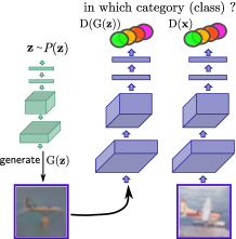
Despite these issues there is a principled, yet simple, way of extending the GAN framework such that the discriminator can be used for multi-class classification. To motivate this, let us consider a change in protocol to the two player game behind the GAN framework (which we will formalize in the next section): Instead of asking to predict the probability of belonging to we can require to assign all examples to one of categories (or classes), while staying uncertain of class assignments for samples from the generative model – which we expect will help make the classifier robust. Analogously, we can change the problem posed to the generator from “generate samples that belong to the dataset” to “generate samples that belong to precisely one out of classes”.
If we succeeded at training such a classifier-generator pair – and simultaneously ensured that the discovered classes coincide with the classification problem we are interested in (e.g. satisfies the goodness of fit criteria outlined above) – we would have a general purpose formulation for training a classifier from unlabeled data.
3.2 CatGAN objective
As outlined above, the optimization problem that we want to solve differs from the standard GAN formulation from Eq. (1) in one key aspect: instead of learning a binary discriminative function, we aim to learn a discriminator that separates the data into categories by assigning a label to each example . Formally, we define the discriminator for this setting as a differentiable function predicting logits for classes: . The probability of example belonging to one of the mutually exclusive classes is then given through a softmax assignment based on the discriminator output:
| (2) |
As in the standard GAN formulation we define the generator to be a function mapping random noise to generated samples :
| (3) |
where again denotes an arbitrary noise distribution. For the purpose of this paper both and are always parameterized as multi-layer neural networks with either linear or sigmoid output.
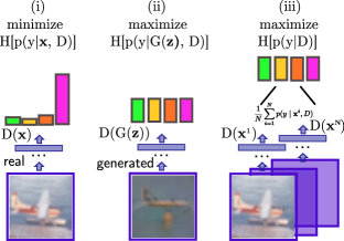
As informally described in Section 3.1, the goodness of fit criteria – in combination with the idea that we want to use a generative model to regularize our classifier – directly dictate three requirements that a learned discriminator should fulfill, and two requirements that the generator should fulfill. We repeat these here before turning them into a learnable objective function (a visualization of the requirements is shown in Figure 1).
Discriminator perspective. The requirements to the discriminator are that it should (i) be certain of class assignment for samples from , (ii) be uncertain of assignment for generated samples, and (iii) use all classes equally 333Since we assume a uniform prior over classes..
Generator perspective. The requirements to the generator are that it should (i) generate samples with highly certain class assignments, and (ii) equally distribute samples across all classes.
We will now address each of these requirements in turn – framing them as maximization or minimization problems of class probabilities – beginning with the perspective of the discriminator. Note that without additional (label) information about the classes we cannot directly specify which class probability should be maximized to meet requirement (i) for any given . We can, nonetheless, formally capture the intuition behind this requirement through information theoretic measures on the predicted class distribution. The most direct measure that can be applied to this problem is the Shannon entropy , which is defined as the expected value of the information carried by a sample from a given distribution. Intuitively, if we want the class distribution conditioned on example to be highly peaked – i.e. should be certain of the class assignment – we want the information content of a sample from it to be low, since any draw from said distribution should almost always result in the same class. If we, on the other hand, want the conditional class distribution to be flat (highly uncertain) for examples that do not belong to – but instead come from the generator – we can maximize the entropy , which, at the optimum, will result in a uniform conditional distribution over classes and fulfill requirement (ii). Concretely, we can define the empirical estimate of the conditional entropy over examples from as
| (4) | ||||
The empirical estimate of the conditional entropy over samples from the generator can be expressed as the expectation of over the prior distribution for the noise vectors , which we can further approximate through Monte-Carlo sampling yielding
| (5) |
and where denotes the number of independently drawn samples (which we simply set equal to ). To meet the third requirement that all classes should be used equally – corresponding to a uniform marginal distribution – we can maximize the entropy of the marginal class distribution as measured empirically based on and samples from :
| (6) | ||||
The second of these entropies can readily be used to define the maximization problem that needs to be satisfied for the requirement (ii) imposed on the generator. Satisfying the condition (i) from the generator perspective then finally amounts to minimizing rather than maximizing Equation (5).
Combining the definition from Equations (4,5,6) we can define the CatGAN objective for the discriminator, which we refer to with , and for the generator, which we refer to with as
| (7) | ||||
where denotes the empirical entropy as defined above and we chose to define the objective for the generator as a minimization problem to make the analogy to Equation (1) apparent. This formulation satisfies all requirements outlined above and has a simple information theoretic interpretation: Taken together the first two terms in are an estimate of the mutual information between the data distribution and the predicted class distribution – which the discriminator wants to maximize while minimizing information it encodes about . Analogously, the first two terms in estimate the mutual information between the distribution of generated samples and the predicted class distribution.
Since we are interested in optimizing the objectives from Equation (7) on large datasets we would like both and to be amenable to to optimization via mini-batch stochastic gradient descent on batches of data – with size – drawn independently from . The conditional entropy terms in Equation (7) both only consist of sums over per example entropies, and can thus trivially be adapted for batch-wise computation. The marginal entropies and , however, contain sums either over the whole dataset or over a large set of samples from within the entropy calculation and therefore cannot be split into “per-batch” terms. If the number of categories that the discriminator needs to predict is much smaller than the batch size , a simple fix to this problem is to estimate the marginal class distributions over the examples in the random mini-batch only: . For we can, similarly, calculate an estimate using samples only – instead of using samples. We note that while this approximation is reasonable for the problems we consider (for which and ) it will be problematic for scenarios in which we expect a large number of categories. In such a setting one would have to estimate the marginal class distribution over multiple batches (or periodically evaluate it on a larger number of examples).
3.3 Extension to semi-supervised learning
We will now consider adapting the formulation from Section 3.2 to the semi-supervised setting. Let be a set of L labeled examples, with label vectors in one-hot encoding, that are provided in addition to the unlabeled examples contained in . These additional examples can be incorporated into the objectives from Equation (7) by calculating a cross-entropy term between the predicted conditional distribution and the true label distribution of examples from (instead of the entropy term used for unlabeled examples). The cross-entropy for a labeled data pair is given as
| (8) |
The semi-supervised CatGAN problem is then given through the two objectives (for the discriminator) and (for the generator) with
| (9) | ||||
where is a cost weighting term and where is the same as in Equation (7): .
3.4 Implementation Details
In our experiments both the generator and the discriminator are always parameterized through neural networks. The details of architectural choices for each considered benchmark are given in the appendix, while we only cover major design choices in this section.
GANs are known to be hard to train due to several unfortunate circumstances. First, the formulation from Equation (1) can become unstable if the discriminator learns too quickly (in which case the loss for the generator saturates). Second, the generator might get stuck generating one mode of the data or it may start wildly switching between generating different modes during training.
We therefore take two measures to stabilize training. First, we use batch normalization (Ioffe & Szegedy, 2015) in all layers of the discriminator and all but the last layer (the layer producing generated examples ) of the generator. This helps bound the activations in each layer and we empirically found it to prevent mode switching of the generator as well as to increase generalization capabilities of the discriminator in the few labels case. Additionally, we regularize the discriminator by applying noise to its hidden layers. While we did find dropout (Hinton et al., 2012) to be effective for this purpose, we found Gaussian noise added to the batch normalized hidden activations to yield slightly better performance. We suspect that this is mainly due to the fact that dropout noise can severely affect mean and variance computation during batch-normalization – whereas Gaussian noise on the activations for which to compute these statistics is a natural assumption.
4 Empirical Evaluation
The results of our empirical evaluation are given in Tables 1, 2 and 3. As can be seen, our method is competitive to the state of the art on almost all datasets. It is only slightly outperformed by the Ladder network utilizing denoising costs in each layer of the neural network.
4.1 Clustering with CatGANs
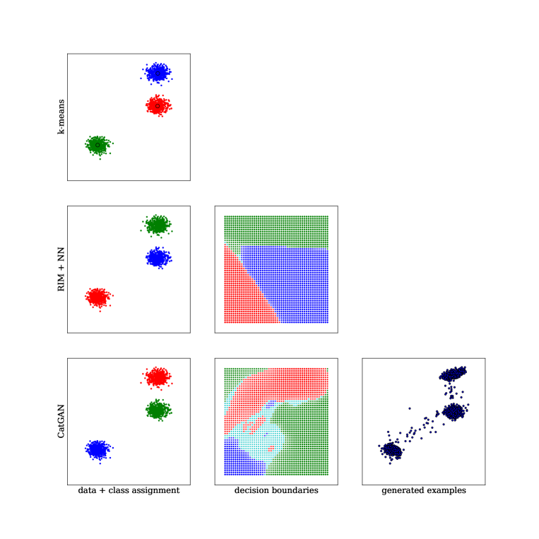
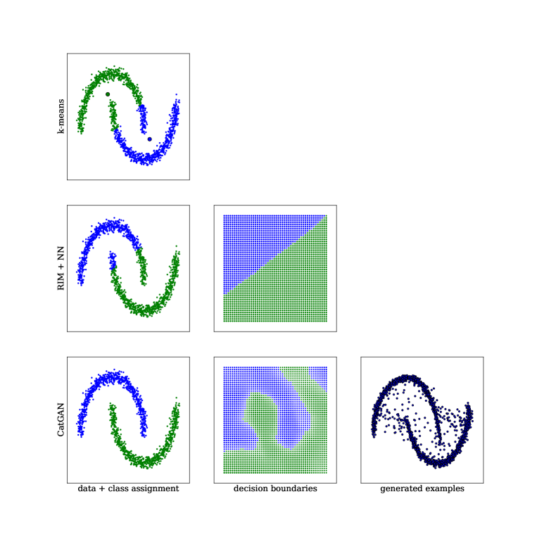
Since categorization of unlabeled data is inherently linked to clustering we performed a first set of experiments on common synthetic datasets that are often used to evaluate clustering algorithms. We compare the CatGAN algorithm with standard k-means clustering and RIM with neural networks as discriminative models, which amounts to removing the generator from the CatGAN model and adding regularization (see Section B in the appendix for an explanation). We considered three standard synthetic datasets – with feature dimensionality two, thus – for which we assumed the optimal number of clusters do be known: the “two moons” dataset (which contains two clusters), the “circles” arrangement (again containing two clusters) and a simple dataset with three isotropic Gaussian blobs of data.
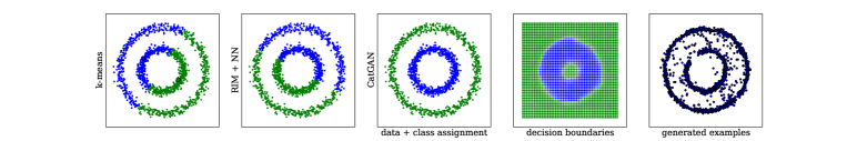
In Figure 2 we show the results of that experiment for the “circles” dataset (plots for the other two experiments are relegated to Figures 4-6 in the appendix due to space constraints). In summary, the simple clustering assignment with three data blobs is solved by all algorithms. For the two more difficult examples both k-means and RIM fail to “correctly” identify the clusters: (1) k-means fails due to the euclidean distance measure it employs to evaluate distances between data points and cluster centers, (2) in RIM the objective function only specifies that the deep network has to separate the data into two equal classes, without any geometric constraints 444We tried to rectify this by adding regularization (we tried both regularization and adding Gaussian noise) but that did not yield any improvement. In the CatGAN model, on the other hand, the discriminator has to place its decision boundaries such that it can easily detect a non-optimal adversarial generator which seems to coincide with the correct cluster assignment. Additionally, the generator quickly learns to generate the datasets in all cases.
| Algorithm | PI-MNIST test error (%) with labeled examples | ||
|---|---|---|---|
| All | |||
| MTC (Rifai et al., 2011) | 12.03 | 100 | 0.81 |
| PEA (Bachman et al., 2014) | 10.79 | 2.33 | 1.08 |
| PEA+ (Bachman et al., 2014) | 5.21 | 2.67 | - |
| VAE+SVM (Kingma et al., 2014) | 11.82 ( 0.25) | 4.24 ( 0.07) | - |
| SS-VAE (Kingma et al., 2014) | 3.33 ( 0.14) | 2.4 ( 0.02) | 0.96 |
| Ladder -model (Rasmus et al., 2015) | 4.34 ( 2.31) | 1.71 ( 0.07) | 0.79 ( 0.05) |
| Ladder full (Rasmus et al., 2015) | 1.13 ( 0.04) | 1.00 ( 0.06) | - |
| RIM + NN | 16.19 ( 3.45) | 10.41 ( 0.89) | |
| GAN + SVM | 28.71 ( 7.41) | 13.21 ( 1.28) | |
| CatGAN (unsupervised) | 9.7 | ||
| CatGAN (semi-supervised) | 1.91 ( 0.1) | 1.73 ( 0.18) | 0.91 |
4.2 Unsupervised and semi-supervised learning of image features
We next evaluate the capabilities of the CatGAN model on two image recognition datasets. We performed experiments using fully connected and convolutional networks on MNIST (LeCun et al., 1989) and CIFAR-10 (Krizhevsky & Hinton, 2009). We either used the full set of labeled examples or a reduced set of labeled examples and kept the remaining examples for semi-supervised or unsupervised learning.
We performed experiments using two setups: (1) using a subset of labeled examples we optimized the semi-supervised objective from Equation (7), and (2) using no labeled examples we optimized the unsupervised objective from Equation (9) with “pseudo” categories. In setup (2) learning was followed by a category matching step. In this second step we simply looked at 100 examples from a validation set (we always kept examples from the training set for validation) for which we assume the correct labeling to be known, and assigned each pseudo category to be indicative of one of the true classes . Specifically we assign to the class for which the count of examples that were classified as and belonged to was maximal. This setup hence bears some similarity to one-shot learning approaches from the literature (see e.g. Fei-Fei et al. (2006) for an application to computer vision). Since no learning is involved in the actual matching step we – somewhat colloquially – refer to this setup as half-shot learning.
The results for the experiment on the permutation invariant MNIST (PI-MNIST) task are listed in Table 1. The table also lists state-of-the-art results for this benchmark as well as two baselines: a version of our algorithm where the generator is removed – but all other pieces stay in place – which we call RIM + NN due to the relationship between our algorithm and RIM; and the discriminator stemming from a standard GAN paired with an SVM trained based on features from it 555Specifically, we first train a generator-discriminator using the standard GAN objective and then extract the last layer features from the discriminator on the available labeled examples, and use them to train an SVM..
While both the RIM and GAN training objectives do produce features that are useful for classifying digits, their performance is far worse than the best published result for this setting. The semi-supervised CatGAN, on the other hand, comes close to the best results, works remarkably well even with only 100 labeled examples, and is only outperformed by the Ladder network with a specially designed denoising objective in each layer. Perhaps more surprisingly the half-shot learning procedure described above results in a classifier that achieves error without the need for any label information during training.
Finally, we performed experiments with convolutional discriminator networks and de-convolutional (Zeiler et al., 2011) generator networks (using the same up-sampling procedure from Dosovitskiy et al. (2015)) on MNIST and CIFAR-10. As before, details on the network architectures are given in the appendix. The results are given in Table 2 and 3 and are qualitatively similar to the PI-MNIST results; notably the unsupervised CatGAN again performs very well, achieving a classification error of . The discriminator trained with the semi-supervised CatGAN objective performed well on both tasks, matching the state of the art on CIFAR-10 with reduced labels.
| Algorithm | MNIST test error (%) with labeled examples | |
|---|---|---|
| All | ||
| EmbedCNN (Weston et al., 2012) | 7.75 | - |
| SWWAE (Zhao et al., 2015) | 8.71 | 0.71 |
| Small-CNN (Rasmus et al., 2015) | 6.43 ( 0.84) | 0.36 |
| Conv-Ladder -model (Rasmus et al., 2015) | 0.86 ( 0.41) | - |
| RIM + CNN | 10.75 ( 2.25) | 0.53 |
| Conv-GAN + SVM | 15.43 ( 1.72) | 9.64 |
| Conv-CatGAN (unsupervised) | 4.27 | |
| Conv-CatGAN (semi-supervised) | 1.39 ( 0.28) | 0.48 |
| Algorithm | CIFAR-10 test error (%) with labeled examples | |
|---|---|---|
| All | ||
| View-Invariant k-means Hui (2013) | 27.4 ( 0.7) | 18.1 |
| Exemplar-CNN (Dosovitskiy et al., 2014) | 23.4 ( 0.2) | 15.7 |
| Conv-Ladder -model (Rasmus et al., 2015) | 20.09 ( 0.46) | 9.27 |
| Conv-CatGAN (semi-supervised) | 19.58 ( 0.58) | 9.38 |
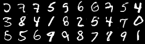
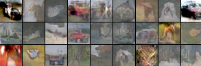
4.3 Evaluation of the generative model
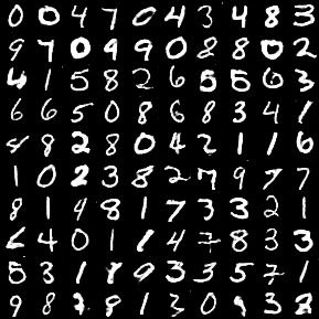
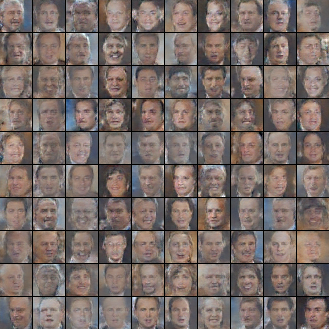
Finally, we qualitatively evaluate the capabilities of the generative model. We trained an unsupervised CatGAN on MNIST, LFW and CIFAR-10 and plot samples generated by these models in Figure 3. As an additional quantitative evaluation we compared the unsupervised CatGAN model trained on MNIST with other generative models based on the log likelihood of generated samples (as measured through a Parzen-window estimator). The full results of this evaluation are given in Table 6 in the appendix. In brief: The CatGAN model performs comparable to the best existing algorithms, achieving a log-likelihood of on MNIST; in comparison, Goodfellow et al. (2014) report for GANs. We note, however, that this does not necessarily mean that the CatGAN model is superior as comparing generative models with respect to log-likelihood measured by a Parzen-window estimate can be misleading (see Theis et al. (2015) for a recent in-depth discussion).
5 Relation to prior work
As highlighted in the introduction our method is related to, and stands on the shoulders of, a large body of literature on unsupervised and semi-supervised category discovery with machine learning methods. While a comprehensive review of these methods is out of the scope for this paper we want to point out a few interesting connections.
First, as already discussed, the idea of minimizing entropy of a classifier on unlabeled data has been considered several times already in the literature (Bridle et al., 1992; Grandvalet & Bengio, 2005; Krause et al., 2010), and our objective function falls back to the regularized information maximization from Krause et al. (2010) when the generator is removed and the classifier is additionally regularized666We note that we did not find regularization to help in our experiments.. Several researchers have recently also reported successes for unsupervised learning with pseudo-tasks, such as self-supervised labeling a set of unlabeled training examples (Lee, 2013), learning to recognize pseudo-classes obtained through data augmentation (Dosovitskiy et al., 2014) and learning with pseudo-ensembles (Bachman et al., 2014), in which a set of models (with shared parameters) are trained such they agree on their predictions, as measured through e.g. cross-entropy. While on first glance these appear only weakly related, they are strongly connected to entropy minimization as, for example, concisely explained in Bachman et al. (2014).
From the generative modeling perspective, our model is a direct descendant of the generative adversarial networks framework (Goodfellow et al., 2014). Several extensions to this framework have been developed recently, including conditioning on a set of variables (Gauthier, 2014; Mirza & Osindero, 2014) and hierarchical generation using Laplacian pyramids (Denton et al., 2015). These are orthogonal to the methods developed in this paper and a combination of, for example, CatGANs with more advanced generator architectures is an interesting avenue for future work.
6 Conclusion
We have presented categorical generative adversarial networks, a framework for robust unsupervised and semi-supervised learning. Our method combines neural network classifiers with an adversarial generative model that regularizes a discriminatively trained classifier. We found the proposed method to yield classification performance that is competitive with state-of-the-art results for semi-supervised learning for image classification and further confirmed that the generator, which is learned alongside the classifier, is capable of generating images of high visual fidelity.
Acknowledgments
The author would like to thank Alexey Dosovitskiy, Alec Radford, Manuel Watter, Joschka Boedecker and Martin Riedmiller for extremely helpful discussions on the contents of this manuscript. Further, huge thanks go to Alec Radford and the developers of Theano (Bergstra et al., 2010; Bastien et al., 2012) and Lasagne (Dieleman et al., 2015) for sharing research code. This work was funded by the the German Research Foundation (DFG) within the priority program “Autonomous learning” (SPP1597).
References
- Bachman et al. (2014) Bachman, Phil, Alsharif, Ouais, and Precup, Doina. Learning with pseudo-ensembles. In Advances in Neural Information Processing Systems (NIPS) 27, pp. 3365–3373. Curran Associates, Inc., 2014.
- Bastien et al. (2012) Bastien, Frédéric, Lamblin, Pascal, Pascanu, Razvan, Bergstra, James, Goodfellow, Ian J., Bergeron, Arnaud, Bouchard, Nicolas, and Bengio, Yoshua. Theano: new features and speed improvements. Deep Learning and Unsupervised Feature Learning NIPS 2012 Workshop, 2012.
- Bengio et al. (2014) Bengio, Yoshua, Thibodeau-Laufer, Eric, and Yosinski, Jason. Deep generative stochastic networks trainable by backprop. In Proceedings of the 31st International Conference on Machine Learning (ICML), 2014.
- Bergstra et al. (2010) Bergstra, James, Breuleux, Olivier, Bastien, Frédéric, Lamblin, Pascal, Pascanu, Razvan, Desjardins, Guillaume, Turian, Joseph, Warde-Farley, David, and Bengio, Yoshua. Theano: a CPU and GPU math expression compiler. In Proceedings of the Python for Scientific Computing Conference (SciPy), 2010.
- Bridle et al. (1992) Bridle, John S., Heading, Anthony J. R., and MacKay, David J. C. Unsupervised classifiers, mutual information and phantom targets. In Advances in Neural Information Processing Systems (NIPS) 4. MIT Press, 1992.
- Denton et al. (2015) Denton, Emily, Chintala, Soumith, Szlam, Arthur, and Fergus, Rob. Deep generative image models using a laplacian pyramid of adversarial networks. In Advances in Neural Information Processing Systems (NIPS) 28, 2015.
- Dieleman et al. (2015) Dieleman, Sander, Schlüter, Jan, Raffel, Colin, Olson, Eben, Sønderby, Søren Kaae, Nouri, Daniel, Maturana, Daniel, Thoma, Martin, Battenberg, Eric, Kelly, Jack, Fauw, Jeffrey De, Heilman, Michael, and et al. Lasagne: First release., August 2015. URL http://dx.doi.org/10.5281/zenodo.27878.
- Dosovitskiy et al. (2015) Dosovitskiy, A., Springenberg, J. T., and Brox, T. Learning to generate chairs with convolutional neural networks. In IEEE Conference on Computer Vision and Pattern Recognition (CVPR), 2015.
- Dosovitskiy et al. (2014) Dosovitskiy, Alexey, Springenberg, Jost Tobias, Riedmiller, Martin, and Brox, Thomas. Discriminative unsupervised feature learning with convolutional neural networks. In Advances in Neural Information Processing Systems (NIPS) 27. Curran Associates, Inc., 2014.
- Ester et al. (1996) Ester, Martin, Kriegel, Hans-Peter, Sander, Jörg, and Xu, Xiaowei. A density-based algorithm for discovering clusters in large spatial databases with noise. In Proc. of 2nd International Conference on Knowledge Discovery and Data Mining (KDD), 1996.
- Fei-Fei et al. (2006) Fei-Fei, L., Fergus, R., and Perona. One-shot learning of object categories. IEEE Transactions on Pattern Analysis Machine Intelligence, 28:594–611, April 2006.
- Funk (2015) Funk, Simon. SMORMS3 - blog entry: RMSprop loses to SMORMS3 - beware the epsilon! http://sifter.org/ simon/journal/20150420.html, 2015.
- Gauthier (2014) Gauthier, Jon. Conditional generative adversarial networks for face generation. Class Project for Stanford CS231N, 2014.
- Goodfellow et al. (2013) Goodfellow, Ian, Mirza, Mehdi, Courville, Aaron, and Bengio, Yoshua. Multi-prediction deep boltzmann machines. In Advances in Neural Information Processing Systems (NIPS) 26. Curran Associates, Inc., 2013.
- Goodfellow et al. (2014) Goodfellow, Ian, Pouget-Abadie, Jean, Mirza, Mehdi, Xu, Bing, Warde-Farley, David, Ozair, Sherjil, Courville, Aaron, and Bengio, Yoshua. Generative adversarial nets. In Advances in Neural Information Processing Systems (NIPS) 27. Curran Associates, Inc., 2014.
- Grandvalet & Bengio (2005) Grandvalet, Yves and Bengio, Yoshua. Semi-supervised learning by entropy minimization. In Advances in Neural Information Processing Systems (NIPS) 17. MIT Press, 2005.
- Hinton & Salakhutdinov (2006) Hinton, G E and Salakhutdinov, R R. Reducing the dimensionality of data with neural networks. Science, 313(5786):504–507, July 2006.
- Hinton et al. (2012) Hinton, Geoffrey E., Srivastava, Nitish, Krizhevsky, Alex, Sutskever, Ilya, and Salakhutdinov, Ruslan R. Improving neural networks by preventing co-adaptation of feature detectors. CoRR, abs/1207.0580v3, 2012. URL http://arxiv.org/abs/1207.0580v3.
- Huang et al. (2007) Huang, Gary B., Ramesh, Manu, Berg, Tamara, and Learned-Miller, Erik. Labeled faces in the wild: A database for studying face recognition in unconstrained environments. Technical Report 07-49, University of Massachusetts, Amherst, October 2007.
- Hui (2013) Hui, Ka Y. Direct modeling of complex invariances for visual object features. In Proceedings of the 30th International Conference on Machine Learning (ICML). JMLR Workshop and Conference Proceedings, 2013.
- Ioffe & Szegedy (2015) Ioffe, Sergey and Szegedy, Christian. Batch normalization: Accelerating deep network training by reducing internal covariate shift. In Proceedings of the 32nd International Conference on Machine Learning (ICML). JMLR Proceedings, 2015.
- Kingma & Ba (2015) Kingma, Diederik and Ba, Jimmy. Adam: A method for stochastic optimization. In International Conference on Learning Representations (ICLR), 2015.
- Kingma et al. (2014) Kingma, Diederik P, Mohamed, Shakir, Jimenez Rezende, Danilo, and Welling, Max. Semi-supervised learning with deep generative models. In Advances in Neural Information Processing Systems (NIPS) 27. Curran Associates, Inc., 2014.
- Krause et al. (2010) Krause, Andreas, Perona, Pietro, and Gomes, Ryan G. Discriminative clustering by regularized information maximization. In Advances in Neural Information Processing Systems (NIPS) 23. MIT Press, 2010.
- Krizhevsky & Hinton (2009) Krizhevsky, A. and Hinton, G. Learning multiple layers of features from tiny images. Master’s thesis, Department of Computer Science, University of Toronto, 2009.
- LeCun et al. (1989) LeCun, Y., Boser, B., Denker, J. S., Henderson, D., Howard, R. E., Hubbard, W., and Jackel, L. D. Backpropagation applied to handwritten zip code recognition. Neural Computation, 1(4):541–551, 1989.
- Lee (2013) Lee, Dong-Hyun. Pseudo-label : The simple and efficient semi-supervised learning method for deep neural networks. In Workshop on Challenges in Representation Learning, ICML, 2013.
- Li et al. (2015) Li, Yujia, Swersky, Kevin, and Zemel, Richard S. Generative moment matching networks. In Proceedings of the 32nd International Conference on Machine Learning (ICML), 2015.
- Mirza & Osindero (2014) Mirza, Mehdi and Osindero, Simon. Conditional generative adversarial nets. CoRR, abs/1411.1784, 2014. URL http://arxiv.org/abs/1411.1784.
- Osendorfer et al. (2014) Osendorfer, Christian, Soyer, Hubert, and van der Smagt, Patrick. Image super-resolution with fast approximate convolutional sparse coding. In ICONIP, Lecture Notes in Computer Science. Springer International Publishing, 2014.
- Rasmus et al. (2015) Rasmus, Antti, Valpola, Harri, Honkala, Mikko, Berglund, Mathias, and Raiko, Tapani. Semi-supervised learning with ladder network. In Advances in Neural Information Processing Systems (NIPS) 28, 2015.
- Rifai et al. (2011) Rifai, Salah, Dauphin, Yann N, Vincent, Pascal, Bengio, Yoshua, and Muller, Xavier. The manifold tangent classifier. In Advances in Neural Information Processing Systems (NIPS) 24. Curran Associates, Inc., 2011.
- Salakhutdinov & Hinton (2009) Salakhutdinov, Ruslan and Hinton, Geoffrey. Deep Boltzmann machines. In Proceedings of the International Conference on Artificial Intelligence and Statistics (AISTATS), 2009.
- Schaul et al. (2013) Schaul, Tom, Zhang, Sixin, and LeCun, Yann. No More Pesky Learning Rates. In International Conference on Machine Learning (ICML), 2013.
- Springenberg et al. (2015) Springenberg, Jost Tobias, Dosovitskiy, Alexey, Brox, Thomas, and Riedmiller, Martin. Striving for simplicity: The all convolutional net. In arXiv:1412.6806, 2015.
- Theis et al. (2015) Theis, Lucas, van den Oord, Aäron, and Bethge, Matthias. A note on the evaluation of generative models. CoRR, abs/1511.01844, 2015. URL http://arxiv.org/abs/1511.01844.
- Tieleman & Hinton (2012) Tieleman, T. and Hinton, G. Lecture 6.5—RmsProp: Divide the gradient by a running average of its recent magnitude. COURSERA: Neural Networks for Machine Learning, 2012.
- Vincent et al. (2008) Vincent, Pascal, Larochelle, Hugo, Bengio, Yoshua, and Manzagol, Pierre-Antoine. Extracting and composing robust features with denoising autoencoders. In Proceedings of the Twenty-fifth International Conference on Machine Learning (ICML), 2008.
- Weston et al. (2012) Weston, J., Ratle, F., Mobahi, H., and Collobert, R. Deep learning via semi-supervised embedding. In Montavon, G., Orr, G., and Muller, K-R. (eds.), Neural Networks: Tricks of the Trade. Springer, 2012.
- Xu et al. (2005) Xu, Linli, Neufeld, James, Larson, Bryce, and Schuurmans, Dale. Maximum margin clustering. In Advances in Neural Information Processing Systems (NIPS) 17. MIT Press, 2005.
- Zeiler et al. (2011) Zeiler, Matthew D., Taylor, Graham W., and Fergus, Rob. Adaptive deconvolutional networks for mid and high level feature learning. In IEEE International Conference on Computer Vision, ICCV, pp. 2018–2025, 2011.
- Zhao et al. (2015) Zhao, Junbo, Mathieu, Michael, Goroshin, Ross, and Lecun, Yann. Stacked what-where auto-encoders. CoRR, abs/1506.02351, 2015. URL http://arxiv.org/abs/1506.02351.
Appendix
Appendix A On the relation between CatGAN and GAN
In this section we will make the relation between the CatGAN objective from Equation (7) in the main paper and the GAN objective given by Equation (1) more directl apparent. Starting from the CatGAN objective let us consider the case . In this case the conditional probabilities should model binary dependent variables (and are thus no longer multinomial). The “correct” choice for the discriminative model is a logistic classifier with output with conditional probability given as . Using this definition The discriminator loss from Equation (7) can be expanded to give
| (10) | ||||
where we introduced the short notation , and dropped the entropy term concerning the empirical class distribution as we only consider one class and hence the classes are equally distributed by definition. Equation (10) now is similar to the GAN objective but pushes the conditional probability for samples from to or and the probability for generated samples towards . To obtain a classifier which predicts we can replace the entropy with the cross-entropy yielding
| (11) | ||||
which is equivalent to the discriminative part of the GAN formulation except for the fact that optimization of Equation (11) will result in examples from the generator being pushed towards the decision boundary of rather than . An equivalent derivation can be made for the generator objective leading to a symmetric objective – just as in the GAN formulation.
Appendix B On the relation between CatGAN and RIM
In this section we re-derive CatGAN as an extension to the RIM framework from Krause et al. (2010). As in the main paper we will restrict ourselves to the unsupervised setting but an extension to the semi-supervised setting is straight-forward. The idea behind RIM is to train a discriminative classifier, which we will suggestively call , from unlabeled data. The objective that is maximized for this purpose is the mutual information between the data distribution and the predicted class labels, which can be formalized as
| (12) |
where the entropy terms are defined as in the main paper and is a regularization term acting on the discriminative model. In Krause et al. (2010) was chosen as a logistic regression classifier and consisted of regularization on the discriminator weights. If we instantiate to be a neural network we obtain the baseline RIM + NN which we considered in our experiments.
To connect the RIM objective to the CatGAN formulation from Equation (7) we can set let , that is we let measure the negative entropy of samples from the generator. With this setting we achieve equivalence between and . If we now also train the generator alongside the discriminator using the objective we arrive at the CatGAN formulation.
Appendix C On different priors for the empirical class distribution
In the main paper we always assumed a uniform prior over classes, that is we enforced that the amount of examples per class in is the same for all : . This was achieved by maximizing the entropy of the class distribution . If this prior assumption is not valid our method could be extended to different prior distributions similar to how RIM can be adapted (see Section 5.2 of Krause et al. (2010)). This becomes easy to see ny noticing the relationship between the Entropy and the KL divergence: where denotes the discrete uniform distribution. We can thus simply drop the constant term and use directly, allowing us to replace with an arbitrary prior – as long as we can differentiate through the computation of the KL divergence (or estimate it via sampling).
Appendix D Detailed explanation of the training procedure
As mentioned in the main Paper we perform training by alternating optimization steps on and . More specifically, we use batch size in all experiments and approximate the expectations in Equation (7) and Equation (9) using random examples from , and the generator respectively. We then do one gradient ascent step on the objective for the discriminator followed by one gradient descent step on the objective for the generator. We also added noise to all layers as mentioned in the main paper. Since adding noise to the network can result in instabilities in the computation of the entropy terms from our objective (due to small values inside the logarithms which are multiplied with non-negative probabilities) we added noise only to the terms not appearing inside logarithms. That is we effectively replace with the cross-entropy , where is the network with added noise and additionally truncate probabilities to be bigger than . During our evaluation we experimented with Adam (Kingma & Ba, 2015) for adapting learning rates but settled for a hybrid between (Schaul et al., 2013) and rmsprop (Tieleman & Hinton, 2012), called SMORMS3 (Funk, 2015) which we found slightly easier to use as it only has one free parameter – a maximum learning rate – which we did always set to .
D.1 Details on network architectures
D.1.1 Synthetic benchmarks
For the synthetic benchmarks we used neural networks with three hidden layers, containing 100 leaky rectified linear units each (leak rate ), both for the discriminator and the generator (where applicable). Batch normalization was used in all layers (with added Gaussian noise with standard deviation ) and the dimensionality of the noise vectors for the CatGAN model was chosen to be for. Note that while such large networks are most certainly an “overkill” for the considered benchmarks, we did chose these settings to ensure that learning was easily possible. We also experimented with smaller networks but did not find them to result in better decision boundaries or more stable learning.
| Model | |
|---|---|
| discriminator | generator |
| Input Gray image | Input |
| conv. lReLU | fc lReLU |
| max-pool, stride | perforated up-sampling |
| conv. lReLU | conv. lReLU |
| conv. lReLU | |
| max-pool, stride | perforated up-sampling |
| conv. lReLU | conv. lReLU |
| conv. lReLU | conv. lReLU |
| fc lReLU | |
| 10-way softmax | |
| Model | |
|---|---|
| generator | discriminator |
| Input RGB image | Input |
| conv. lReLU | fc lReLU |
| conv. lReLU | |
| conv. lReLU | |
| max-pool, stride | perforated up-sampling |
| conv. lReLU | conv. lReLU |
| conv. lReLU | conv. lReLU |
| conv. lReLU | |
| max-pool, stride | perforated up-sampling |
| conv. lReLU | conv. lReLU |
| conv. lReLU | |
| conv. lReLU | conv. lReLU |
| global average | |
| 10-way softmax | |
D.1.2 Permutation invariant MNIST
For the permutation invariant MNIST task we used fully connected generator and discriminator networks with leaky rectified linearities (and a leak rate of ). For the discriminator we used the same architecture as in Rasmus et al. (2015), consisting of a network with 5 hidden layers (with sizes 1000, 500, 250, 250, 250 respectively). Batch normalization was applied to each of these layers and Gaussian noise was added to the batch normalized responses as well as the pixels of the input images (with a standard deviation of 0.3). The generator for this task consisted of a network with three hidden layers (with hidden sizes 500, 500, 1000) respectively. The output of this network was of size , producing pixel images, and used a sigmoid nonlinearity. The noise dimensionality for vectors was chosen as and the cost weighting factor was simply set to . Note that on MNIST the classifier quickly learns to classify the few labeled examples leading to a vanishing supervised cost term; in a sense the labeled examples serve more as a “class initialization” in these experiments. We note that we found many different architectures to work well for this benchmark and merely settled on the described settings to keep our results somewhat comparable to the results from Rasmus et al. (2015).
D.1.3 CNNs for MNIST and CIFAR-10
Full details regarding the CNN architectures used both for the generator and the discriminator are given in Table 4 for MNIST and in Table 5 for CIFAR-10. They are similar to the models from Rasmus et al. (2015) who, in turn, derived them from the best models found by Springenberg et al. (2015). In the Table ReLU denotes rectified linear units, lReLU denotes leaky rectified linear units (with leak rate 0.1), fc stands for a fully connected layer, conv for a convolutional layer and perforated up-sampling denotes the deconvolution approach derived in Dosovitskiy et al. (2015) and Osendorfer et al. (2014).
Appendix E Additional experiments
E.1 Quantitative evaluation of the generative model
Table 6 shows the sample log-likelihood for samples from an unsupervised CatGAN model. The CatGAN model performs comparable to the best existing algorithms; except for GMMN + AE which does not generate images directly but generates hidden layer activations of an AE that then reconstructs an image. As noted in the main paper we however want to caution the reader comparing generative models with respect to log-likelihood as measured by a Parzen-window estimate can be misleading (see Theis et al. (2015) for a recent in-depth discussion).
E.2 Additional plots for experiments on synthetic data
In Figure 4, 4 and 6 we show the results of training k-means, RIM and CatGAN models on the three synthetic datasets from the main paper. Only the CatGAN model “correctly” clusters the data and, as an aside, also produces a generative model capable of generating data points that are almost indistinguishable from those present in the dataset. It should be mentioned that there exist clustering algorithms – such as DBSCAN (Ester et al., 1996) or spectral clustering methods – which can correctly identify the clusters in the datasets by making additional assumptions on the data distribution.
E.3 Additional visualizations of samples from the generative model
We depict additional samples from an unsupervised CatGAN model trained on MNIST and Labeled Faces in the Wild (LFW)(Huang et al., 2007) in Figures 7 and 8. The architecture for the MNIST model is the same as in the semi-supervised experiments and the architecture for LFW is the same as for the CIFAR-10 experiments.