GeMs/GSAOI observations of La Serena 94: an old and far open cluster inside the solar circle

Abstract

Physical properties were derived for the candidate open cluster La Serena 94, recently unveiled by the VVV collaboration. Thanks to the exquisite angular resolution provided by GeMS/GSAOI, we could characterize this system in detail, for the first time, with deep photometry in $JHK_{\rm s}$–bands. Decontaminated $JHK_{\rm s}$ diagrams reach about 5 mag below the cluster turnoff in $H$. The locus of red clump giants in the colour–colour diagram, together with an extinction law, was used to obtain an average extinction of $A_{V}=14.18\pm 0.71$. The same stars were considered as standard–candles to derive the cluster distance, $8.5\pm 1.0$ kpc. Isochrones were matched to the cluster colour–magnitude diagrams to determine its age, $\log{t({\rm yr})}=9.12\pm 0.06$, and metallicity, $Z=0.02\pm 0.01$. A core radius of $r_{\rm c}=0.51\pm 0.04$ pc was found by fitting King models to the radial density profile. By adding up the visible stellar mass to an extrapolated mass function, the cluster mass was estimated as $\mathcal{M}=(2.65\pm 0.57)\times 10^{3}$ M_⊙, consistent with an integrated magnitude of $M_{K_{\rm s}}=-5.82\pm 0.16$ and a tidal radius of $r_{\rm t}=17.2\pm 2.1$ pc. The overall characteristics of La Serena 94 confirm that it is an old open cluster located in the Crux spiral arm towards the fourth Galactic quadrant and distant $7.30\pm 0.49$ kpc from the Galactic centre. The cluster distorted structure, mass segregation and age indicate that it is a dynamically evolved stellar system.

1 Introduction

Galactic open clusters are key to the development of the theories on formation and evolution of galaxies. Indeed, in the last decades the studies of Galactic clusters have proven to be extremely important astrophysical laboratories for a wide range of problematic issues, particularly those pertaining to the disc abundance gradients and age–metallicity relations (Piatti, Clariá & Abadi 1995; Carraro, Ng & Portinari 1998; Hou, Chang & Chen 2002; Magrini et al. 2015). The knowledge and accurate measurement of clusters’ fundamental parameters like age, heliocentric distance, reddening, metallicity, mass and size, play a key role in studies of the Milky Way (MW) global properties, such as its formation history (Friel 1995) and dynamical properties (Dias & Lépine 2005). In this sense, the study of the stellar populations of old open clusters may contribute to answer some fundamental questions related to the structure and evolution of the Galaxy during its early formation time (Barbaro & Pigatto 1984; van den Bergh 1996; De Silva, Freeman & Bland-Hawthorn 2009, and references therein).

In one hand, the study of old open clusters in the Galactic plane, particularly those situated towards the first and fourth quadrants inside the solar circle, is problematic due to the high and patchy extinction, which makes optical observations difficult to impossible along most lines of sight. Also, crowding may be a limitation, mainly in directions where more than one spiral arm may be present. With the advent of deep near–infrared surveys like 2MASS (Skrutskie 2006), VVV (Minniti et al. 2010), and WISE (Wright et al. 2010), hundreds of new cluster candidates have been found in the past years (Dutra & Bica 2001; Ivanov et al. 2002; Kronberger et al. 2006; Borissova et al. 2014; Barbá et al. 2015; Camargo, Bica & Bonatto 2015), making possible further study of new old open cluster candidates placed inside or near the solar circle (Friel 1995; Bonatto et al. 2010). On the other hand, open clusters older than $\sim$1 Gyr are normally found near the solar circle and/or in the outer Galaxy (Friel 1995), where dynamical interactions with giant molecular clouds and the disk is less common (Salaris, Weiss & Percival 2004).

Adaptive optics systems are especially useful to the investigation of relatively compact, obscured and distant star clusters in the Galactic disc (Momany et al. 2008). We present a study of La Serena 94 (hereafter LS 94), localized in the fourth Galactic quadrant. The object is one of the star cluster candidates detected in the VISTA Variables in the Vía Láctea ESO public survey by Barbá et al. (2015). The present study is based on high spatial resolution, near–infrared images obtained with the first Multi–Conjugate Adaptive Optics system in use in a 8–m telescope.

The paper is organized as follows. In Section 2 we describe the observations and data reduction, including the point spread function analysis and the photometric calibration of the stars detected in the observed field. The centre determination and the stellar density map of the cluster candidate are presented in Section 3. Section 4 contains a detailed analysis of LS 94 stellar population concerning its radial variation and the determination of photometric membership from decontaminated photometry. In Section 5, the cluster fundamental parameters reddening, distance, age and metallicity are derived. An investigation of the structural properties and their consequences is presented in Section 6. Section 7 shows the luminosity and mass functions, built to derive the cluster overall luminosity and mass, from which the tidal radius is estimated. The results are discussed in Section 8 and the conclusions given in Section 9.

2 Data acquisition and reductions

2.1 Observations

The observations of LS 94 were obtained with the Gemini–South telescope using the Gemini South Adaptive Optics Imager (GSAOI – McGregor et al. 2004; Carrasco et al. 2012) and the Gemini South Multi–Conjugate Adaptive Optics System (GeMS – Rigaut et al. 2014; Neichel et al. 2014a). GeMS is a facility Adaptive Optics (AO) system for the Gemini South telescope. This AO system uses five sodium Laser Guide Stars (LGSs) to correct for atmospheric distortion and up to three Natural Guide Stars (NGSs) brighter than $R=15.5$ mag to compensate for tip–tilt and plate modes variation over a 2 arcmin  field–of–view (FoV) of the AO bench unit (CANOPUS, Rigaut et al. 2014). GSAOI is a near–infrared AO camera used with GeMS. Together, the two facility instruments can deliver near–diffraction limited images in the wavelength interval of 0.9 – 2.4$\micron$. The GSAOI detector is formed by $2\times 2$ mosaic Rockwell HAWAII-2RG $2048\times 2048$ arrays. At the f/32 GeMS output focus, GSAOI provides a FoV of 85 $\times$ 85 arcsec² on the sky with a 0.02 arcsec per pixel sampling and gaps of $\sim 3$ arcsec between arrays.

The cluster LS 94 was imaged through the $J$ (1.250 $\micron$), $H$ (1.635 $\micron$) and $K$ (2.200 $\micron$) filters during the night of May 22 – 23, 2013, as part of the program GS-2012B-SV-499 (GeMS/GSAOI commissioning data ). For each filter, 9 images of 60 seconds were obtained, providing an effective exposure time of 540 seconds. An offset of 4 arcsec between individual images, following a $3\times 3$ dither pattern, was used to fill the gaps between arrays. Because LS 94 is located in a crowded sky region in the Galactic plane, sky frames were observed in a separate region located 10 degrees North of the position of the cluster centre using the same dither pattern and offset size as the main target. The images were obtained under photometric conditions and variable seeing. The values for the natural seeing from the DIMM monitor at Cerro Pachón, the average resolution derived from stars over the field per filter (AO FWHM, see Sec. 2.3) and the average Strehl ratios are shown in Table 1.

Table 1: Observing log

Filter	Exp. Time	Airmass	Seeing	AO FWHM	Strehl
	[s]		[arcsec]	[mas]	Ratio [%]
$K$	$9\times 60$	1.202	0.79$\pm$0.10	98$\pm$13	$12\pm 2$
$H$	$9\times 60$	1.212	0.84$\pm$0.12	102$\pm$15	$9\pm 2$
$J$	$9\times 60$	1.223	1.03$\pm$0.22	211$\pm$22	$3\pm 2$

2.2 Data reduction

The data were reduced following the standard procedures for near–infrared imaging provided by the Gemini/GSAOI package inside IRAF (Tody 1986). Each science image was processed with the program GAREDUCE. The arrays in the science frames were corrected for non–linearity, subtracted off the sky, divided by the master domeflat fields image, and multiplied by the GAIN to convert from ADU to electrons.

Prior to mosaic the science frames and create images with a single extension, it is necessary to remove the instrumental distortion produced by the off-axis parabolic system used in GeMS (Rigaut et al. 2012, 2014). The instrumental distortion was corrected using a high–order distortion map derived from an astrometric field located in the Large Magellanic Cloud. The positions of the stars in this field were derived from the HST/ACS data (HST Proposal 10753, PI: Rosa Diaz-Miller, Cycle 14). The distortion map was derived using the position of about 300 stars uniformly distributed across the GSAOI detector. The distortion map has a star–position accuracy less than $\sim$ 0.1 arcsec. We used the program MSCSETWCS inside the MSCRED package to apply the distortion correction to each GSAOI array. The program MSCIMAGE was employed to resample each GSAOI multi–extension frame into a single image and to a common reference position.

Unfortunately, the distortion correction applied above does not remove all the instrumental distortion. There is a dynamic distortion component (see Rigaut et al. 2012; Neichel et al. 2014b) which depend on the location of the NGSs in the GeMS patrol field, the size of the offsets and the dither pattern used. This effect is more pronounced in the outer parts of the mosaic–ed images where the position of a given star in the different images can have variations of up to 10 pixels. Moreover, given the spatial resolution of our GeMS/GSAOI images, in particular for the $K$–band (see Table 1), this effect has to be corrected, otherwise the co–addition will be wrong. To correct the dynamic distortion and co–add the images, we have used a modified version of the IMCOADD program inside the GEMINI/GEMTOOLS package. For each filter, the first image is used as a reference to search for stars using the NOAO/DAOFIND program. Then, a geometrical transformation is derived to register the images to a common pixel position using unsaturated stars in common between the images with the GEOMAP program. The derived transformation is applied to each image with the GEOTRANS program. Lastly, the images are combined by averaging the good pixels. The rms of the resulting fit in the individual images was less than 0.1 pixels.

The WCS in the final co–added images need to be calibrated in order to have all filters registered to a common WCS and pixel positions. The WCS was calibrated using a catalogue of non–saturated stars derived from the VIRCAM/VVV $K_{\rm s}$ image and uniformly distributed across the GSAOI FoV. We used the CCMAP program to derive a linear transformation (translation, scale and rotation) to correct the WCS in all co–added images. The final co–added images have an accuracy in the WCS solution (average astrometric error) of $\sim$ 0.05 arcsec. Fig. 1 shows the $JHK$ colour composite image of LS 94. The big circle indicates the location of the cluster candidate. The positions of the NGSs are depicted. The corrected AO FWHM and Strehl ratios derived from the final co–added images are presented in Table 1.

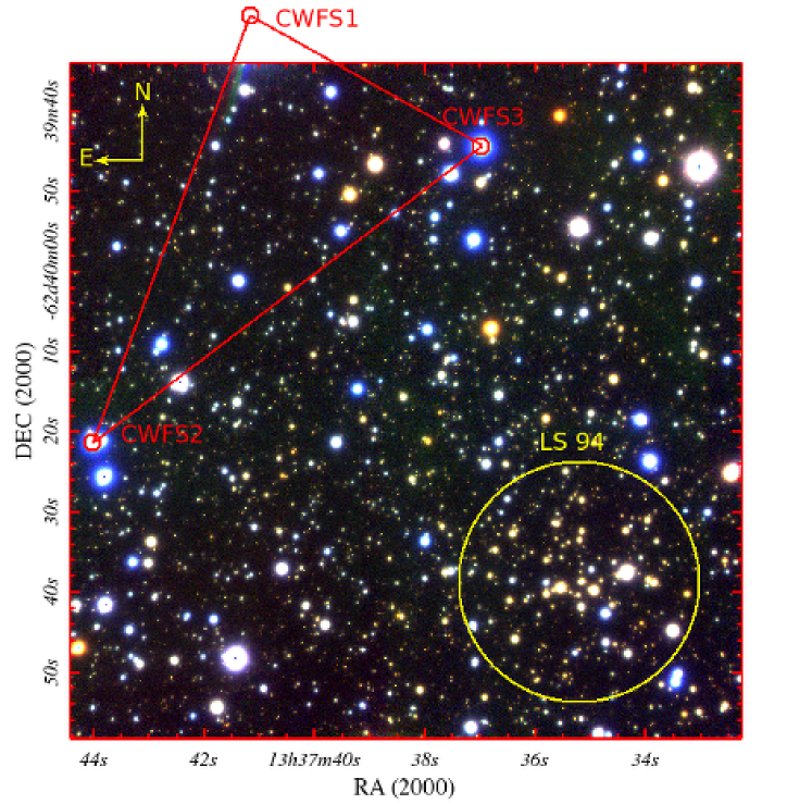
Figure 1: $J$ (blue), $H$ (green), $K$ (red) colour composite image of LS 94. The yellow circle (30 arcsec of diameter) indicates the position of the cluster candidate. The red small circles show the location of the natural guide stars used during the observations. The size of the image is 85$\times$85 arcsec².

2.3 Photometry

The program starfinder (Diolaiti et al. 2000) was used to perform point spread function (PSF) photometry. The PSF model was built from several (typically 40) relatively bright, isolated stars uniformly distributed across the frames. Isoplanatism was evaluated for the pre–reduced, combined images using IRAF task psfmeasure. Fig. 2 gives information on the spatial variation of the delivered image quality of randomly located stars in the $K$ frame. These stars were used to built the average PSF employed in the photometric reduction. Fig. 2 shows also how the stellar profile parameters FWHM and ellipticity vary along lines and columns of the detector. The circle sizes indicate the observed FWHM (blue if it is above the average and red if it is below the average), and the asterisk sizes indicate the relative magnitude of the stars. There is an evident tendency for smaller FWHM and ellipticities to lie in the superior part of the frame, where the NGS are located and, in consequence, the AO correction performed better. However, the difference towards opposite sides of the frame are small, as reflected by the dispersion of the FWHM, $0.098\pm 0.013$ arcsec.

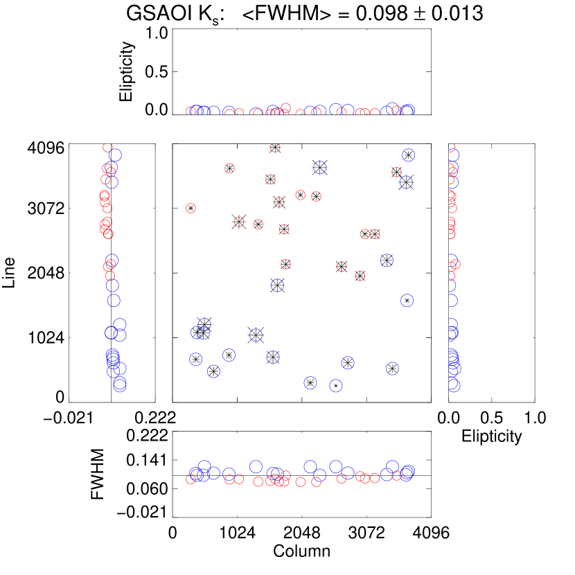
Figure 2: Spatial variation of the PSF for the GSAOI $K$ combined image, with the FWHM values given in arcsec. Asterisk sizes indicate the magnitude of the stars while circle sizes represent the FWHM of the stars, which is blue if above the average and red if below the average.

The same analysis was performed for the $J$ and $H$ combined frames. Although there is a degradation of the image quality compared to the $K$ band, as expected for shorter wavelengths, it is minor. The anisoplanatism is even less noticeable for $J$ and $H$ than for $K$. The FWHM is $0.211\pm 0.022$ arcsec and $0.102\pm 0.015$ arcsec for $J$ and $H$, respectively.

The extinction coefficients ($k_{J}=0.015$, $k_{H}=0.015$, $k_{K}=0.033$) and an initial zeropoint (25.0 mag) were adopted to transform the PSF flux into instrumental magnitudes, which were calibrated to the 2MASS photometric system. With this aim, we resort to the VISTA Variables in the Vía Láctea (VVV) survey (Minniti et al. 2010; Saito et al. 2010), which collected near–infrared photometry of selected regions of our Galaxy disc and bulge with the VISTA 4–m telescope (Visible and Infrared Survey Telescope for Astronomy). Specifically, the positions of stars in the VVV photometry in common with the GSAOI FoV were matched and the instrumental magnitudes from GSAOI calibrated against VVV magnitudes (in the 2MASS photometric system).

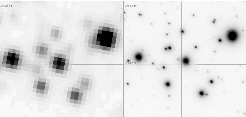
Figure 3: VVV $K_{\rm s}$ (left) and GSAOI $K$ (right) images are compared for the cluster core region. Each frame is $12\times 13$ arcsec². North is to the top and East to the left.

Fig. 3 contrasts VVV $K_{\rm s}$ and GSAOI $K$ images of the central regions of the cluster evidencing the improvement of spatial resolution and photometric deepness of GSAOI over VVV. The difference between the VVV magnitude and the GSAOI (instrumental) magnitude for $JH$ filters is shown in Fig. 4. The same difference is shown for the $K$ band, but it refers to the 2MASS $K_{\rm s}$ (2.150 $\micron$) in the case of VVV magnitudes. For all bands, the data distribution could be fit by a zero-order polynomium (constant), except where stars are saturated (only in the $K$–band) or affected by unresolved binaries and crowding in VVV data. Therefore, a constant was fit to selected magnitude ranges excluding these stars (darker symbols in Fig. 4). The straight line represents the average weighted by the magnitude uncertainties, mathematically:

$$J(VVV)-J(GSAOI)=1.69530\pm 0.00089$$ (1)

$$H(VVV)-H(GSAOI)=1.92705\pm 0.00070$$ (2)

$$K_{\rm s}(VVV)-K(GSAOI)=1.3393\pm 0.0015$$ (3)

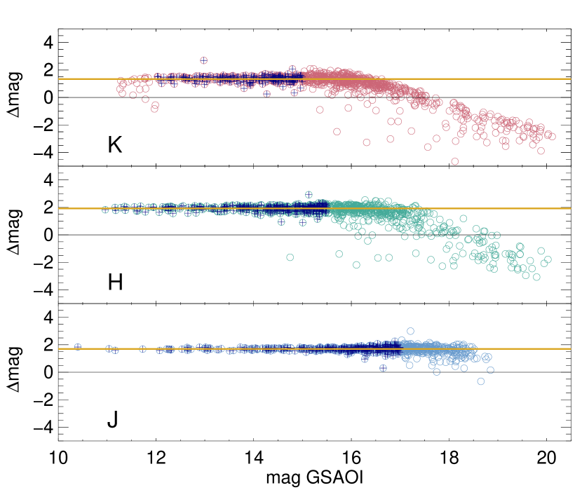
Figure 4: The difference between the VVV magnitude and the GSAOI (instrumental) magnitudes. A constant (straight line) was fit to selected ranges of magnitude (plusses) excluding stars affected by saturation, unresolved binaries and crowding.

The final magnitude uncertainties were obtained by propagation considering the above calibration errors and the PSF errors. Magnitudes of GSAOI saturated stars were replaced by 2MASS magnitudes. This procedure only affects stars with $K<12.0$. Fig. 5 shows the final magnitude errors of GSAOI data compared to data from 2MASS and VVV in the field of GSAOI. The same is presented in Fig. 6 for the CMD $K_{\rm s}$ vs $H-K_{\rm s}$, where the uncertainties of GSAOI photometry are indicated by error bars. Along the Galactic disc, we expect a rising number of stars as the magnitude increases, until source confusion associated to the instrumental sensitivity cause this number to drop making the data no longer complete. Fig. 7 shows this trend, where the magnitude for which the star counts peak indicates the estimated $\sim 100\%$ completeness limits of 19.3, 21.2 and 20.7 magnitudes for $J$, $H$ and $K_{\rm s}$, respectively.

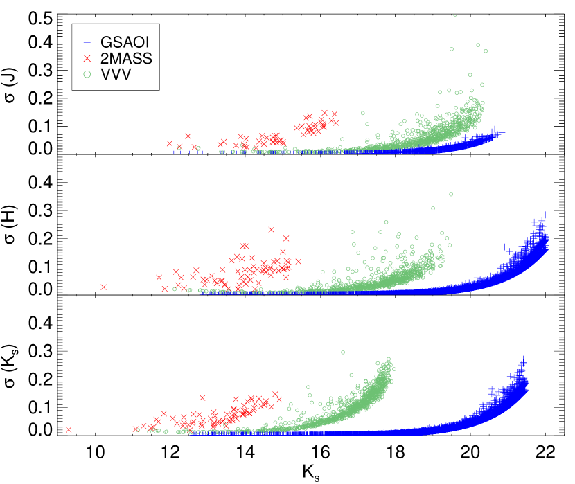
Figure 5: Uncertainties in $J$, $H$ and $K_{\rm s}$ for 2MASS (red crosses), VVV (green circles) and GSAOI (blue plusses) data compared.

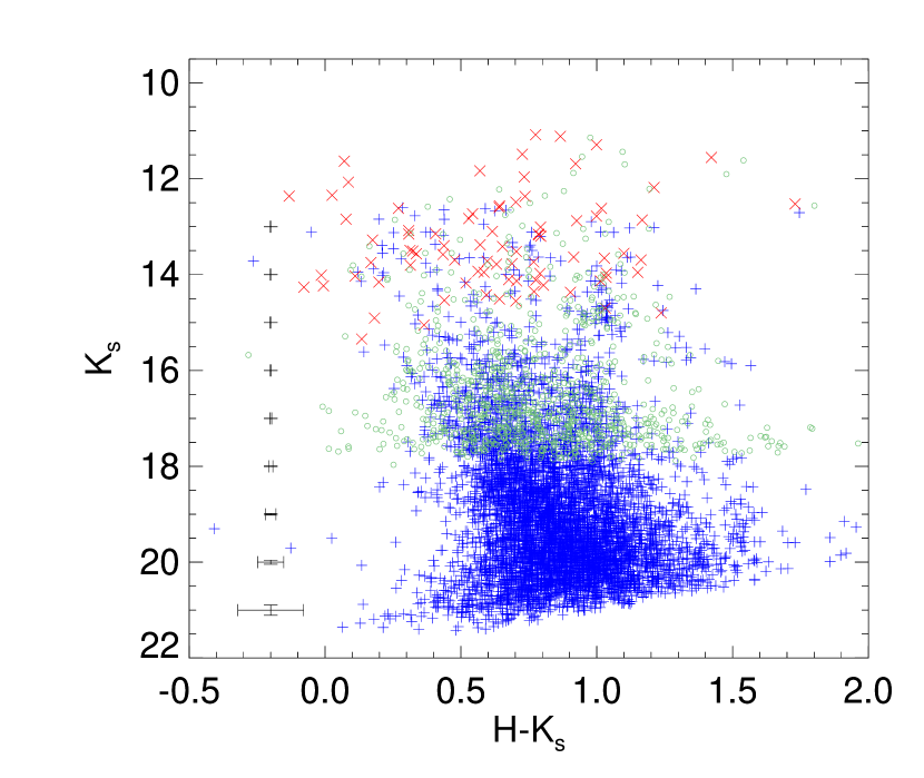
Figure 6: Colour–magnitude diagram with data from 2MASS, VVV and GSAOI in the $85\times 85$ arcsec² FoV of GSAOI. Uncertainties are indicated by error bars on the left. The symbols are the same as in Fig. 5.

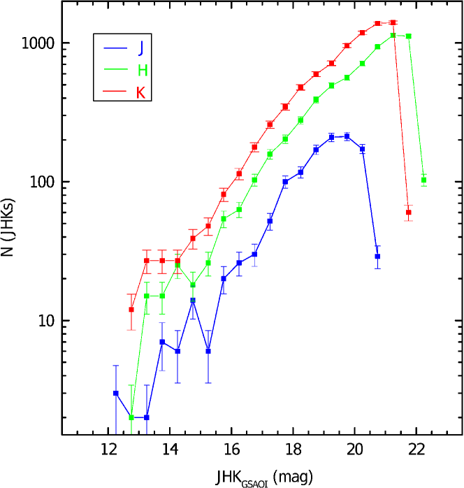
Figure 7: Number of stars detected as a function of magnitude for each near–infrared band.

3 Cluster centre and stellar density map

The equatorial coordinates of the candidate cluster were catalogued by Barbá et al. (2015) as $\alpha_{\rm J2000}=13^{\rm h}37^{\rm m}35.02^{\rm s}$ and $\delta_{\rm J2000}=-62\degr 40\arcmin 36.8\arcsec$, with Galactic coordinates $l=308\aas@@fstack{\circ}199$ and $b=-0\aas@@fstack{\circ}278$. The object centre coordinates were redetermined with the GSAOI data. The photometry was filtered to enhance the contrast between cluster and field stars: data in the range $K_{s}<18$ and $H-K_{s}>0.8$ yields the stellar density map shown in Fig. 8a. Such cutoffs select most of the cluster stars (see Sect. 4.2). On the other hand, data in the range $K_{s}<18$ and $H-K_{s}<0.8$ emphasizes the density map for field stars in Fig. 8b. As can be seen in Fig. 8, the cluster core presents an elongation nearly along the equatorial N-S direction, roughly aligned with Galactic N-S.

The centre determination relies on an algorithm that averages the stars’ coordinates within a circle of radius 12 arcsec, approximately the object core radius (see Sect. 6). This centre realocates the circle and a new centre is calculated yelding a new shift of the circle. The process is repeated until the difference between consecutive centres are smaller than a previously set quantity. To obtain a more physically meaningfull quantity, the density–weigthed centre was calculated using the same algorithm, but considering the stellar density at each star position as weight. The final equatorial coordinates derived from the procedure described above are: $\alpha_{\rm J2000}=13^{\rm h}37^{\rm m}35.4^{\rm s}$ and $\delta_{\rm J2000}=-62\degr 40\arcmin 34.7\arcsec$.

Figure 8: Stellar density map of LS 94 and field in the GSAOI FoV. (a) map limited in colour ($H-K_{\rm s}>0.8$) and magnitude ($K_{\rm s}<18$) to enhance the cluster contrast against the field. The centre (cross) and the adopted radius to search for this centre (circle) are indicated. (b) map complementary to that in (a), i.e., data selected for $H-K_{\rm s}<0.8$ and $K_{\rm s}<18$, to exclude cluster stars.

The cluster calculated centre and core radius are indicated by a cross and a circle, respectively, in Fig. 8. Note the object asymmetry revealing a disturbed stellar distribution and/or variable extinction. Since the Galactic longitude at this position runs almost parallel to the right ascension, may be we are witnessing the disruption of the cluster as a consequence of its interaction with the Galactic disc tidal field. But also its appearance could be partially explained as an artefact of differential reddening produced by filamentar interestelar clouds in front of the system. Spitzer images revealing the dust distribution in the region, on the contrary, do not show any particular feature which could possibly obscure stars preferentially in any direction around the cluster location. The relatively small FoV of GSAOI ($85\times 85$ arcsec²), is compensated by its excelent spatial resolution, which makes evident the cluster possible distorted morphology. This point is further discussed in Sect. 5.

4 Analysis of the stellar population

4.1 Radial variations

The analysis of the stellar content in annular regions of same area (Fig. 9) is presented in Figs. 10 and 11, which show photometric diagrams evidencing the progressive changes in the number of stars in different evolutionary stages from the cluster centre to the periphery. The photometry was filtered to show stars with $H-K_{\rm s}>0.8$ and $K_{\rm s}<18$. The inner circular field has radius 10 arcsec and the three subsequent external annuli, of same area as the inner circle, are bounded by 14, 17 and 20 arcsec.

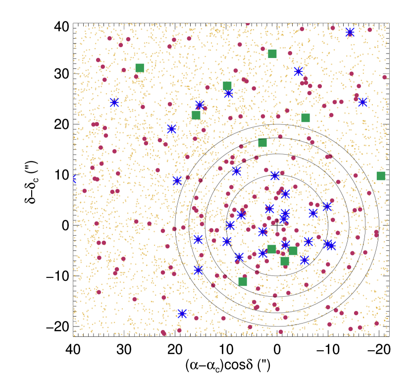
Figure 9: Spatial stellar distribution in the cluster region. Different symbols identify clump giant stars (RCG, blue asterisks), giant branch stars (green squares), main sequence stars (MS, red dots), field stars (small yellow dots). The black circles centred in the cluster delimit regions of identical area.

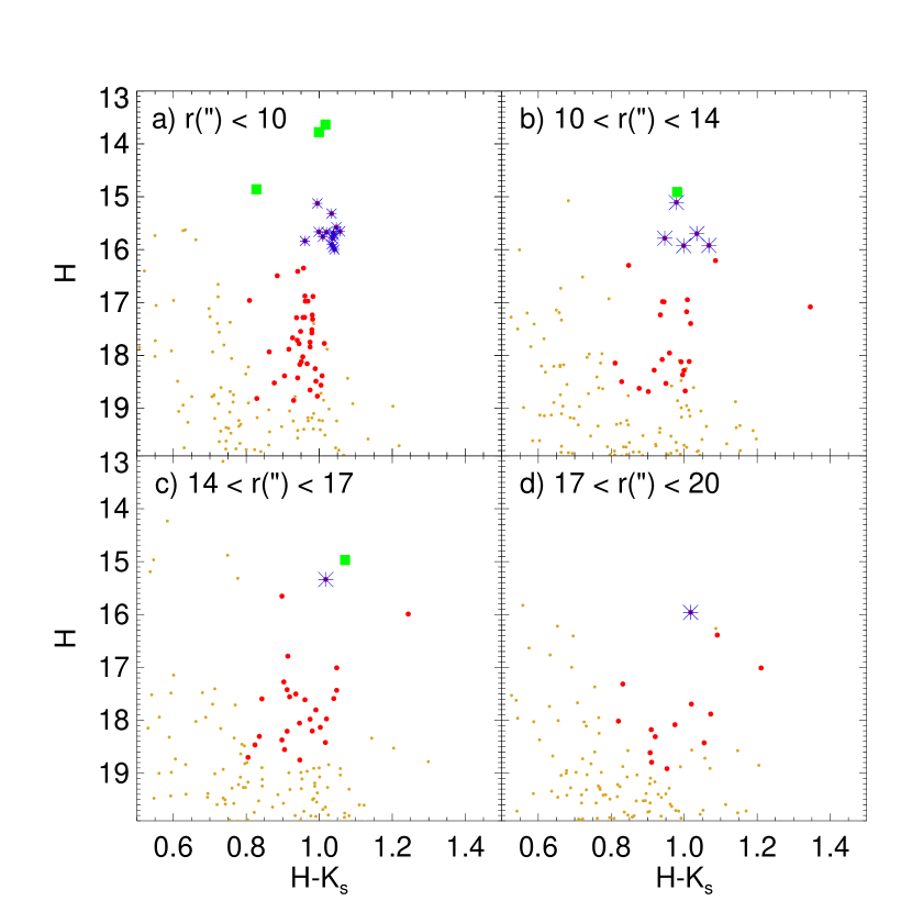
Figure 10: CMD $H$ vs $H-K_{\rm s}$ for each annular region shown in Fig. 9. The red dots are limited in colour ($H-K_{\rm s}>0.8$) and magnitude ($K_{\rm s}<18$). Symbols as in Fig. 9.

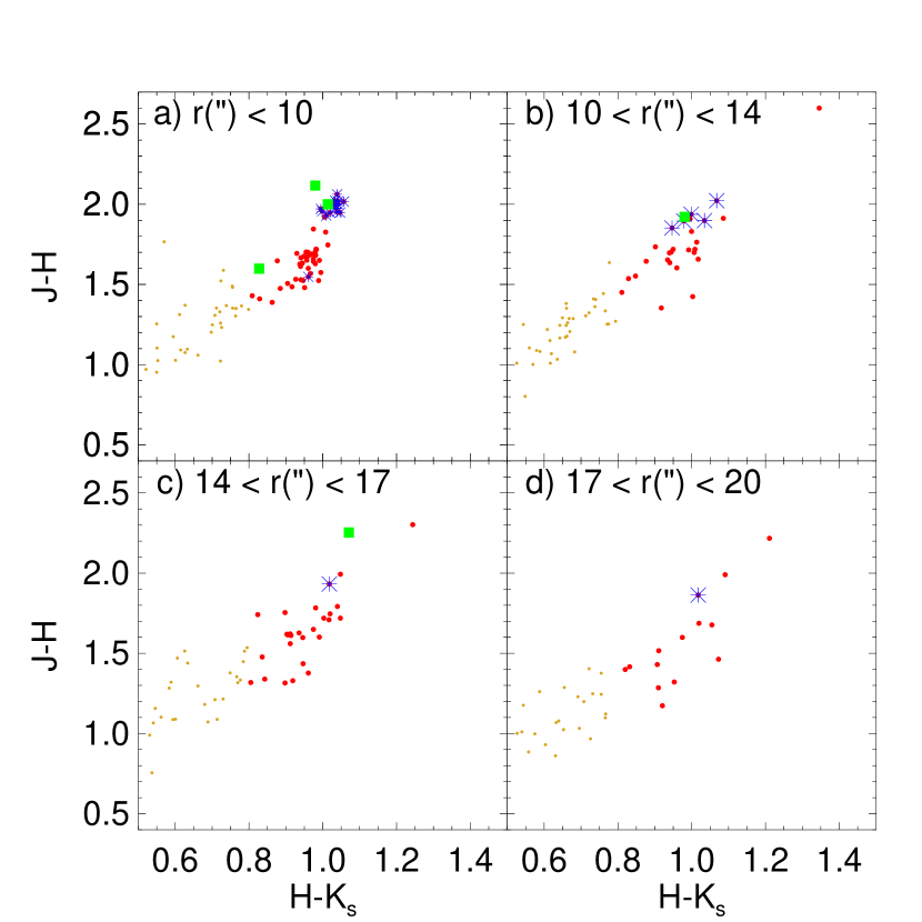
Figure 11: Same as Fig. 10 but for $J-H$ vs $H-K_{\rm s}$.

There is a tendency of red clump giant (RCG) stars to group by the cluster very centre, with most of them confined within 14 arcsec. The same is true for the red giants, but there are few of them, therefore this tendency can not be assured. Although main sequence (MS) stars are also concentrated within $r<10$ arcsec, there are many of them throughout the region up to 20 arcsec. To a deeper analysis of the stellar population it is necessary to disentangle the cluster members from the stars in the general Galactic disc field, which is done in the next Section.

4.2 CMD decontamination method and photometric membership

To disentangle cluster member stars from the contaminating stellar field it was employed a method that has been developed, tested and applied to Galactic open clusters. It recovers statistically the cluster intrinsic stellar population assigning membership probabilities to each star (Maia, Corradi & Santos Jr. 2010).

4.2.1 The method

The decontamination method deals with stellar photometry of the cluster and adjacent fields, both of same area. A CMD is built for both field and cluster plus field and divided in retangular cells of sizes corresponding roughly to ten times the average uncertainties in magnitude and colour. Because the GSAOI data is deeper for $H$ and $K_{\rm s}$ than for $J$, the former magnitudes were used in the decontamination procedure. After the initial setup, the number of stars is counted for the cluster region ($N_{clu+field}$) and for the control field ($N_{field}$) for every corresponding cell in both CMDs. A preliminary decontaminated sample is generated by removing the expected number of field stars from the cluster+field cells, prioritising the exclusion of the stars farther away from the cluster centre. An initial membership probability was assigned to all stars in the cluster region (even those removed from the CMD) according to their overdensity in each CMD cell relative to that in the field, i.e., $P=(N_{clu+field}-N_{field})/N_{clu+field}$. For cells containing more field stars than cluster stars, a zero probability was adopted.

To minimize the sensitivity of the method to the choice of initial parameters, the procedure is repeated for different sizes and positions of the cells. Their sizes are compressed and expanded by one third from the initial value (in both mag and colour) and their positions are shifted also by one third of the initial amounts towards negative and positive values. In total, 729 grid configurations are employed and the decontamination procedure described above is performed for each of them. An exclusion index is then defined as the number of times in which a given star is removed from the CMD. The final decontaminated sample is built by removing stars from the CMD with exclusion index above a predefined threshold. Similarly, the final photometric membership probability is obtained from the average of the membership probabilities assigned to each star.

Both the membership probability and the exclusion index actuate as complementary indicators since field stars can be identified for their low membership probability as well as for their high exclusion index. Tests of the method applied to photometry of Galactic open clusters and simulations of simple stellar populations indicated that a succesful decontamination is obtained when the exclusion index is around 80% (stars that are excluded in more than 80% of the 729 grid configurations are removed from the CMD) and the sample retains stars with membership probability above 30%. These thresholds were adopted for LS 94. The initial sizes of magnitude and colour cells were ($\Delta\,(H-K_{\rm s})$, $\Delta\,H$)=(0.2, 0.5). See Maia, Corradi & Santos Jr. (2010) for more details on the decontamination method.

4.2.2 Application

Two control fields (same area as the circular cluster region) were employed to compare the results of decontaminating the central region of the cluster ($r<14$ arcsec): (i)  the region defined by a ring surrounding the cluster from $15<r<20$ arcsec and (ii)  the region displaced from the cluster centre by 36 arcsec along the same Galactic latitude, towards East mostly. Fig. 12a depicts these regions together with the cluster region for stars with $H-K_{\rm s}>0.8$ and $K_{\rm s}<18$, just to enhance the contrast between cluster and field stars. Figs. 13 and 14 show the decontaminated CMDs using each control field, without any colour or magnitude filtering. The grid represents one cell configuration and the vertical colourbar reflects the membership probability assigned to each star. It is clear that the annular field contains MS stars below the turnoff belonging to the cluster. The decontamination method eliminates most stars with $H>18.5$. On the other hand, when the circular control field towards East is considered, the low MS is retained by the decontamination method. Therefore, a better account of cluster members was pursued in which a larger circular area was considered to include those MS stars. To do this, the decontamination method was applied to fields of $r<20$ arcsec, shown in Fig. 12b. As for the previous analysis, the control field was displaced from LS 94 centre towards East, and at the same Galactic latitude. The result is presented in Fig. 15.

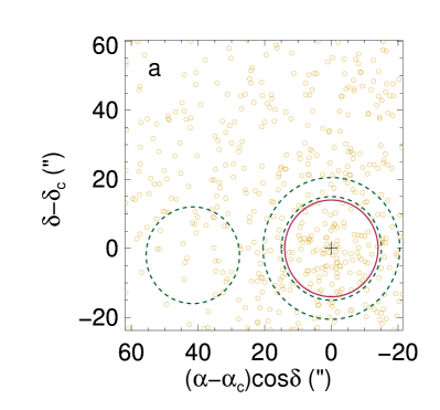
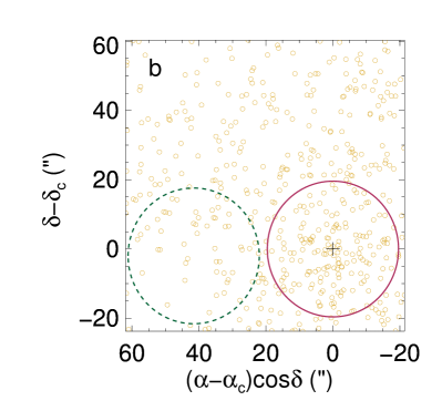
Figure 12: (a) The positions of the two stellar fields (dashed lines) used to decontaminate the CMD of the cluster region (continuous line). All regions have the same area. The star positions (yellow circles) are indicated for stars with $H-K_{\rm s}>0.8$ and $K_{\rm s}<18$, for contrast purposes. (b) Same as panel (a), but for a larger field and cluster areas.

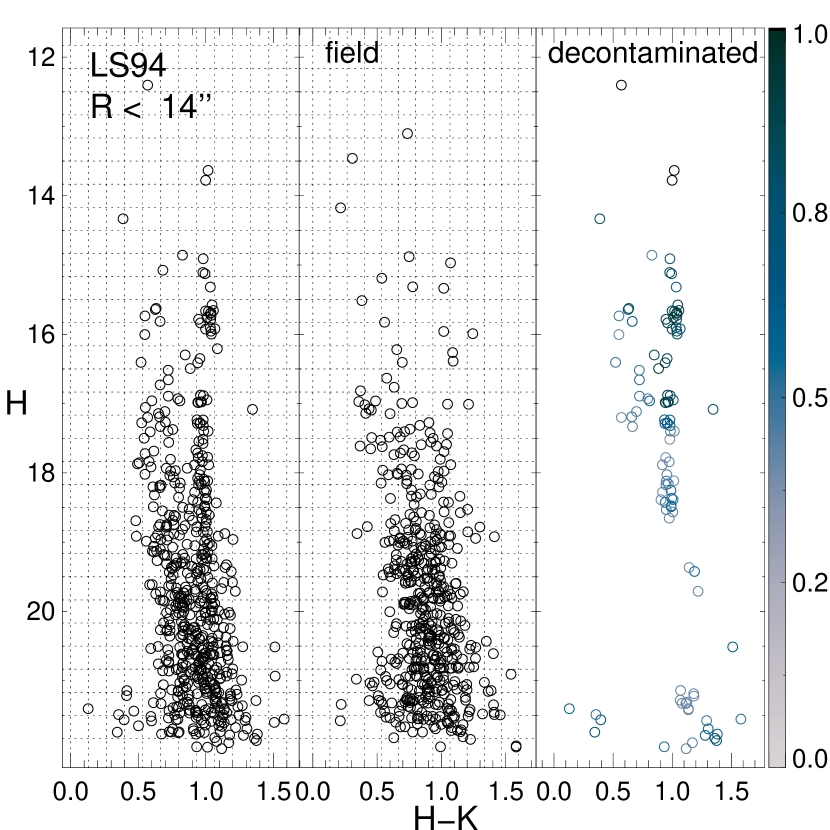
Figure 13: Decontamination of LS 94 CMD using as control field the annular area surrounding the cluster. Left: the CMD for the spatial region of the cluster defined by $R<14$ arcsec. Middle: the CMD of a neighbouring field covering the same area as the cluster region. The grid shows one of the 729 configurations of cell positions and size employed by the decontamination method. Right: The CMD of the decontaminated sample with stellar membership probabilities indicated by the colourbar.

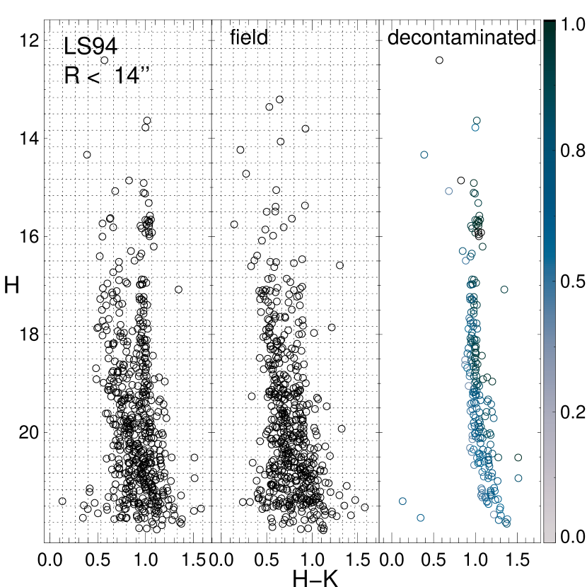
Figure 14: Same as Fig. 13 but using as control field the circular area adjacent to the cluster.

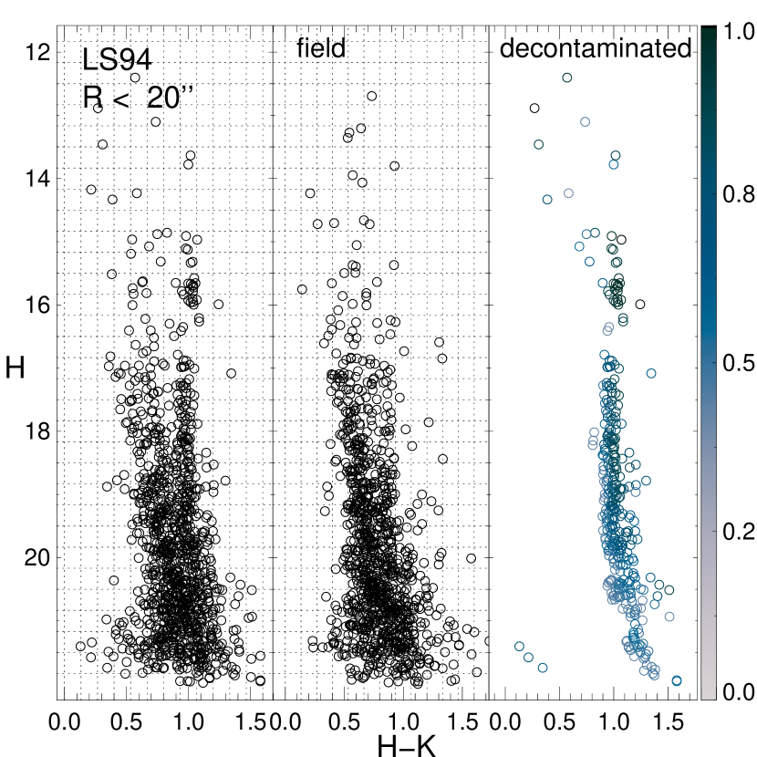
Figure 15: Decontamination of LS 94 CMD using the circular area with $r<20$ arcsec for both cluster and surrounding field. Symbols as in Fig. 13.

It is worth noticing that additional control fields were tested toward other directions about 40 arcsec from the cluster centre, with similar results as the one obtained for the circular field. Since the circular control field located as in Fig.12b has its centre at the same Galactic latitude as the cluster centre, it was assumed to give the best representation of the field over the cluster area, minimising the disc stellar population gradient and, possibly, differential reddening. Indeed, the similar colour width of the stellar populations observed in both cluster and field CMDs of Fig. 15 makes us confident that the subjacent stellar population and the reddening are not very different for them.

5 Fundamental parameters

5.1 Reddening

The reddening was inferred from the decontaminated colour–colour diagram (TCD) $J-H$ vs $H-K_{\rm s}$ and the intrinsic 2MASS near–infrared colours for dwarfs and giants covering a broad range of temperatures (Strayzis & Lazauskaite 2009). Specifically, the intrinsic colours of the RCG, where stars burn helium in their cores, were compared to the colours measured for the observed RCG. The RCG intrinsic averaged colors, ($J-H$)${}_{\circ}=0.46\pm 0.02$ and ($H-K_{\rm s}$)${}_{\circ}=0.09\pm 0.03$, are based on more than a hundred stars in six well–studied open clusters, and correspond to spectral type G8 III (Strayzis & Lazauskaite 2009). The average for the 19 RCG stars within 14 arcsec of LS 94 yields $\langle J-H\rangle=1.94\pm 0.11$ and $\langle H-K_{\rm s}\rangle=1.02\pm 0.03$, which are values reddened, consequently, by E($J-H$)$=1.48\pm 0.11$ and E($H-K_{\rm s}$)$=0.93\pm 0.04$. Using the Rieke & Lebofsky (1985) extintion law, the following quantities were derived: $E(B-V)=4.59\pm 0.23$, $A_{V}=14.18\pm 0.71$, $A_{K_{\rm s}}=1.59\pm 0.08$.

Fig. 16 is the TCD containing the stars considered members of LS 94, the intrinsic sequences of dwarfs and giants and the positions of the intrinsic RCG and of the LS 94 reddened RCG. These positions are linked by a straight line representing the reddening towards the cluster inner core, where the RCG stars are located. The locus of the best–fitting isochrone of age $\log{t}=9.12$ and metallicity $Z=0.019$ (see Sect. 5.4) is also shown there.

The position of the cluster turnoff is about $\langle H\rangle=16.90\pm 0.02$, $\langle H-K_{\rm s}\rangle=1.00\pm 0.02$, $\langle J-H\rangle=1.70\pm 0.03$. Using these colors as starting point in the TCD, a new line was drawn keeping the same slope and extent as determined by the reddening calculated from the RCG. The line end point lies on the expected location of intrinsic colours of dwarfs, which suggests that RCG giants and MS stars, with different spatial distributions over the cluster region, are affected by nearly the same reddening. This analysis links the intrinsic colours of the cluster turnoff with spectral type F8–G0 V.

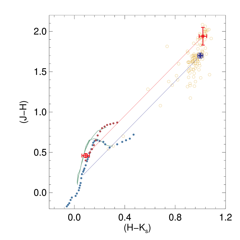
Figure 16: Colour–colour diagram of LS 94 members (yellow circles). Intrinsic colors of giants (red dots) and MS stars (blue dots) from Strayzis & Lazauskaite (2009). The red straight line connects intrinsic and LS 94 reddened positions of the RCG (red symbols with error bars). The blue straight line connects intrinsic and LS 94 reddened locus of the turnoff (blue symbol with error bars). The green continuous line is the locus of an isochrone with $\log{t}=9.12$ and $Z=0.019$.

The spatial distribution of the extinction was also investigated by constructing an extinction map based on the complete sample of stars within 20 arcsec from the cluster centre. To this end, an extinction value was calculated for each star by dereddening it along the reddening vector in the TCD, up to the MS locus defined by the $\log t$=9.12 ($Z=0.019$) isochrone. However, since only a small fraction of the sample possesses $J$ band magnitudes, we have repeated this procedure using the larger sample provided by the stars’ $H-K_{\rm s}$ colour only and the isochrone mean intrinsic colour ($H-K_{\rm s}$)_∘=0.0827. Because the first extinction estimate was based on $JHK_{s}$ photometry benefiting from a broad range of possible intrinsic colours, it was used to calibrate the less reliable values obtained from employing exclusively $H$-$K_{s}$ colours, revealing that this latter approach overestimate extinction by 1.0 mag on average (for details on the method, see Maia, Moraux & Joncour 2015). These calibrated extinction values were interpolated into an uniform grid with a resolution of 0.5 arcsec, the modal star separation in the field, and finally smoothed by a 1.5 arcsec width median kernel to build the final map shown in Fig. 17. The map reveals a complex pattern, dominated by a heavier extinction strip in the N-S direction, nearly perpendicular to the Galactic disc, presenting values between $13<A_{V}<16$. However, most of the region shows lower extinction values. To derive the cluster’s fundamental parameters we used the extinction derived from the position of the RCG stars, as they are clear members located in the cluster central region.

Confronting extinction (Fig. 17) and stellar density (Fig. 8) maps allowed us to infer that the elongated shape formed by the stellar distribution inside the cluster core cannot be produced by an artefact of enhanced extinction around its E-W borders, since the central parts of the cluster have higher extinction than its surroundings. Notwithstanding the existence of differential extinction in the region, the previous argument rules out the dust as responsible for the disturbed appearance of the cluster core.

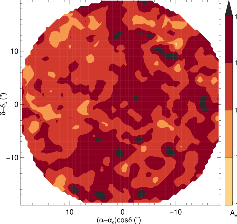
Figure 17: Extinction map derived for the inner 20 arcsec of LS 94.

5.2 Distance

The cluster distance was determined from the absolute magnitude of the RCG stars. Their absolute magnitude is an efficient distance indicator of a stellar system, especially in the near–infrared bands, where the uncertainties in the population age and metallicity are negligible compared to optical bands (Alves 2000; Grocholski & Sarajedini 2002).

Van Helshoecht & Groenewegen (2007), using 2MASS data for 24 open clusters with known distances, obtain $M_{K_{\rm s}}$(RCG)$=-1.57\pm 0.05$, arguing that this value is reliable for distance determinations of clusters with metallicities between $-0.5$ and $+0.4$ dex and ages between approximately 300 Myr and 8 Gyr. Assuming this absolute magnitude and the value measured for the apparent magnitude of the cluster RCG, i.e., $\langle K_{\rm s}\rangle$(RCG)$=K=14.67\pm 0.24$, the true distance modulus was calculated adopting the extinction $A_{K_{\rm s}}=1.59\pm 0.08$. The result is ($m-M$)${}_{\circ}=14.65\pm 0.26$, which leads to a distance of $d=8.5\pm 1.0$ kpc for LS 94.

5.3 Location in the Milky Way

The IAU–recommended value for the distance to the Galactic centre, $R_{\circ}=8.5$ kpc, has been revised by several authors using different methods. A recent compilation (from studies between 1990 and 2012) aimed at estimating $R_{\circ}$, enabled Gillessen et al. (2013) to indicate as the most probable value $R_{\circ}=8.20\pm 0.35$ kpc. This value was adopted to calculate the cluster Galactocentric distance from its distance to the Sun derived above. The result, $R=7.30\pm 0.49$ kpc, places the cluster $\sim 1$ kpc inside the solar circle.

Fig. 18 depicts the MW plane with the main spiral arms according to the representation by Portegies-Zwart, McMillan & Gieles (2010), which is based on Valée (2008). The Galactic centre, the bar and the sun position are indicated, as well as the solar orbit (solar circle) and the position of LS 94. The cluster lies in the Crux arm, in the fourth quadrant, inside the solar circle.

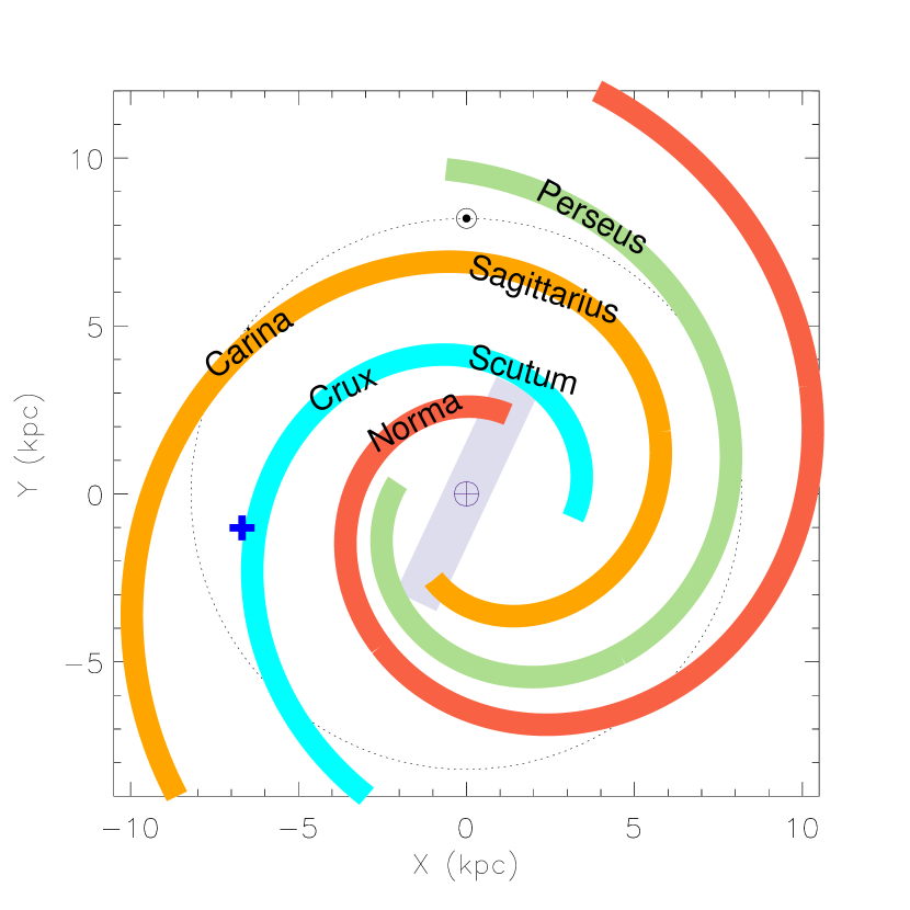
Figure 18: Representation of the MW plane with known spiral arms marked. The sun position and its orbit (dotted line) are shown together with the the Galactic centre (crossed circle), the bar and the position of LS 94 (blue cross).

5.4 Age and metallicity

To derive age and metallicity, PARSEC isochrones version 1.2S (Bressan et al. 2012; Chen et al. 2015) were fit to cluster CMDs decontaminated from field stars. Reddening and distance modulus as derived in Sect. 5 were applied to the data before the isochone fitting.

Fig. 19 shows the best–fitting isochrones to the intrinsic CMDs $M_{K_{\rm s}}$ vs ($J-K_{\rm s}$)_∘ and $M_{H}$ vs ($H-K_{\rm s}$)_∘. The region of RCG stars is zoomed to give a better sense of isochrone age and metallicity differences and how they match the data.

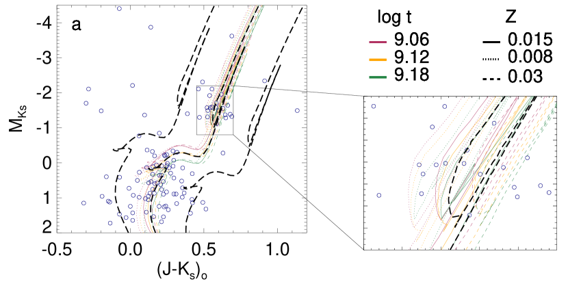
Figure 19: Isochrone match to the CMDs $M_{K_{\rm s}}$ vs ($J-K_{\rm s}$)_∘ (panel a) and $M_{H}$ vs ($H-K_{\rm s}$)_∘ (panel b). A set of isochrones covering ages $\log{t}=9.06,9.12,9.18$ and metallicities $Z=0.008,0.015,0.03$ is superimposed over the cluster CMDs. The best–fitting isochrone with $\log{t}=9.12$ and $Z=0.02$ is shown besided by the same isochrone shifted according to 2 $\sigma$ uncertainties in extinction and distance (black long–dashed lines). The RCG region is zoomed to make clearer the isochrone differences and their match to the data.

Although the CMD composed of $J$ and $K_{s}$ bands is shallower than that involving $H$ and $K_{s}$ bands, the former provides a longer baseline, allowing a more precise determination of age and metallicity. Also, to perform the reasonable isochrone fitting seen on the $M_{H}$ vs ($H-K_{\rm s}$)_∘ CMD, the extinction coefficient $A_{H}$ needed to be increased from 0.175 $A_{V}$ to 0.178 $A_{V}$, a value in agreement with extinction laws by Cardelli, Clayton & Mathis (1989) and Indebetouw et al. (2005). In conclusion, taking into account the range of isochrones that fit the cluster intrinsic CMDs, the age and metallicity determined for LS 94 are $\log{t}=9.12\pm 0.06$ and $Z=0.02\pm 0.01$.

The effect of the uncertainties in the distance modulus and extinction is also presented in Fig. 19, where the best–fitting isochrone with the age and metallicity determined above is shown together with the same isochrone displaced by amounts given by the uncertainties (2 $\sigma$) in E($H-K_{\rm s}$) (0.04), E($J-K_{\rm s}$) (0.12), $A_{K}$ (0.08), $A_{H}$ (0.12) and ($m-M$)_∘ (0.26). The data plotted cover the whole set of stars which survived the decontamination method, although outliers that are clearly non–members due to their positions in the CMDs, were retained in Fig. 19.

6 Cluster structure

6.1 Radial density profile

The cluster structure was investigated by building its radial density profile (RDP) using annuli of several widths to evaluate stellar densities from star counting. The annuli are centred in the derived cluster position (Sect.  3). Despite the cluster distortions evidenced by the density map (Sect. 3), the RDP shows a clear overdensity that falls significantly until 20 arcsec, nearly at the border of the frame (Fig. 20).

The star counts were performed for data filtered in $K_{\rm s}$ ($<18$) and $H-K_{\rm s}$ ($>0.8$) to enhance cluster to field contrast. However, it is worth noticing that these limits also mean that the RDP does not count lower MS stars with $M_{K_{\rm s}}>1.76$ or masses below 1.56 M_⊙ according to the derived distance, reddening and age (see Sect. 5). Coupled with the small GSAOI FoV, the already mentioned extended population of lower MS stars, would make a determination of the cluster tidal radius through the fitting of a three–parameter King (1962) model not useful. An estimate of the cluster core radius is given in the next section, but a discussion on its tidal radius is postponed to Sect. 7, where the cluster mass is derived.

Figure 20: LS 94 radial density profile. Different bin sizes are indicated by different symbols.

6.2 Central surface density and core radius

To estimate the central surface density and the core radius of LS 94, the CMD decontaminated sample (for $r<20$ arcsec) up to the completness limit ($H<21.2$) was subjected to a two–parameter King (1962) model fitting (Fig. 21). Because the selected data sample was already decontaminated, the stellar density background is null. The fitting (Fig. 21) provides $\sigma_{\circ}=(0.48\pm 0.04)$ stars/arcsec² for the cluster central stellar density and $r_{\rm c}=(12.3\pm 1.0)$ arcsec for its core radius. With the distance derived in Sect. 5, the scale is 1 arcsec=0.0412 pc and the converted values are $\sigma_{\circ}=283\pm 24$ stars/pc² and $r_{\rm c}=0.51\pm 0.04$ pc, respectively.

Figure 21: LS 94 RDP and the two–parameter King model fitting (dashed line) with envelope of 1 $\sigma$ uncertainties (dotted lines). Symbols as in Fig. 20. The fitting residuals are also presented in the lower panel.

Although the King model fitting was successful and useful to estimate $\sigma_{\circ}$ and $r_{\rm c}$, the cluster RDP has wiggles and bumps, compatible with a system in an advanced stage of evolution. Particularly, the central density is marginally described by the model. Taken directly from the observed RDP, the inner data point corresponds to $\sigma_{\circ}=0.64\pm 0.23$ stars/arcsec² or $38\pm 14\times 10$ stars/pc². The RDP central cusp is a known characteristic of evolved stellar systems like globular clusters with colapsed cores (Trager, King & Djorgovski 1995) and old open clusters (Momany et al. 2008; Bonatto et al. 2010).

Given the small FoV of GSAOI, a tidal radius was not fit, but obtained from the estimated total cluster mass, which was calculated by adding the observed stellar mass and that extrapolated to lower MS stars according to a mass function (see Sect. 7.2).

6.3 Mass segregation

Using the same decontaminated data as above, the two–parameter King model fitting was performed for different $H$ magnitude cutoffs, i.e., in addition to the completeness limit $H=21.2$, the cutoff was progressively decreased from 20.5 to 16, with intervals of 0.5 mag. Recalling that the turnoff is around $H=16.9$, if the cutoff is at $H=17$ then only evolved stars will be included in the fitting. The results are presented in Fig. 22, where the $r_{\rm c}$ obtained from the profile fitting is plotted as a function of the magnitude cutoff.

Figure 22: The core radius variation as a function of the magnitude cutoff. Stars brighter than the cutoff were included in the King model fitting to derive the core radius.

The cluster core radius increases whenever the magnitude cutoff includes more MS stars. It appears to be a transition around $H\sim 18.7$ where brighter stars are centrally concentrated ($r_{\rm c}\sim 0.38$ pc) while fainter stars are less concentrated ($r_{\rm c}\sim 0.55$ pc). Assuming that the overall core radius up to the completeness limit (Fig. 21) is a fiducial cluster core radius ($r_{\rm c}\sim 0.51\pm 0.04$ pc), then it indicates that the mass segregation occurs essentially inside the cluster core.

Beyond the population gradient shown in Fig. 10, the structural parameters gave additional information about the cluster dynamical state. In the next Section, a quantitave analysis of the stellar population distribution is given, also corroborating with these results.

7 Cluster integrated properties and tidal radius

7.1 Mass

The cluster mass inside its core ($r_{\rm c}<12$ arcsec) was derived from the observed $M_{H}$ luminosity function (LF) converted to a mass function (MF) with the aid of the best–fitting isochrone mass–luminosity relation. The LF for the core region is compared with that of an external region ($r_{\rm c}<r<20$ arcsec) in Fig. 23. The LFs include all stars from the decontaminated sample. The outer region LF contains more stars because its area is larger than that of the inner region and it may also be affected more significantly by differential extinction. The range of stellar masses sampled by the LF ($-3.5<M_{H}<4.7$) is $2.13>m$(M_⊙)$>0.71$ with the turnoff ($M_{H}=-0.27$) mass at $\sim$1.96 M_⊙. To model the stellar mass distribution where it is unseen or incomplete, a power–law MF was employed, namely $A=m^{-(1+x)}$, where $A$ is a normalization constant and $x$ the slope.

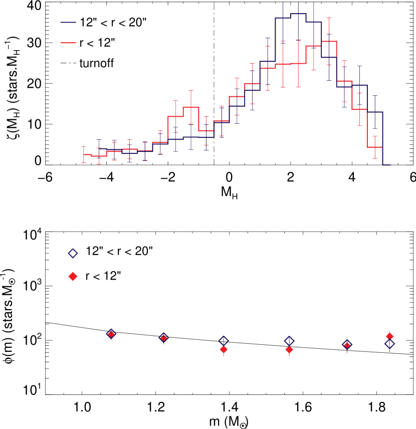
Figure 23: The luminosity function (top) and the mass function (bottom) of LS 94 from the decontaminated sample for two regions centred in the cluster. The fitting to the mass function yielded 0.7 for its slope and is represented by the continuous line. The uncertainties indicated by error bars come from Poisson statistics applied to the star counts.

Although the completeness limit for the whole FoV in the $H$ band (21.2) reaches $M_{H}=4.02$ or $m=0.88$ M_⊙, the MF normalization was chosen at the LF peak ($M_{H}\sim 3.5$ and $m=1.01$ M_⊙), which is a better constraint for the cluster (more crowded) region. Considering the core region, the total mass for stars more massive than 1.01 M_⊙ was estimated in $220\pm 21$ M_⊙. Between $1.01$ and $1.89$ M_⊙, the distribution of MS stars was fit by the power–law giving $x=0.7$ for its slope (Fig. 23), which served to extrapolate the MF down to 0.5 M_⊙. From there to the H–burning mass limit (0.08 M_⊙) it was assumed that the slope flattens to $x=0.3$, in accord with a Kroupa (2001) MF. Integration of the MF yields the partial masses $91\pm 6$ M_⊙ between $1.01$ and $0.5$ M_⊙ and $130\pm 57$ M_⊙ between 0.5 and 0.08 M_⊙. Therefore, the total mass in the core is the sum of the three quoted values, i.e., $441\pm 61$ M_⊙.

Bonatto & Bica (2005) analysed a sample of open clusters of different ages and concluded that there is a strong correlation between the core mass and the overall mass, regardless of how populous is the cluster (see their fig. 9d). From our estimate for the core mass and their results, it leads to the overall cluster mass of $6\pm 1$ times bigger than that of the core, that is $\mathcal{M}=(2.65\pm 0.57)\times 10^{3}$ M_⊙. The number of stars associated with this mass is $\approx$3600.

7.2 Tidal radius

The cluster tidal radius is poorly constrained by the small region sampled by GSAOI but it can be estimated using the cluster total mass and the MW rotation curve parameters. According to Xin & Zheng (2013, and references therein), the MW rotation curve circular velocity at the Galactocentric distance of LS 94 ($R=7.30\pm 0.49$ kpc) is $V_{\rm c}=250\pm 30$ km/s. Consequently, the Galaxy mass inside the cluster orbit results $\mathcal{M}_{g}=1.00\pm 0.07\times 10^{11}$ M_⊙.

The tidal radius of an open cluster with disc kinematics (King 1962) can be estimated by

$$r_{\rm t}=\left(\frac{G\mathcal{M}}{4\mathcal{A}(\mathcal{A}-\mathcal{B})}\right)^{1/3}$$ (4)

where $\mathcal{A}=14.82\pm 0.84$ km s^-1 kpc^-1 and $\mathcal{B}=-12.37\pm 0.64$ km s^-1 kpc^-1 (Feast & Whitelock 1997) are the Oort (1927) constants. Inserting into this equation the cluster mass $\mathcal{M}$ leads to $r_{\rm t}=19.2\pm 1.4$ pc.

Another estimate for LS 94 tidal radius may be obtained from the expression (King 1962):

$$r_{\rm t}=R\left(\frac{\mathcal{M}}{3\mathcal{M}_{g}}\right)^{1/3}$$ (5)

In this case, $r_{\rm t}=15.1\pm 1.5$ pc was obtained. Both equations 4 and 5 are equivalent but give independent tidal radius estimates since they rely on different sets of observational parameters. Averaging both values provides our final estimate: $r_{\rm t}=17.2\pm 2.1$ pc. Combining the derived cluster radii $r_{\rm t}$ and $r_{\rm c}$, the concentration parameter ($c=\log{r_{t}/r_{c}}$) follows, $c=1.53\pm 0.06$. All these structural parameters estimates should be taken as approximations considering that LS 94, as already pointed out, is dynamically evolved undergoing mass segregation and the models were designed to describe massive symmetric systems in dynamic equilibrium.

The relaxation time ($t_{r}$) of a stellar system with $N$ stars can be defined as $t_{r}=\frac{N}{8\ln{N}}t_{cr}$, where $t_{cr}=r/\sigma_{V}$ is the time–scale for a star to cross a distance $r$ with velocity $\sigma_{V}$ (Binney & Tremaine 1987). The time–scale in which the cluster tends to kinetic energy equipartition, transfering massive stars to its core and low mass stars to its corona is what $t_{r}$ measures. To calculate $t_{r}$ for LS 94, a typical value of $\sigma_{V}\approx 3$ km/s found for open clusters (Binney & Merrifield 1998) was used together with $r_{\rm t}$ and $r_{\rm c}$ obtained above and also the respective number of stars $N_{t}\approx 3600$ inside $r_{\rm t}$ and $N_{c}\approx 600$ inside $r_{\rm c}$. The result is $t_{r}\approx 5.5$ Myr for the cluster core and $t_{r}\approx 300$ Myr for the whole cluster. Compared to the cluster age, 1.3 Gyr, the much shorter $t_{r}$ indicates that the cluster had time to reach an advanced stage of relaxation (faster in the core) compatible with the mass segregation observed.

7.3 Luminosity

The $J$, $H$ and $K_{\rm s}$ integrated absolute magnitudes were calculated by adding up the brightness of selected member stars in the CMD. The selected subsample of members was chosen according to a colour filter based on the best–fitting isochrone. Members that are farther from the isochrone than 3 $\sigma$ of the uncertainty in extinction are excluded from the calculation of integrated light. The subsample was defined independently for three CMDs of each magnitude as ordinate, e.g., the $J$ band was combined with every possible colour $J-H$, $J-K_{\rm s}$ and $H-K_{\rm s}$. Fig. 24 shows the nine combinations of magnitudes and colours with red symbols identifying the selected stars used to compute the integrated magnitudes and green crosses marking the best–fitting isochrone ($\log{t}=9.12$ and $Z=0.02$) locus.

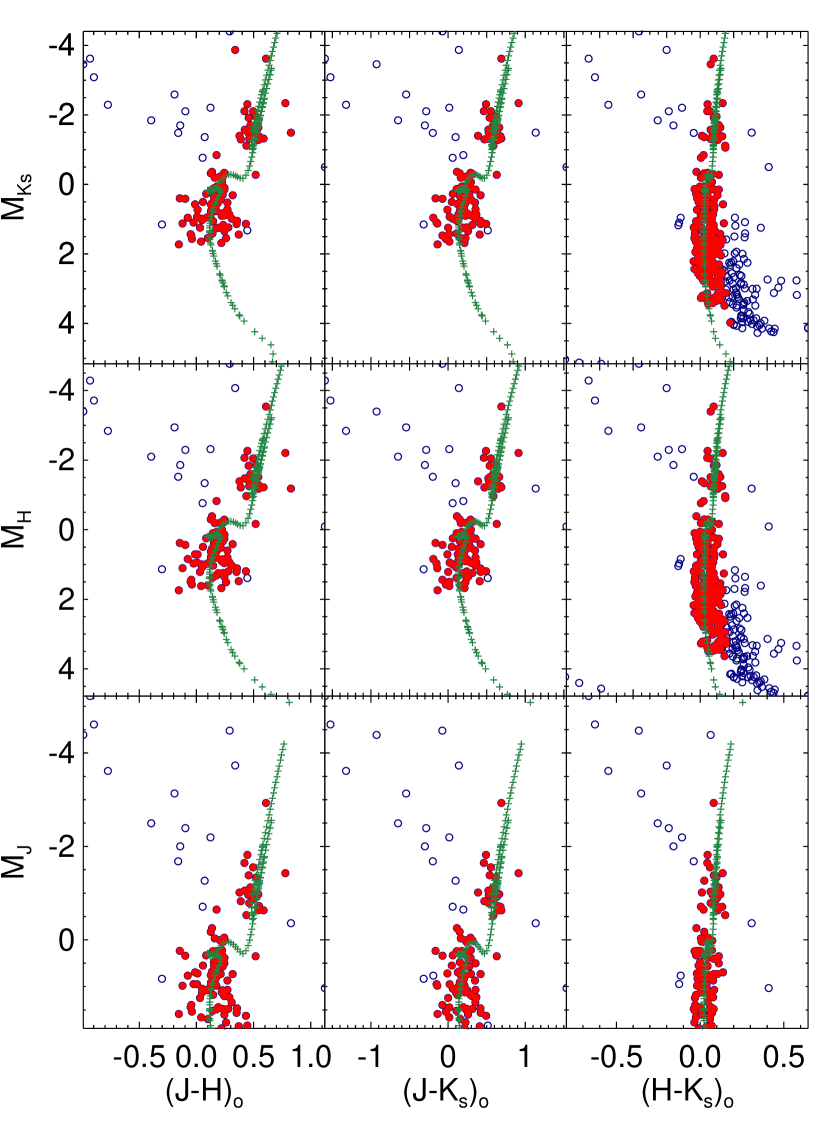
Figure 24: Decontaminated CMDs with all possible combinations of magnitudes and colours. Red filled circles indicate the subsample of stars that lie not farther from the best–fitting isochrone than 3 $\sigma$ of the uncertainties in extinction. Blue open circles represent stars excluded from the calculation of the integrated magnitude. The locus of the best–fitting isochrone is marked by green crosses.

Therefore, for each row of Fig. 24 there are three values of integrated magnitude obtained for the same band, which rely on independent datasets. Whenever the J band is involved, the CMD reaches a shallower magnitude limit. To account for the low MS in all CMDs, the observed LF was extrapolated from the completeness limit according to the MF used to determine the cluster mass. The sum of the flux of individual stars added to the flux extrapolated using the MF gives the integrated magnitude. There are two important points to raise in this context: (i) the integrated magnitudes are dominated by bright stars, which are subject to stochastic effects that in turn induce fluctuations in the integrated light (Cerviño 2013, and references therein), especially in the near–infrared for intermediate–age to old clusters, which means that clusters with significantly different integrated magnitudes may underlie stellar populations with similar age and metallicity (Santos Jr. & Frogel 1997); (ii) the decontamination method does not perform efficiently in CMD regions where the number of stars is small, as is in the present case for bright stars, i.e., discriminating between bright field and member stars is hampered by the small number statistics. This is why a colour filter helps to better constrain the cluster population. Keeping these points in mind, the final integrated magnitudes are $M_{J}=-5.30\pm 0.06$, $M_{H}=-5.70\pm 0.17$ and $M_{K_{\rm s}}=-5.82\pm 0.16$. These are, indeed, lower limits for the cluster integrated light since they were estimated for stars within $r<20$ arcsec $=0.82$ pc, about 1.6 times the cluster core radius. However, bright member stars are not expected to be found beyond the cluster core given its advanced stage of evolution.

To check the consistency between the integrated magnitudes and mass estimates, simple stellar population models were built from the $\log{t}=9.12$ and $Z=0.019$ isochrone with stars distributed as prescribed by the same MF employed above. The estimated integrated magnitudes were interpolated in the models to get the mass, resulting $3.29\pm 0.77\times 10^{3}$ M_⊙, which is in agreement, within the uncertainties, with the total mass estimated for the cluster.

8 Discussion

The final parameters adopted for LS 94 are summarized in Table 2.

The differential reddening across the cluster area cannot reproduce the observed elongated stellar distribution of the cluster core, as argued in Sec. 5. Therefore, the distortions showing up in the surface density map reveal a stellar system disturbed by gravitational interactions with the Galactic disc material. With 1.3 Gyr and located inside the solar circle, at $R=7.3$ kpc from the Galactic centre, the cluster should have completed many orbits, loosing stars to the Galactic field by a combination of internal stellar and dynamical evolution with external processes like disc shocking, molecular cloud encounters and gravitational stresses from spiral arms (Spitzer 1987; Gieles et al. 2006). All these external mechanisms impart cumulative tidal effects to the cluster after many passages on its way throughout the disc. The elongated shape of LS 94 core, with semimayor axis oriented perpendicular to the Galactic disc is expected if the main mechanism actuating in the present time on the cluster is disc shocking (Bergond, Leon & Guibert 2001; Dalessandro et al. 2015). To clarify this issue, further investigation of the cluster kinematics would be needed.

The RDP presents a cusp in the very centre, characteristic of evolved clusters. Indeed, mass segregation in the cluster core seems to be occurring, with most of the RCG stars (14) concentrating within $r<0.4$ pc (10 arcsec) and MS stars distributing themselves more evenly by the cluster core and outskirts. This behaviour is also detected as an increase of the core radius with the magnitude level cutoff defining the star sample. Stars more massive than $m\sim 1.65$ M_⊙ ($H=18.7$) are spatially distributed accordingly to a King model with $r_{\rm c}\sim 0.38$ pc, while stars less massive than this value are better represented by $r_{\rm c}\sim 0.55$ pc. In addition, the slope of the cluster MF $x=0.7$ is flatter than that of the Kroupa (2001) MF for masses higher than 0.5 M_⊙, also suggesting mass segregation.

Carraro et al. (2014) report 12 clusters older than 1 Gyr and closer to the Galactic centre than the solar circle. Although there are many more clusters within this selection criterion, they were chosen for their well–determined ages and distances. In this context, LS 94 parameters fits among those of this sample, including the higher than solar metallicity (recalling that $Z=0.015$ is the sun metallicity for PARSEC isochrones).

Concerning structural parameters, LS 94 is not as loose as those investigated by Bonatto & Bica (2005), which studied eleven open clusters spanning broad age and mass ranges. The six clusters with ages above 1 Gyr (three of them inside the solar circle) have concentration parameter around $c\sim 1.0$, lower than that calculated for LS 94 ($c\sim 1.5$). Comparing with Galactic globular clusters (Harris 1996, (2010 edition)), the LS 94 concentration parameter is within the average: 26 per cent of the globulars out of 141 with structure information have $c=1.5\pm 0.2$.

Table 2: Parameters determined for LS 94.

$E(B-V)$	$4.59\pm 0.23$
$A_{V}$	$14.18\pm 0.71$
$A_{K_{\rm s}}$	$1.59\pm 0.08$
$(m-M)_{\circ}$	$14.65\pm 0.26$
$d$ (kpc)	$8.5\pm 1.0$
$age$ (Gyr)	$1.3\pm 0.2$
$Z$	$0.02\pm 0.01$
$R$ (kpc)	$7.30\pm 0.49$
$\sigma_{\circ}$ (10 stars/pc2)	$38\pm 14$
$r_{\rm c}$ (pc)	$0.51\pm 0.04$
$r_{\rm t}$ (pc)	$17.2\pm 2.1$
$c$	$1.53\pm 0.06$
$t_{\rm r}$ core (Myr)	$\approx 5.5$
$t_{\rm r}$ overall (Myr)	$\approx 300$
$\mathcal{M}$ ($10^{3}$ M⊙)	$2.65\pm 0.57$
$M_{K_{\rm s}}$	$-5.82\pm 0.16$

9 Summary and concluding remarks

Physical properties were derived for the candidate open cluster La Serena 94, recently unveiled by the VVV collaboration. The object’s position is in the Galactic midplane under the influence of severe extinction towards the Crux spiral arm. Deep photometry in $JHK_{\rm s}$–bands from GeMs/GSAOI was employed to characterize the object. The projected stellar density distribution of the region, conveyed into a 2D map, provided information on the location of the cluster centre and its overall structure. An analysis of the stellar population radial variation from the determined centre showed direct evidence of mass segregation with RCG stars centrally concentrated, while MS stars spread farther into the cluster outskirsts. Decontaminated $JHK_{\rm s}$ diagrams were built reaching stars with about 5 mag below the cluster turnoff in $H$. The locus of RCG stars in the TCD, together with an extinction law, was used to obtain an average extinction of $A_{V}=14.18\pm 0.71$. The same stars were considered as standard–candles to derive the cluster heliocentric distance, $d=8.5\pm 1.0$ kpc. Isochrones were matched to the member stars locii in CMDs to derive age ($\log{t}=9.12\pm 0.06$) and metallicity ($Z=0.02\pm 0.01$). The cluster structure was investigated further by fitting King models to its RDP, in spite of a central cusp and ragged appearance. An overall core radius of $r_{\rm c}=0.51\pm 0.04$ pc was obtained. King models fittings to magnitude limited star samples evidenced mass segregation as well, as the core radius shrinks from fainter to brigther stellar samples. The cluster core mass was derived by adding up the visible stellar mass to an extrapolated MF built from the LF in the $H$–band. A correction to this mass leads to $\mathcal{M}=(2.65\pm 0.57)\times 10^{3}$ M_⊙ for the cluster total mass. The $JHK_{\rm s}$ integrated magnitudes were computed by summing up the star fluxes, resulting $M_{J}=-5.30\pm 0.06$, $M_{H}=-5.70\pm 0.17$ and $M_{K_{\rm s}}=-5.82\pm 0.16$. Consistency between mass and magnitude estimates were checked by comparing them with those of synthetic stellar populations of same age and metallicity as those of the cluster. With the cluster mass determined, an estimate of the tidal radius was possible: $r_{\rm t}=17.2\pm 2.1$ pc.

The fundamental parameters of LS 94 confirm that it is an old open cluster located in the Crux spiral arm towards the fourth Galactic quadrant and distant $7.30\pm 0.49$ kpc from the Galactic centre. From our perspective, the cluster light propagates roughly 3 kpc through the Crux arm and another 5.5 kpc through the Galactic disc before reaching us. The cluster age and distorted structure already suggested that it is a dinamically evolved stellar system. Also, its position inside the solar circle is expected to speed up the cluster dynamical evolution in consequence of stronger tidal effects (Bergond, Leon & Guibert 2001; Bonatto & Bica 2005). Further analyses confirmed that, indeed, with an overall relaxation time 4 times shorter than its age and clear evidences of mass segregation, the cluster is at the final stages of evolution before the remnant phase when most of the stars are lost into the Galactic disc (Pavani et al. 2011, and references therein). This conclusion was also confirmed by the structural analysis of the cluster RDP, which showed a transition of the core radius for stars in different mass intervals, and the stellar mass distribution, which revealed a shallower MF slope compared with a Kroupa MF.

Continuing efforts to uncover distant clusters and derive their properties are needed to fill the gap which reveal our Galaxy structure, as open clusters are one of its tracers (Dias & Lépine 2005; Frinchaboy & Majewski 2008). In particular, observations of obscured, distant star clusters with 8–m class telescopes and sensitive near–infrared instruments incorporating AO, like GeMs/GSAOI, will contribute to increase the sample of well–studied clusters towards the third and fourth Galactic quadrants, where few systems have been characterized.

References

- Alves (2000) Alves D., 2000, ApJ, 539, 732
- Barbá et al. (2015) Barbá R. H., et al., 2015, preprint, (arXiv:1505.02764)
- Barbaro & Pigatto (1984) Barbaro G., Pigatto L., 1984, A&A, 136, 355
- Bergond, Leon & Guibert (2001) Bergond G., Leon S., Guibert J., 2001, A&A, 377, 462
- Binney & Merrifield (1998) Binney J., Merrifield M., 1998, Galactic Astronomy. Princeton Univ. Press, Princeton, NJ
- Binney & Tremaine (1987) Binney J., Tremaine S., 1987, Galactic Dynamics. Princeton Univ. Press, Princeton, NJ
- Bonatto & Bica (2005) Bonatto C., Bica E., 2005, A&A, 437, 483
- Bonatto et al. (2010) Bonatto C., Ortolani S., Barbuy B., Bica E., 2010, MNRAS, 402, 1685
- Borissova et al. (2014) Borissova J. et al., 2014, A&A, 569, 24
- Bressan et al. (2012) Bressan A., Marigo P., Girardi L.,Salasnich B., Dal Cero C., Rubele S., Nanni A., 2012, MNRAS, 427, 127
- Camargo, Bica & Bonatto (2015) Camargo D., Bica E., Bonatto C., 2015, NewA, 34, 84
- Cardelli, Clayton & Mathis (1989) Cardelli J. A., Clayton G. C., Mathis J. S., 1989, ApJ, 345, 245
- Carraro et al. (2014) Carraro G., Giorgi E. E., Costa E., Vázquez R. A., 2014, MNRAS, 441, 36
- Carraro, Ng & Portinari (1998) Carraro G., Ng Y. K., Portinari L., 1998, MNRAS, 296, 1045
- Carrasco et al. (2012) Carrasco E. R. et al., 2012, Proc. SPIE, 8447, 8447N
- Cerviño (2013) Cerviño M., 2013, New Astronomy Reviews, 57, 123
- Chen et al. (2015) Chen Y., Bressan A., Girardi L., Marigo P., Kong X., Lanza A., 2015, MNRAS, 452, 1068
- Dalessandro et al. (2015) Dalessandro E., Miocchi P., Carraro G., Jílková L., Moitinho A., 2015, MNRAS, 449, 1811
- De Silva, Freeman & Bland-Hawthorn (2009) De Silva G. M., Freeman K. C., Bland-Hawthorn J., 2009, PASA, 26, 11D
- Dias & Lépine (2005) Dias W. S., Lépine J. R. D., 2005, ApJ, 629, 825
- Diolaiti et al. (2000) Diolaiti E., Bendinelli O., Bonaccini D., Close L., Currie D., Parmeggiani G., 2000, A&AS, 147, 335
- Dutra & Bica (2001) Dutra C. M., Bica E. 2001, A&A, 376, 434
- Feast & Whitelock (1997) Feast M., Whitelock P., 1997, MNRAS, 291, 683
- Friel (1995) Friel E. D. 1995, ARA&A, 33, 381
- Frinchaboy & Majewski (2008) Frinchaboy P. M., Majewski S. R., 2008, AJ, 136, 118
- Gieles et al. (2006) Gieles M., Portegies Zwart S. F., Baumgardt H., Athanassoula E., Lamers H. J. G. L. M., Sipior M., Leenaarts J., 2006, MNRAS, 371, 793
- Gillessen et al. (2013) Gillessen S., Eisenhauer F., Fritz T. K., Pfuhl O., Ott T., Genzel R., 2013, in Advancing the Physics of Cosmic Distances, Proc. IAU Symp. 289, 29
- Grocholski & Sarajedini (2002) Grocholski A. J., Sarajedini A., 2002, AJ, 123, 1603
- Harris (1996) Harris W. E., 1996, AJ, 112, 1487
- Hou, Chang & Chen (2002) Hou J.-L., Chang R.-X., Chen L., 2002, Chin. J. Astron. Astrophys., 2, 17
- Indebetouw et al. (2005) Indebetouw R. et al., 2005, ApJ, 619, 931
- Ivanov et al. (2002) Ivanov V. D., Borissova J., Pessev P., Ivanov G. R., Kurtev R., 2002, A&A, 394, 1
- King (1962) King I., 1962, AJ, 67, 471
- Kronberger et al. (2006) Kronberger M. et al., 2006, A&A, 447, 921
- Kroupa (2001) Kroupa P., 2001, MNRAS, 322, 231
- Magrini et al. (2015) Magrini L. et al., 2015, A&A, 580, 85
- Maia, Corradi & Santos Jr. (2010) Maia F. F. S., Corradi W. J. B., Santos Jr. J. F. C., 2010, MNRAS, 407, 1875
- Maia, Moraux & Joncour (2015) Maia F. F. S., Moraux E., Joncour I., 2015, MNRAS, submitted
- McGregor et al. (2004) McGregor P. et al., 2004, Proc. SPIE, 5492, 1033
- Minniti et al. (2010) Minniti D. et al., 2010, New A, 15, 433
- Momany et al. (2008) Momany Y., Ortolani S., Bonatto C., Bica E., Barbuy B., 2008, MNRAS, 391, 1650
- Neichel et al. (2014a) Neichel B. et al., 2014a, MNRAS, 440, 1002
- Neichel et al. (2014b) Neichel B., Lu J. R., Rigaut F., Ammons S. M., Carrasco E. R., Lassalle E., 2014b, MNRAS, 445, 500
- Oort (1927) Oort J. H., 1927, Bull. Astron. Inst. Netherlands, 3, 275
- Pavani et al. (2011) Pavani D. B., Kerber L. O., Bica E., Maciel W. J., 2011, MNRAS, 412, 1611
- Piatti, Clariá & Abadi (1995) Piatti A. E., Clariá J. J., Abadi M. G., 1995, AJ, 110, 2813
- Portegies-Zwart, McMillan & Gieles (2010) Portegies Zwart S. F., McMillan S. L. W., Gieles M., 2010, ARAA, 48, 431
- Rieke & Lebofsky (1985) Rieke G. H., Lebofsky M. J., 1985, ApJ, 288, 618
- Rigaut et al. (2012) Rigaut F. et al., 2012, Proc. SPIE 8447, 84470I
- Rigaut et al. (2014) Rigaut F. et al., 2014, MNRAS, 437, 2361
- Saito et al. (2010) Saito R. et al., 2010, The Messenger, 141, 24
- Salaris, Weiss & Percival (2004) Salaris M., Weiss A., Percival S. M., 2004 A&A, 414, 163
- Santos Jr. & Frogel (1997) Santos Jr. J. F. C., Frogel J. A., 1997, ApJ, 479, 764
- Skrutskie (2006) Skrutskie M. F. et al., 2006, AJ, 131, 1163
- Spitzer (1987) Spitzer L., 1987, Dynamical Evolution of Globular Clusters. Princeton Univ. Press, Princeton, NJ
- Strayzis & Lazauskaite (2009) Strayzis V., Lazauskaite R., 2009, Baltic Astronomy, 18, 19
- Tody (1986) Tody D., 1986, The IRAF Data Reduction and Analysis System, in Proc. SPIE Instrumentation in Astronomy VI, ed. D. L. Crawford, 627, 733
- Trager, King & Djorgovski (1995) Trager S. C., King I. R., Djorgovski S., 1995, AJ, 109, 218
- Valée (2008) Valée J. P., 2008, AJ, 135, 1301
- van den Bergh (1996) van den Bergh S., 1996, PASP, 108, 986